
Behavioural Classification of Cattle Using Neck-Mounted Accelerometer-Equipped Collars

 ,
,  , , ,
, , ,  ,
,  ,
,  , , and
Abstract
:1. Introduction
2. Related Work
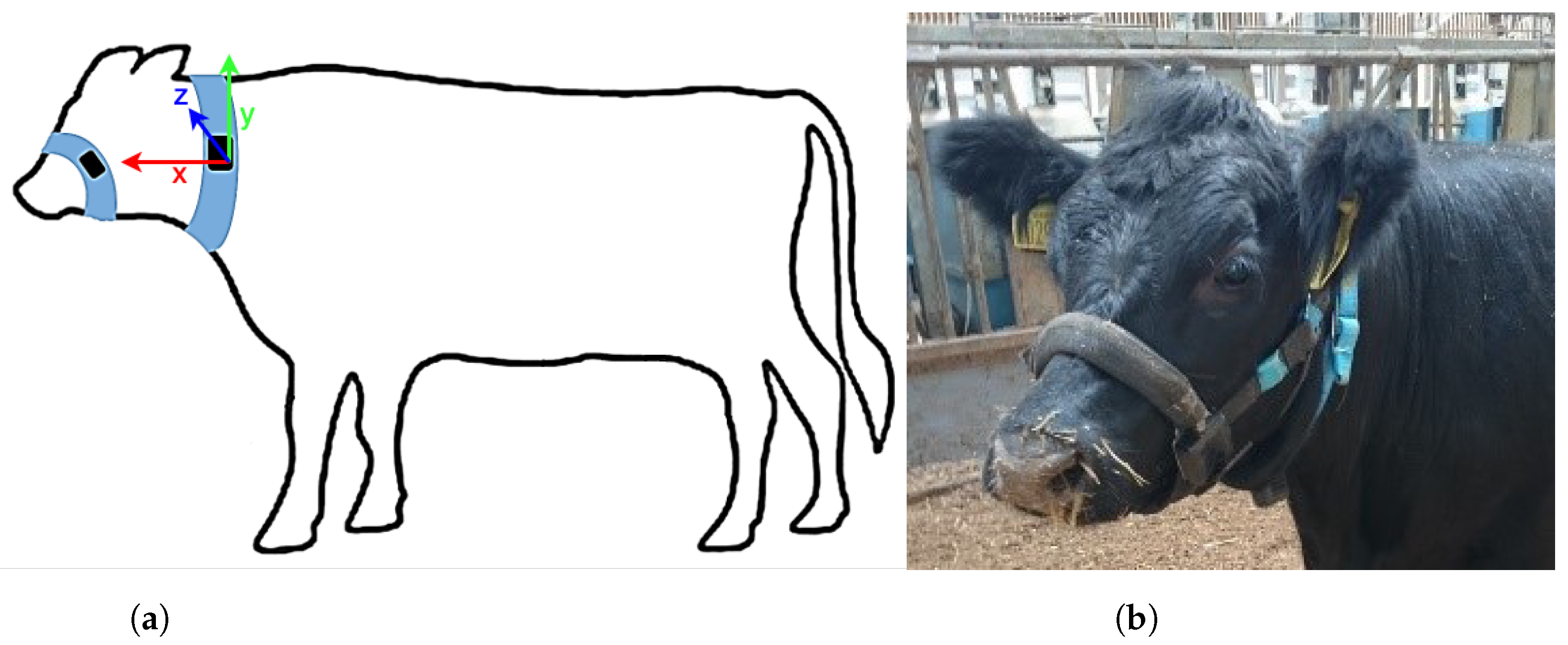
3. Data
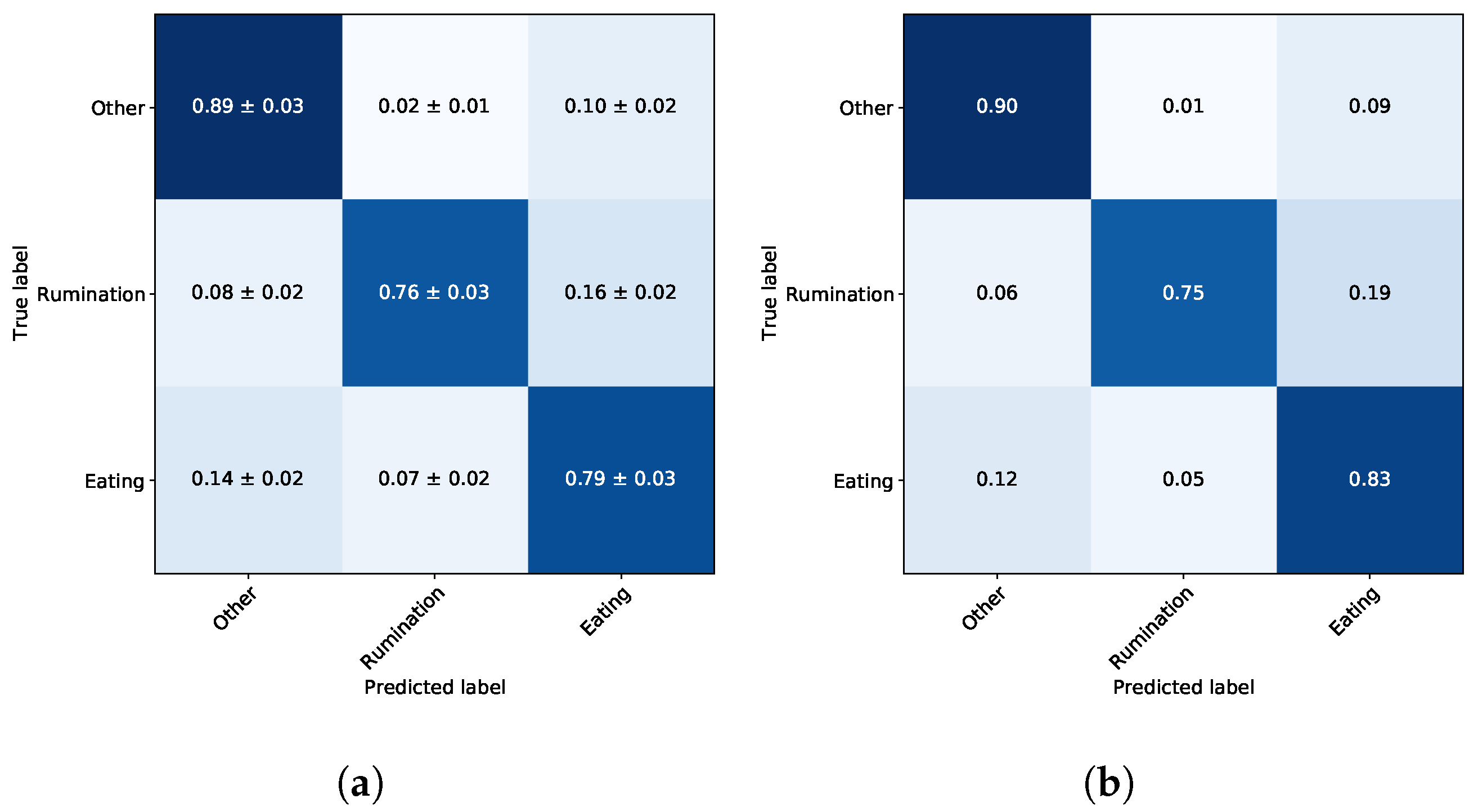
- Eating—the animal is ingesting food.
- Rumination—the animal is regurgitating to further breakdown ingested food and improve nutrient absorption.
- Other—the animal is engaged in an activity which is neither ruminating or eating.
Data Preparation
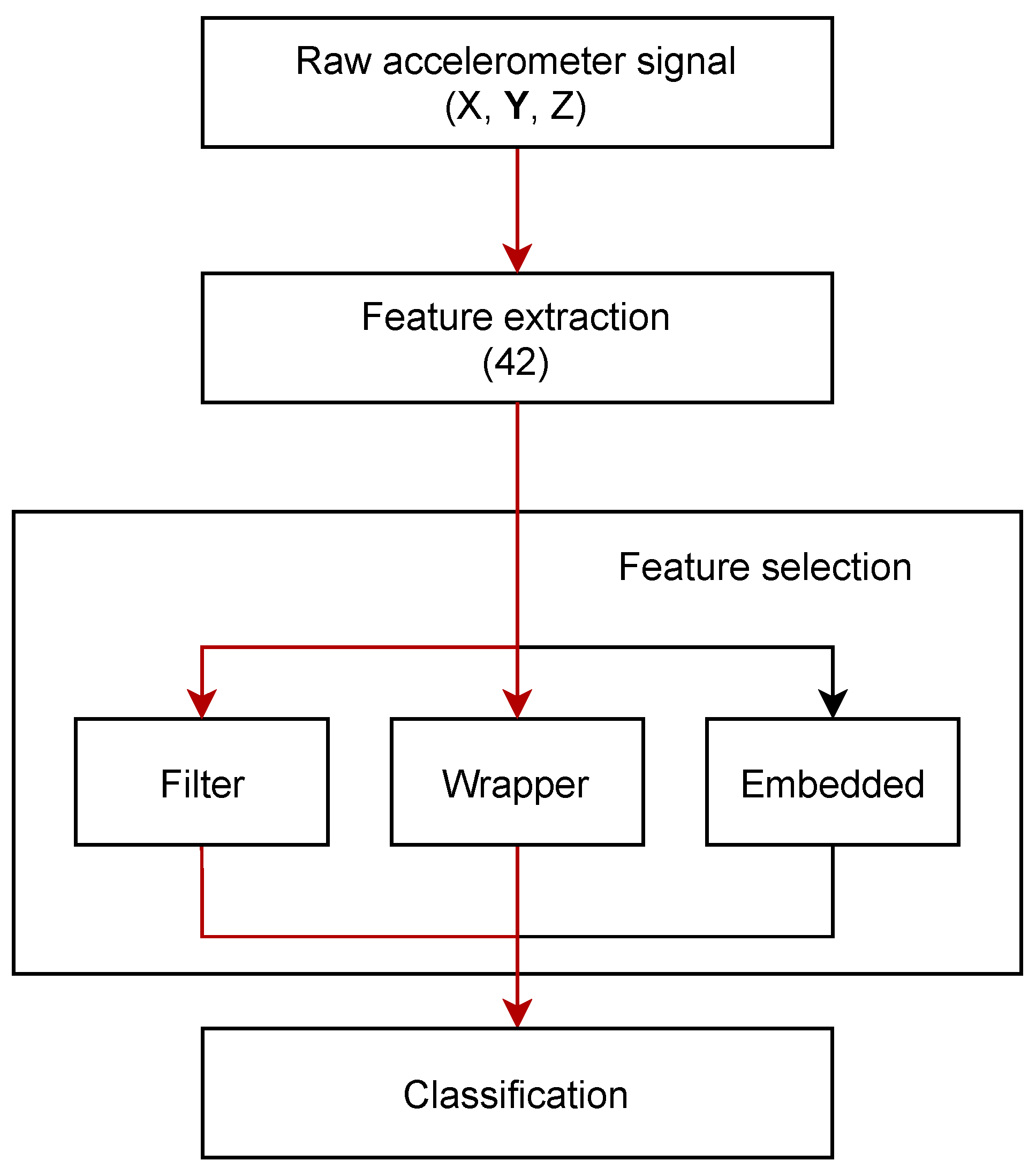
4. Model Design
4.1. Training and Validation
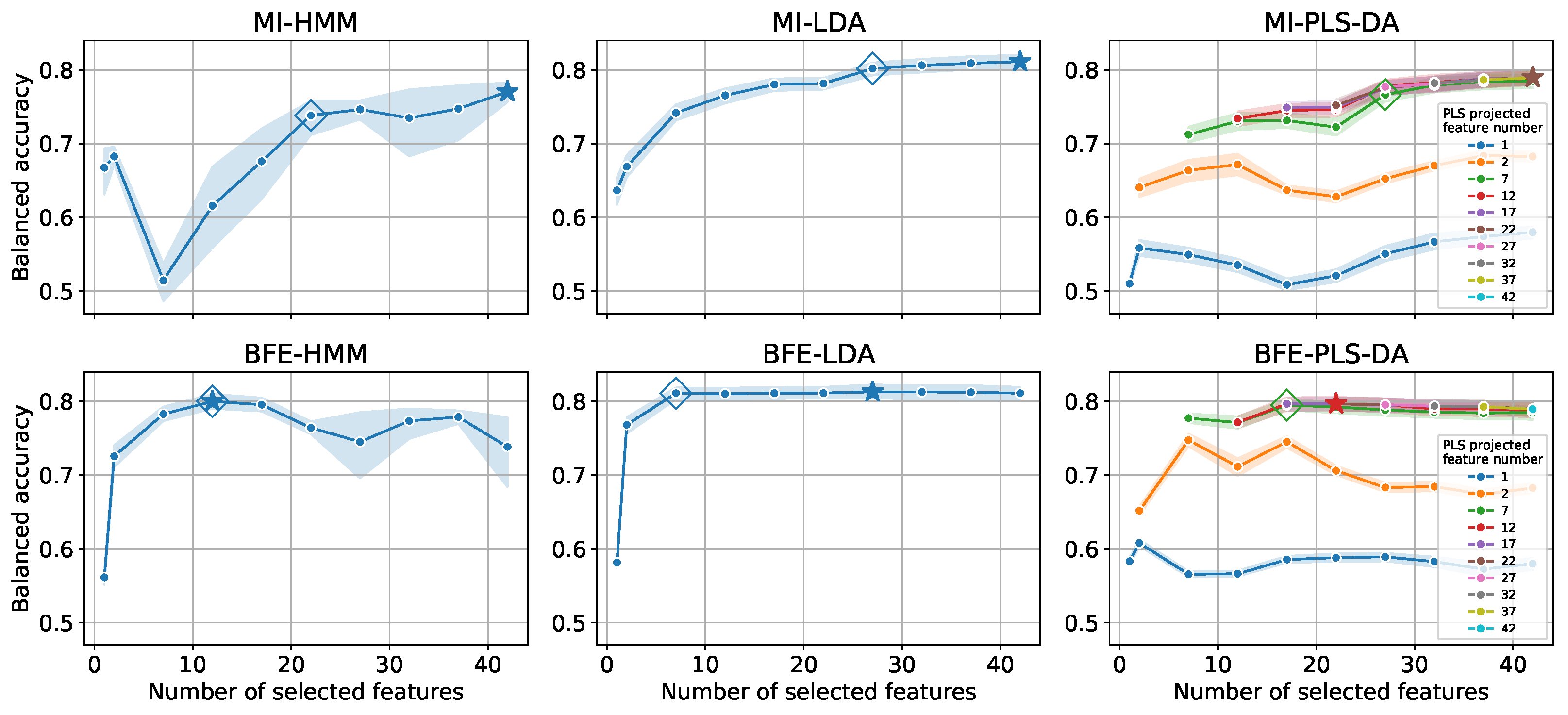
4.2. Feature Reduction
| Algorithm 1 Backward Feature Elimination procedure used to reduce features in blocks. | |
| ▹ Total features set | |
| ▹ Remaining features set | |
| P | ▹ Declare empty performance array |
| whiledo | |
| for 1 to R do | |
| ▹ Select subset of features | |
| model.fit | ▹ Train the model with |
| = model.eval | ▹ Compute model performance with features |
| end for | |
| where | ▹ Update remaining features by excluding low performing features |
| end while | |
5. Classification Algorithms
5.1. Hidden Markov Models
5.2. Linear Discriminant Analysis
5.3. Partial Least Squares Discriminant Analysis
6. Performance Evaluation
7. Conclusions
Author Contributions
Funding
Institutional Review Board Statement
Data Availability Statement
Acknowledgments
Conflicts of Interest
Appendix A

| Features | Definition |
|---|---|
| Aggregated autocorrelation | Standard deviation of autocorrelation function over a range of different values |
| Autoregressive coefficient | Coefficient of the unconditional maximum likelihood of an autoregressive process |
| Autocorrelation | |
| Benford correlation | Correlation of the time-series first digit distribution with N-B Law distribution |
| Binned entropy | |
| Change quantiles | Standard deviation of changes of the time-series within the first and third quartile range |
| Complexity-invariant distance | |
| Count above global mean | Number of observations higher than the mean value estimated on the training set |
| Count above local mean | Number of observations higher than the time-series mean |
| Count below global mean | Number of observations lower than the mean value estimated on the training set |
| Count below local mean | Number of observations lower than the time-series mean |
| c3 | |
| Energy | |
| FFT aggregated | Kurtosis of the absolute Fourier transform spectrum |
| FFT amplitude | Maximum of FFT magnitudes between 2 and 4 Hz |
| FFT coefficient | Sum of the FFT magnitudes between 2 and 4 Hz |
| First quartile | The value surpassed by exactly 25% of the time-series data points |
| Fourier entropy | Binned entropy of the time-series power spectral density |
| Kurtosis | Difference between the tails of analysed distribution and tails of a normal distribution |
| Lempel-Ziv complexity | Complexity estimate based on the Lempel-Ziv compression algorithm |
| Linear trend | Standard error of the estimated linear regression gradient |
| Longest strike above mean | Length of the longest sequence in time-series higher than its mean value |
| Longest strike below mean | Length of the longest sequence in time-series lower than its mean value |
| Maximum | The highest value in time-series |
| Median | The value surpassed by exactly 50% of the time-series data points |
| Minimum | The lowest value in time-series. |
| Number of CWT peaks | Number of peaks within ricker wavelet smoothed time-series |
| Number of peaks | Number of observations with a value higher than n neighbouring observations |
| Partial autocorrelation | |
| Permutation entropy | Entropy of ordering permutations occurring in fixed-length time-series window chunks |
| Range count | Number of observations between the first and the third time-series quartile |
| Ratio beyond r sigma | Percentage of observations diverging from the mean by more than r standard deviations |
| Sample entropy | Negative logarithm of the conditional probability that two sequences remain similar |
| Skewness | Distortion or asymmetry that deviates from the normal distribution |
| Spectral flatness | Ratio between geometric and arithmetic mean of the power spectrum |
| Spectral Welch density | Power spectral density estimation using the Welch method at a certain frequency |
| Standard deviation | |
| Sum of changes | |
| Third quartile | The value surpassed by exactly 75% of the time-series data points |
| Time-series sum | |
| Variation coefficient | Relative standard deviation, i.e., ratio of the standard deviation to the mean |
| Zero crossing | Number of points where time-series signal crosses a zero value |
References
- AHDB Dairy. AHDB Dairy Statistics. 2021. Available online: https://ahdb.org.uk/dairy (accessed on 17 February 2022).
- Fricke, P.M.; Carvalho, P.D.; Giordano, J.O.; Valenza, A.; Lopes, G.; Amundson, M.C. Expression and detection of estrus in dairy cows: The role of new technologies. Animal 2014, 8, 134–143. [Google Scholar] [CrossRef] [Green Version]
- Michie, C.; Andonovic, I.; Gilroy, M.; Ross, D.; Duthie, C.A.; Nicol, L. Oestrus Detection in Free Roaming Beef Cattle. In Proceedings of the European Conference on Precision Livestock Farming—EC-PLF 2013, Leuven, Belgium, 10–12 September 2013. [Google Scholar]
- Roelofs, J.B.; Van Erp-Van Der Kooij, E. Estrus detection tools and their applicability in cattle: Recent and perspectival situation. Anim. Reprod. 2015, 12, 498–504. [Google Scholar] [CrossRef]
- Afimilk/NMR. Silent Herdsman/Better Performing Cows; NMR: Chippenham, UK, 2012. [Google Scholar]
- Stangaferro, M.; Wijma, R.; Caixeta, L.; Al-Abri, M.; Giordano, J. Use of rumination and activity monitoring for the identification of dairy cows with health disorders: Part III. Metritis. J. Dairy Sci. 2016, 99, 7422–7433. [Google Scholar] [CrossRef] [Green Version]
- Rahman, A.; Smith, D.V.; Little, B.; Ingham, A.B.; Greenwood, P.L.; Bishop-Hurley, G.J. Cattle behaviour classification from collar, halter, and ear tag sensors. Inf. Process. Agric. 2018, 5, 124–133. [Google Scholar] [CrossRef]
- Zehner, N.; Niederhauser, J.J.; Nydegger, F.; Grothmann, A.; Keller, M.; Hoch, M.; Haeussermann, A.; Schick, M. Validation of a new health monitoring system (RumiWatch) for combined automatic measurement of rumination, feed intake, water intake and locomotion in dairy cows. In Proceedings of the Information Technology, Automation and Precision Farming. International Conference of Agricultural Engineering—CIGR-AgEng 2012: Agriculture and Engineering for a Healthier Life, Valencia, Spain, 8–12 July 2012. [Google Scholar]
- Poulopoulou, I.; Lambertz, C.; Gauly, M. Are automated sensors a reliable tool to estimate behavioural activities in grazing beef cattle? Appl. Anim. Behav. Sci. 2019, 216, 1–5. [Google Scholar] [CrossRef]
- Hamilton, A.W.; Davison, C.; Tachtatzis, C.; Andonovic, I.; Michie, C.; Ferguson, H.J.; Somerville, L.; Jonsson, N.N. Identification of the rumination in cattle using support vector machines with motion-sensitive bolus sensors. Sensors 2019, 19, 1165. [Google Scholar] [CrossRef] [Green Version]
- Martiskainen, P.; Järvinen, M.; Skön, J.P.; Tiirikainen, J.; Kolehmainen, M.; Mononen, J. Cow behaviour pattern recognition using a three-dimensional accelerometer and support vector machines. Appl. Anim. Behav. Sci. 2009, 119, 32–38. [Google Scholar] [CrossRef]
- Benaissa, S.; Tuyttens, F.A.; Plets, D.; Cattrysse, H.; Martens, L.; Vandaele, L.; Joseph, W.; Sonck, B. Classification of ingestive-related cow behaviours using RumiWatch halter and neck-mounted accelerometers. Appl. Anim. Behav. Sci. 2019, 211, 9–16. [Google Scholar] [CrossRef] [Green Version]
- Robert, B.; White, B.J.; Renter, D.G.; Larson, R.L. Evaluation of three-dimensional accelerometers to monitor and classify behavior patterns in cattle. Comput. Electron. Agric. 2009, 67, 80–84. [Google Scholar] [CrossRef]
- Abell, K.M.; Theurer, M.E.; Larson, R.L.; White, B.J.; Hardin, D.K.; Randle, R.F. Predicting bull behavior events in a multiple-sire pasture with video analysis, accelerometers, and classification algorithms. Comput. Electron. Agric. 2017, 136, 221–227. [Google Scholar] [CrossRef]
- González, L.A.; Bishop-Hurley, G.J.; Handcock, R.N.; Crossman, C. Behavioral classification of data from collars containing motion sensors in grazing cattle. Comput. Electron. Agric. 2015, 110, 91–102. [Google Scholar] [CrossRef]
- Riaboff, L.; Aubin, S.; Bedere, N.; Couvreur, S.; Madouasse, A.; Goumand, E.; Chauvin, A.; Plantier, G. Evaluation of pre-processing methods for the prediction of cattle behaviour from accelerometer data. Comput. Electron. Agric. 2019, 165, 104961. [Google Scholar] [CrossRef]
- Riaboff, L.; Poggi, S.; Madouasse, A.; Couvreur, S.; Aubin, S.; Bédère, N.; Goumand, E.; Chauvin, A.; Plantier, G. Development of a methodological framework for a robust prediction of the main behaviours of dairy cows using a combination of machine learning algorithms on accelerometer data. Comput. Electron. Agric. 2020, 169, 105179. [Google Scholar] [CrossRef]
- Kasfi, K.T.; Hellicar, A.; Rahman, A. Convolutional Neural Network for Time Series Cattle Behaviour Classification. In Proceedings of the Workshop on Time Series Analytics and Applications—TSAA’16, Hobart, TAS, Australia, 6 December 2016; ACM Press: New York, NY, USA, 2016; pp. 8–12. [Google Scholar] [CrossRef]
- Peng, Y.; Kondo, N.; Fujiura, T.; Suzuki, T.; Wulandari; Yoshioka, H.; Itoyama, E. Classification of multiple cattle behavior patterns using a recurrent neural network with long short-term memory and inertial measurement units. Comput. Electron. Agric. 2019, 157, 247–253. [Google Scholar] [CrossRef]
- Rahman, A.; Smith, D.; Hills, J.; Bishop-Hurley, G.; Henry, D.; Rawnsley, R. A comparison of autoencoder and statistical features for cattle behaviour classification. In Proceedings of the 2016 International Joint Conference on Neural Networks (IJCNN), Vancouver, BC, Canada, 24–29 July 2016; pp. 2954–2960. [Google Scholar] [CrossRef]
- Pavlovic, D.; Davison, C.; Hamilton, A.; Marko, O.; Atkinson, R.; Michie, C.; Crnojević, V.; Andonovic, I.; Bellekens, X.; Tachtatzis, C. Classification of Cattle Behaviours Using Neck-Mounted Accelerometer-Equipped Collars and Convolutional Neural Networks. Sensors 2021, 21, 4050. [Google Scholar] [CrossRef]
- ITIN+HOCH. RumiWatchSystem: Measurement System for Automatic Health Monitoring in Ruminants. 2014. Available online: https://www.rumiwatch.com/ (accessed on 17 February 2022).
- Christ, M.; Braun, N.; Neuffer, J.; Kempa-Liehr, A.W. Time Series FeatuRe Extraction on basis of Scalable Hypothesis tests (tsfresh—A Python package). Neurocomputing 2018, 307, 72–77. [Google Scholar] [CrossRef]
- Guyon, I.; Elisseeff, A. An introduction to variable and feature selection. J. Mach. Learn. Res. 2003, 3, 1157–1182. [Google Scholar]
- Fukunaga, K. Introduction to Statistical Pattern Recognition; Elsevier: Amsterdam, The Netherlands, 2013. [Google Scholar]
- Jović, A.; Brkić, K.; Bogunović, N. A review of feature selection methods with applications. In Proceedings of the 2015 38th International Convention on Information and Communication Technology, Electronics and Microelectronics (MIPRO), Opatija, Croatia, 25–29 May 2015; pp. 1200–1205. [Google Scholar]
- Saeys, Y.; Inza, I.; Larranaga, P. A review of feature selection techniques in bioinformatics. Bioinformatics 2007, 23, 2507–2517. [Google Scholar] [CrossRef] [Green Version]
- Kraskov, A.; Stögbauer, H.; Grassberger, P. Estimating mutual information. Phys. Rev. E 2004, 69, 066138. [Google Scholar] [CrossRef] [Green Version]
- Ross, B.C. Mutual information between discrete and continuous data sets. PLoS ONE 2014, 9, e87357. [Google Scholar] [CrossRef] [PubMed]
- Barber, D. Bayesian Reasoning and Machine Learning; Cambridge University Press: Cambridge, UK, 2012. [Google Scholar]
- Murphy, K.P. Machine Learning: A probabilistic Perspective; MIT Press: Cambridge, MA, USA, 2012. [Google Scholar]
- Bishop, C.M. Pattern Recognition and Machine Learning; Springer: Berlin/Heidelberg, Germany, 2006. [Google Scholar]
- Bilmes, J.A. A gentle tutorial of the EM algorithm and its application to parameter estimation for Gaussian mixture and hidden Markov models. Int. Comput. Sci. Inst. 1998, 4, 126. [Google Scholar]
- Tharwat, A.; Gaber, T.; Ibrahim, A.; Hassanien, A.E. Linear discriminant analysis: A detailed tutorial. AI Commun. 2017, 30, 169–190. [Google Scholar] [CrossRef] [Green Version]
- Martinez, A.M.; Kak, A.C. PCA versus LDA. IEEE Trans. Pattern Anal. Mach. Intell. 2001, 23, 228–233. [Google Scholar] [CrossRef] [Green Version]
- Lee, L.C.; Liong, C.Y.; Jemain, A.A. Partial least squares-discriminant analysis (PLS-DA) for classification of high-dimensional (HD) data: A review of contemporary practice strategies and knowledge gaps. Analyst 2018, 143, 3526–3539. [Google Scholar] [CrossRef] [PubMed]
- Haenlein, M.; Kaplan, A.M. A beginner’s guide to partial least squares analysis. Underst. Stat. 2004, 3, 283–297. [Google Scholar] [CrossRef]
- Brereton, R.G.; Lloyd, G.R. Partial least squares discriminant analysis: Taking the magic away. J. Chemom. 2014, 28, 213–225. [Google Scholar] [CrossRef]
- Pedregosa, F.; Varoquaux, G.; Gramfort, A.; Michel, V.; Thirion, B.; Grisel, O.; Blondel, M.; Prettenhofer, P.; Weiss, R.; Dubourg, V.; et al. Scikit-learn: Machine Learning in Python. J. Mach. Learn. Res. 2011, 12, 2825–2830. [Google Scholar]
- Waskom, M.L. Seaborn: Statistical data visualization. J. Open Source Softw. 2021, 6, 3021. [Google Scholar] [CrossRef]
- ST Microelectronics. UM2526: Introduction Getting Started with X-CUBE-AI Expansion Package for Artificial Intelligence (AI) UM2526 User Manual. 2020. Available online: https://www.st.com/resource/en/user_manual/dm00570145-getting-started-with-xcubeai-expansion-package-for-artificial-intelligence-ai-stmicroelectronics.pdf (accessed on 10 March 2022).
- Intel®. Intel® Intrinsics Guide. 2021. Available online: https://www.intel.com/content/www/us/en/docs/intrinsics-guide (accessed on 10 March 2022).
- ST Microelectronics. Datasheet—STM32L476xx—Ultra-Low-Power Arm®Cortex®-M4. 2019. Available online: https://www.st.com/resource/en/datasheet/stm32l476je.pdf (accessed on 10 March 2022).

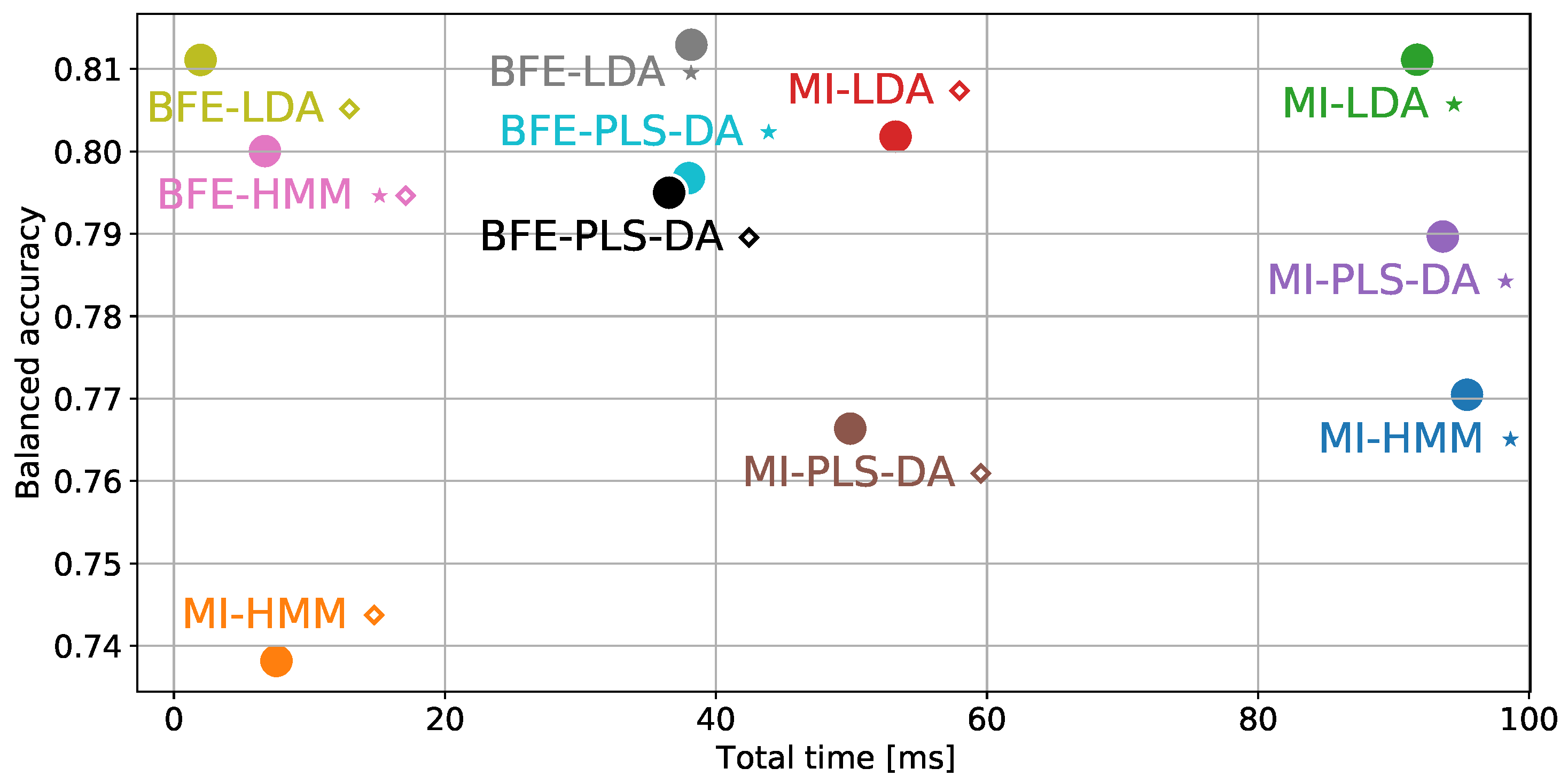


| Feature Selection | Classification | # of Input | Balanced | Time Complexity [ms] | ||
|---|---|---|---|---|---|---|
| Technique | Method | Features | Accuracy | Extraction | Inference | Total |
| MI | HMM ⋆ | 42 | 0.77 | |||
| HMM ⋄ | 22 | 0.74 | ||||
| LDA ⋆ | 42 | 0.81 | ||||
| LDA ⋄ | 27 | 0.80 | ||||
| PLS-DA ⋆ Projected to 22 features | 42 | 0.79 | ||||
| PLS-DA ⋄ Projected to 7 features | 27 | 0.77 | ||||
| BFE | HMM | 12 | 0.80 | |||
| LDA ⋆ | 27 | 0.81 | ||||
| LDA⋄ | 7 | 0.81 | ||||
| PLS-DA ⋆ Projected to 12 features | 22 | 0.80 | ||||
| PLS-DA ⋄ Projected to 7 features | 17 | 0.79 | ||||
| Test Steer | Balanced Accuracy | Precision | Recall |
|---|---|---|---|
| #1 | 0.82 | 0.86 | 0.85 |
| #2 | 0.86 | 0.90 | 0.87 |
| #3 | 0.80 | 0.89 | 0.79 |
| Average | 0.83 ± 0.03 | 0.88 ± 0.02 | 0.83 ± 0.04 |
Publisher’s Note: MDPI stays neutral with regard to jurisdictional claims in published maps and institutional affiliations. |
© 2022 by the authors. Licensee MDPI, Basel, Switzerland. This article is an open access article distributed under the terms and conditions of the Creative Commons Attribution (CC BY) license (https://creativecommons.org/licenses/by/4.0/).
Share and Cite
Pavlovic, D.; Czerkawski, M.; Davison, C.; Marko, O.; Michie, C.; Atkinson, R.; Crnojevic, V.; Andonovic, I.; Rajovic, V.; Kvascev, G.; et al. Behavioural Classification of Cattle Using Neck-Mounted Accelerometer-Equipped Collars. Sensors 2022, 22, 2323. https://doi.org/10.3390/s22062323
Pavlovic D, Czerkawski M, Davison C, Marko O, Michie C, Atkinson R, Crnojevic V, Andonovic I, Rajovic V, Kvascev G, et al. Behavioural Classification of Cattle Using Neck-Mounted Accelerometer-Equipped Collars. Sensors. 2022; 22(6):2323. https://doi.org/10.3390/s22062323
Chicago/Turabian StylePavlovic, Dejan, Mikolaj Czerkawski, Christopher Davison, Oskar Marko, Craig Michie, Robert Atkinson, Vladimir Crnojevic, Ivan Andonovic, Vladimir Rajovic, Goran Kvascev, and et al. 2022. "Behavioural Classification of Cattle Using Neck-Mounted Accelerometer-Equipped Collars" Sensors 22, no. 6: 2323. https://doi.org/10.3390/s22062323
APA StylePavlovic, D., Czerkawski, M., Davison, C., Marko, O., Michie, C., Atkinson, R., Crnojevic, V., Andonovic, I., Rajovic, V., Kvascev, G., & Tachtatzis, C. (2022). Behavioural Classification of Cattle Using Neck-Mounted Accelerometer-Equipped Collars. Sensors, 22(6), 2323. https://doi.org/10.3390/s22062323