
Discussion of the Influence of Multiscale PCA Denoising Methods with Three Different Features


Abstract
:1. Introduction
2. Materials and Methods
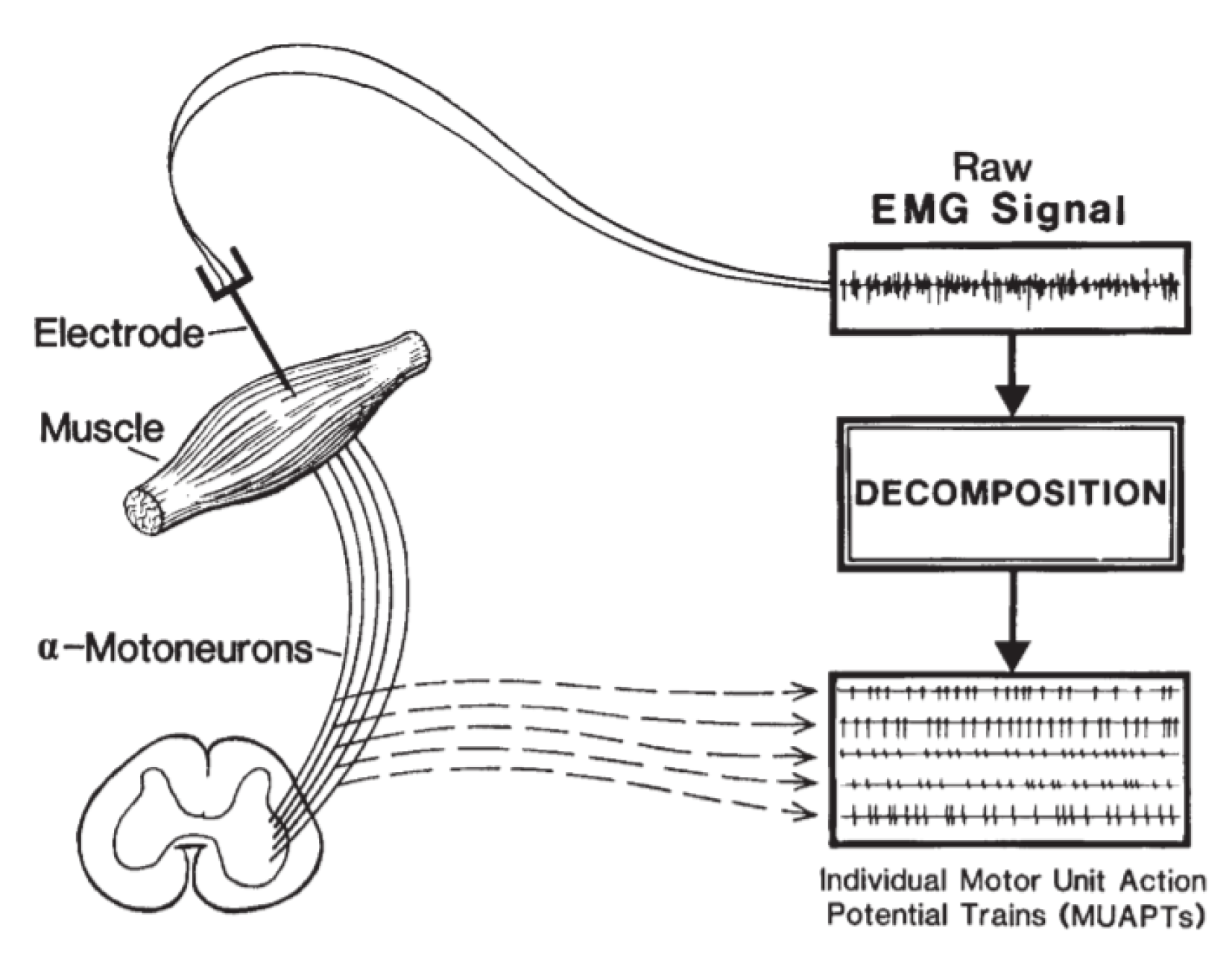
2.1. EMG Signal Components
2.2. Noise and Denoising
2.2.1. Noising
2.2.2. MPCA Denoising
- Use wavelet transformation to transform each channel of the EMG signal to the L of the decomposition level, and collect all the wavelet details in each channel into matrix and the wavelet approximations into matrix .
- Eigen-decompose the covariance matrix of each wavelet matrix, determine the eigenvector and eigenvalue of each, and then arrange them in descending order. The eigenvalues that select the threshold will determine the number of principal components that form a new matrix.
- The relevance factor (when two statistics, namely, statistic and SPE statistic, exceed the control limits, otherwise, 0) will select the nonsignificant scale and form a new EMG signal:
2.3. Raw EMG Signal Processing
2.3.1. Independent Component Decomposition
2.3.2. Wavelet Transform
- ;
- ;
- ;
- ;
- , which make become orthogonal.
2.4. Feature Extraction Method
2.4.1. Autoregression Coefficient
2.4.2. The Decomposition Coefficient Features
2.5. Classification Method
2.5.1. The K-Nearest Neighbor
2.5.2. The Naïve Bayesian
3. Experiment
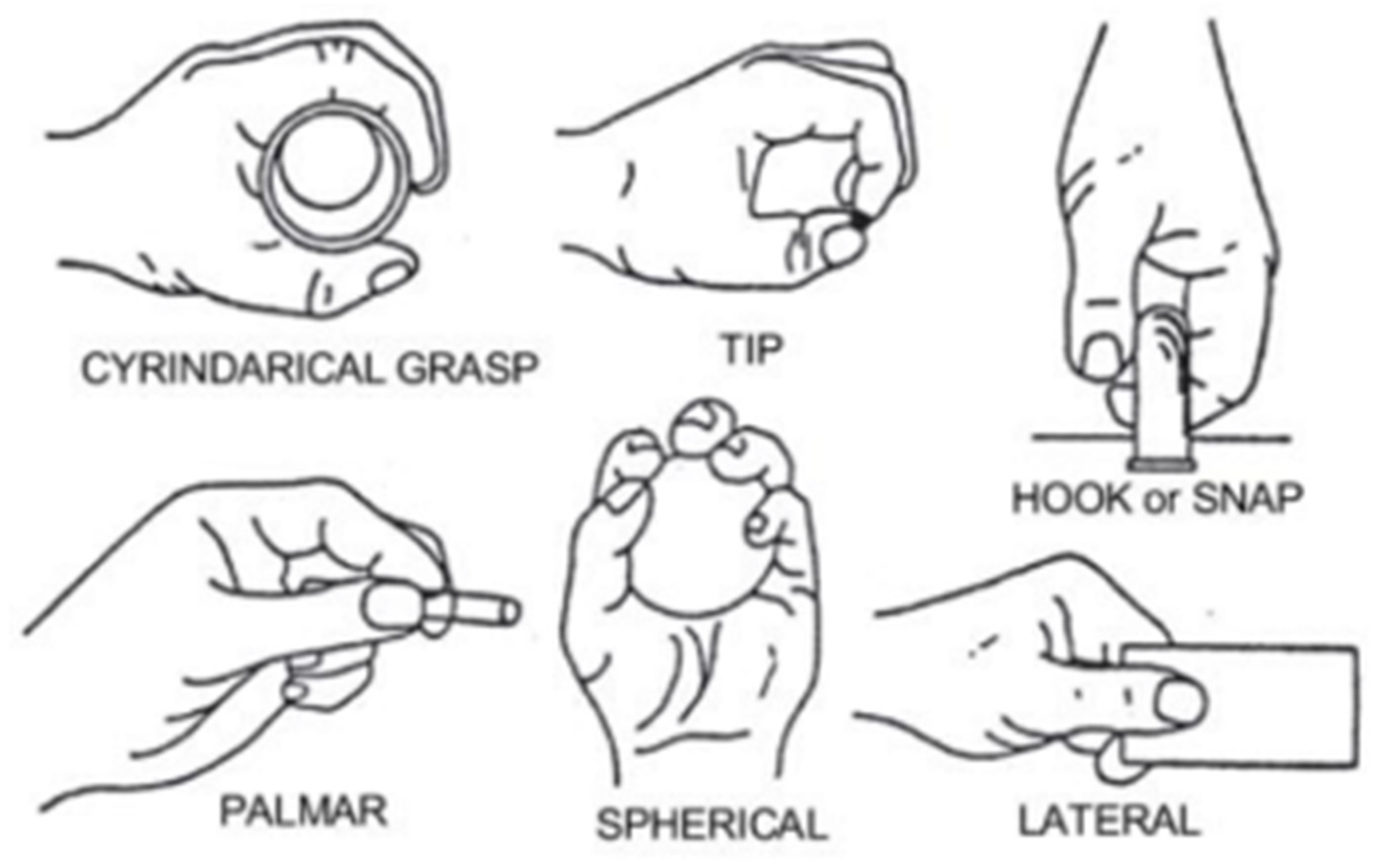
3.1. The Dataset Used
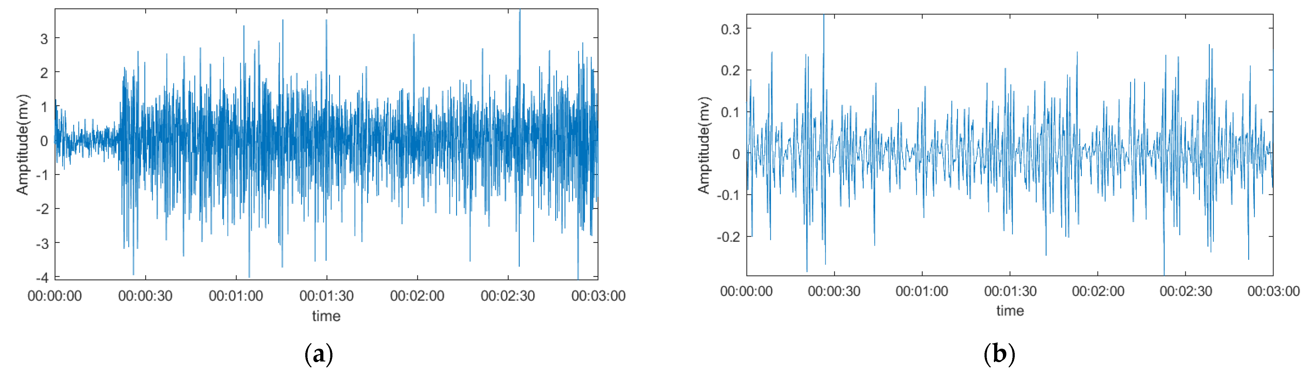
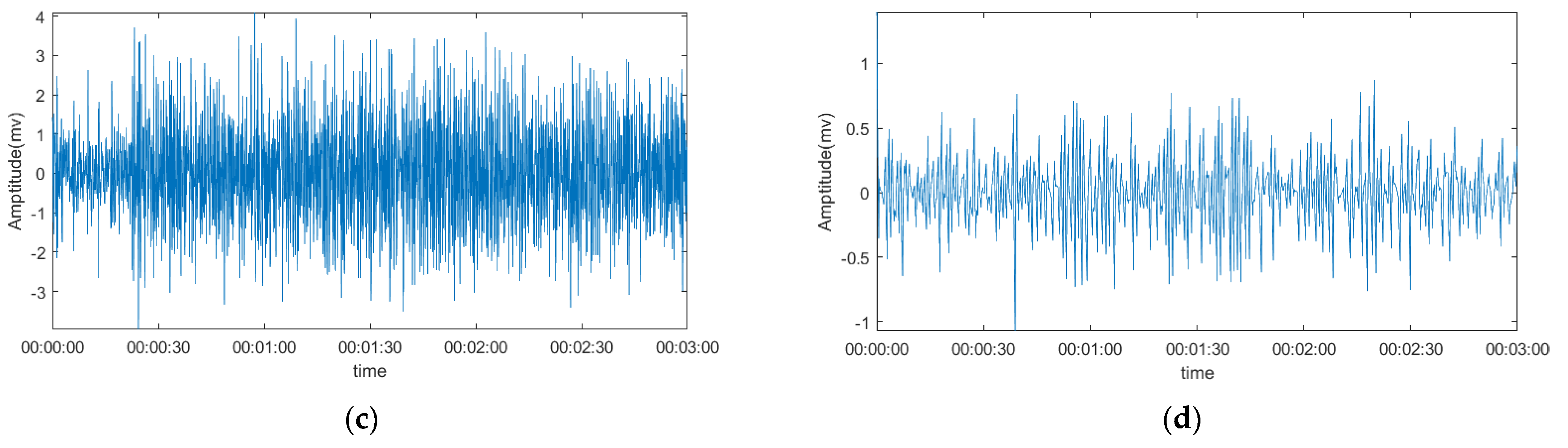
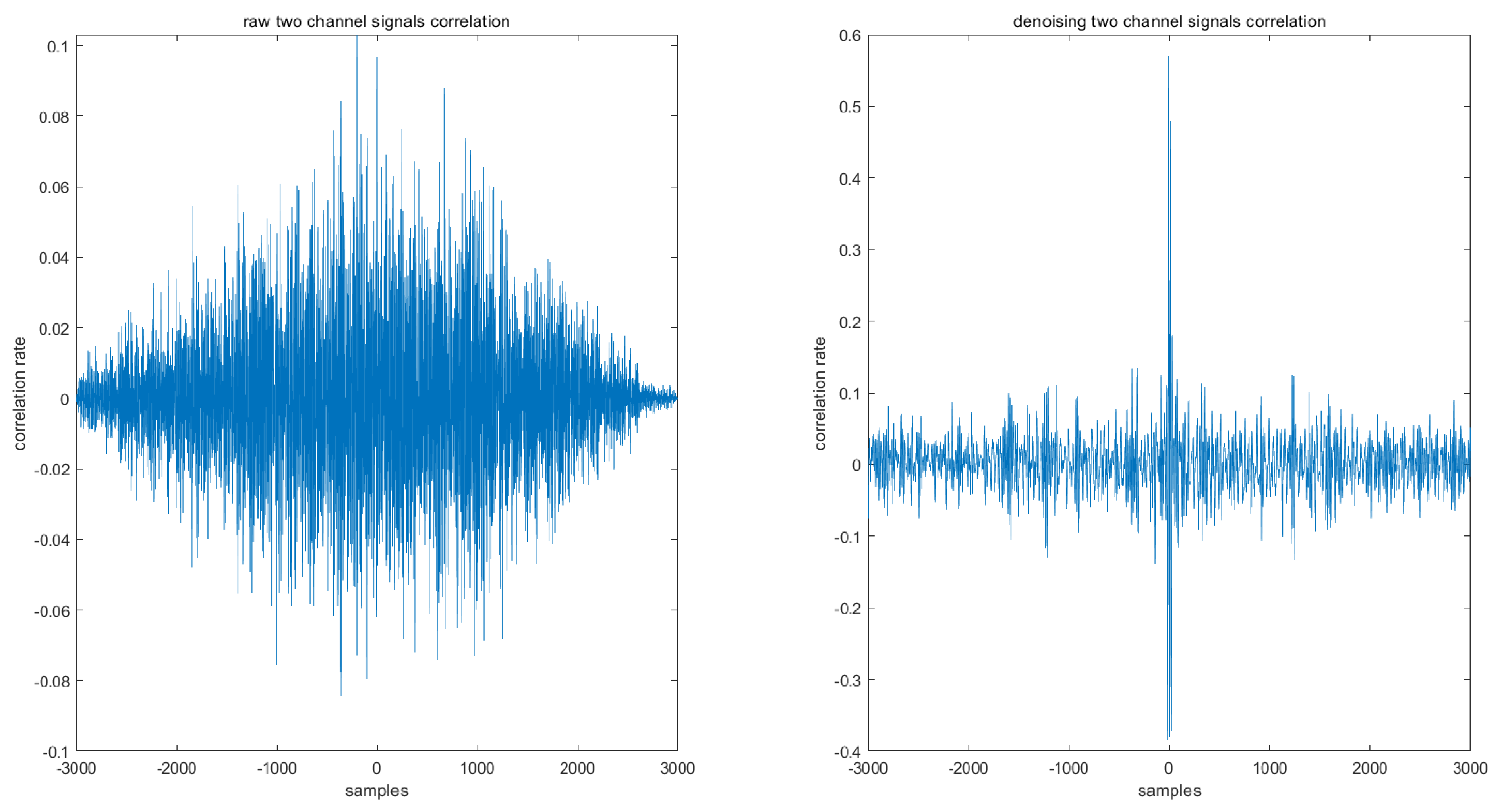
3.2. Comparison of The Denoising Signal and Original Signal
3.3. Signal Decomposition
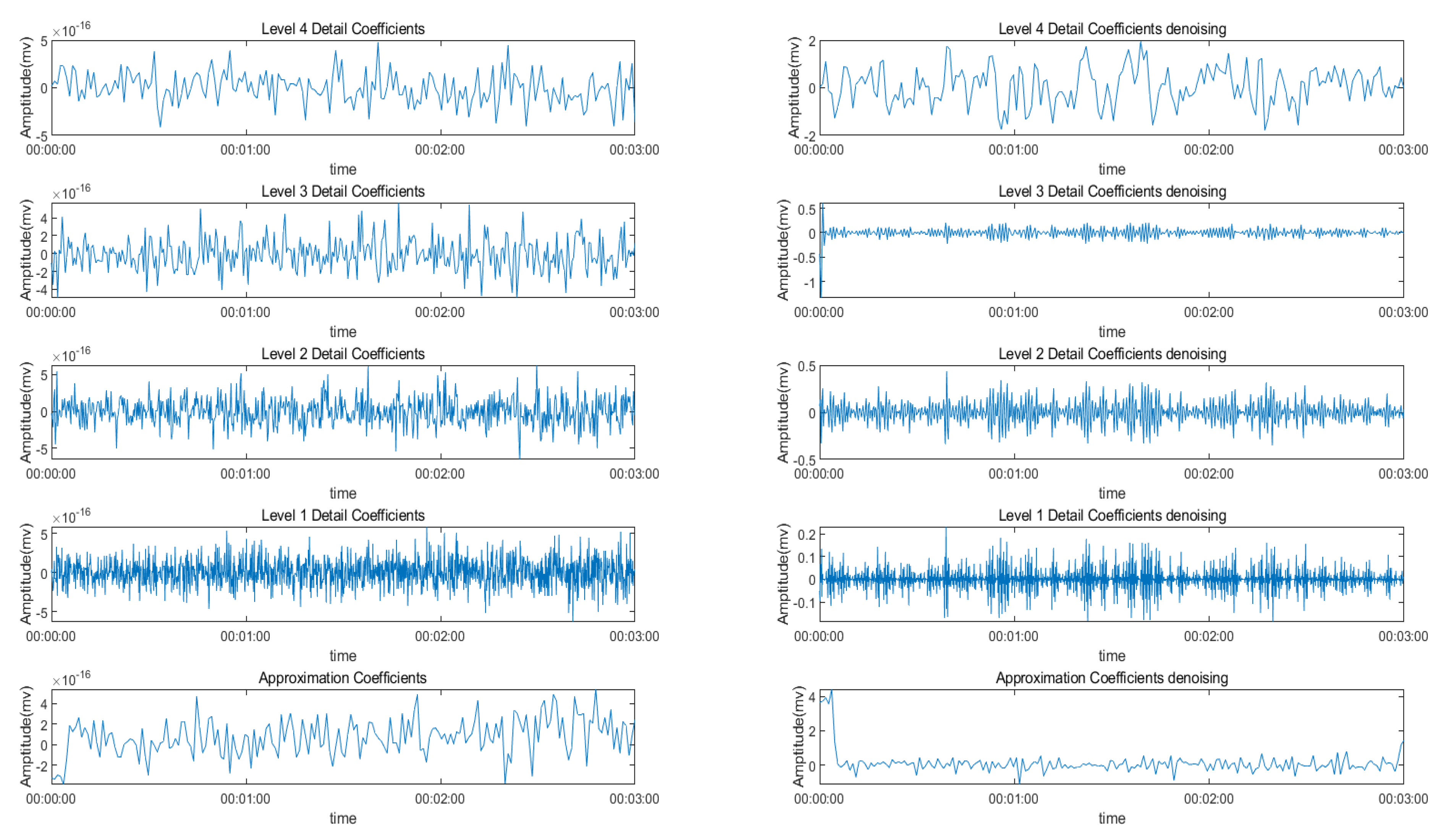
3.3.1. Wavelet Decomposition
3.3.2. ICA Decomposition
3.4. Features
3.5. Classification
4. Discussion
Author Contributions
Funding
Data Availability Statement
Acknowledgments
Conflicts of Interest
References
- Pauk, J. Different techniques for EMG signal processing. J. Vibroeng. 2008, 10, 419. [Google Scholar]
- Reaz, M.B.I.; Hussain, M.S.; Mohd-Yasin, F. Techniques of EMG signal analysis: Detection, processing, classification and applications. Biol. Proced. Online 2006, 8, 11–35. [Google Scholar] [CrossRef] [PubMed] [Green Version]
- Yousefi, J.; Andrew, H.-W. Characterizing EMG data using machine-learning tools. Comput. Biol. Med. 2014, 51, 1–13. [Google Scholar] [CrossRef] [PubMed]
- Hutten, G.J.; van Thuijl, H.F.; van Bellegem, A.C.M.; van Eykern, L.A.; van Aalderen, W.M.C. A literature review of the methodology of EMG recordings of the diaphragm. J. Electromyogr. Kinesiol. 2010, 20, 185–190. [Google Scholar] [CrossRef]
- Negro, F.; Muceli, S.; Castronovo, A.M.; Holobar, A.; Farina, D. Multi-channel intramuscular and surface EMG decomposition by convolutive blind source separation. J. Neural Eng. 2016, 13, 026027. [Google Scholar] [CrossRef]
- Chang, W.X. LMS Algorithm Based on C-expansion of Quaternion. Signal Process. 2011, 27, 1515–1519. [Google Scholar]
- Dan, S. EMG signal decomposition: How can it be accomplished and used? J. Electromyogr. Kinesiol. 2001, 11, 151–173. [Google Scholar]
- Chowdhury, R.H.; Reaz, M.B.I.; Ali, M.A.B.M.; Bakar, A.A.A.; Chellappan, K.; Chang, T.G. Surface Electromyography Signal Processing and Classification Techniques. Sensors 2013, 13, 12431–12466. [Google Scholar] [CrossRef]
- Akinwumi, A.A.; Gorban, A.N. Multiscale principal component analysis. J. Phys. 2014, 490, 12081. [Google Scholar]
- Gokgoz, E.; Subasi, A. Effect of multiscale PCA de-noising on EMG signal classification for diagnosis of neuromuscular disorders. J. Med. Syst. 2014, 38, 31. [Google Scholar] [CrossRef]
- Xu, Z.; Yu, W.; Han, R. Wavelet transform theory and its application in EMG signal processing. In Proceedings of the IEEE Seventh International Conference on Fuzzy Systems & Knowledge Discovery, Yantai, China, 10–12 August 2010. [Google Scholar]
- Wang, G.; Zhang, Y.; Liu, C.; Xie, Q.; Xu, Y. A new tool wear monitoring method based on multi-scale PCA. J. Intell. Manuf. 2019, 30, 113–122. [Google Scholar] [CrossRef]
- Sharma, L.N.; Danadapat, S.; Mahanta, A. Abstract-multiscale multiscale PCA based quality controlled denoising of multichannel ECG signals. Int. J. Inf. Electron. Eng. 2017, 2, 107–111. [Google Scholar]
- García, G.A.; Maekawa, K.; Akazawa, K. Decomposition of Synthetic Multi-channel Surface-Electromyogram Using Independent Component Analysis. In Proceedings of the International Conference on Independent Component Analysis and Signal Separation, Granada, Spain, 22–24 September 2004; pp. 985–992. [Google Scholar]
- Chawla, M.P.S. A comparative analysis of principal component and independent component techniques for electrocardiograms. Neural Comput. Appl. 2009, 18, 539–556. [Google Scholar] [CrossRef]
- Shi, Z.; Tang, H.; Tang, Y. A fast fixed-point algorithm for complexity pursuit. Neurocomputing 2005, 64, 529–536. [Google Scholar] [CrossRef]
- Phinyomark, A.; Quaine, F.; Charbonnier, S.; Serviere, C.; Tarpin-Bernard, F.; Laurillau, Y. EMG feature evaluation for improving myoelectric pattern recognition robustness. Expert Syst. Appl. 2013, 40, 4832–4840. [Google Scholar] [CrossRef]
- Phinyomark, A.; Pornchai, P.; Chusak, L. Feature reduction and selection for EMG signal classification. Expert Syst. Appl. 2012, 39, 7420–7431. [Google Scholar] [CrossRef]
- Paiss, O.; Inbar, G.F. Autoregressive modeling of surface EMG and its spectrum with application to fatigue. Math. Comput. Model. 1987, 10, 793–794. [Google Scholar] [CrossRef]
- Ramírez-Martínez, D.; Alfaro-Ponce, M.; Pogrebnyak, O.; Aldape-Pérez, M.; Argüelles-Cruz, A.-J. Hand Movement Classification Using Burg Reflection Coefficients. Sensors 2019, 19, 475. [Google Scholar] [CrossRef] [Green Version]
- Brockwell, P.J.; Dahlhaus, R. Generalized Levinson–Durbin and Burg algorithms. J. Econom. 2004, 118, 129–149. [Google Scholar] [CrossRef]
- Hamilton-Wright, A.; McLean, L.; Stashuk, D.W.; Calder, K.M. Bayesian aggregation versus majority vote in the characterization of non-specific arm pain based on quantitative needle electromyography. J. Neuroeng. Rehabil. 2010, 7, 8. [Google Scholar] [CrossRef] [Green Version]
- Gokgoz, E.; Abdulhamit, S. Comparison of decision tree algorithms for EMG signal classification using DWT. Biomed. Signal Process. Control 2015, 18, 138–144. [Google Scholar] [CrossRef]
- Al-Faiz, M.Z.; Ali, A.A.; Miry, A.H. A k-nearest neighbor based algorithm for human arm movements recognition using EMG signals. In Proceedings of the IEEE International Conference on Energy, Manama, Bahrain, 18–21 December 2010. [Google Scholar]
- Rasheed, S.; Stashuk, D.; Kamel, M. Adaptive fuzzy k-NN classifier for EMG signal decomposition. Med. Eng. Phys. 2006, 28, 694–709. [Google Scholar] [CrossRef] [PubMed]
- Sapsanis, C.; Georgoulas, G.; Tzes, A.; Lymberopoulos, D. Improving EMG based classification of basic hand movements using EMD. In Proceedings of the 35th Annual International Conference of the IEEE Engineering in Medicine and Biology Society (EMBC 13), Osaka, Japan, 3–7 July 2013; pp. 5754–5757. [Google Scholar]
- UCL, sEMG for Basic Hand Movements Data Set. Available online: http://archive.ics.uci.edu/ml/datasets/sEMG+for+Basic+Hand+movements# (accessed on 14 September 2020).
- Chowdhury, A.; Raza, H.; Meena, Y.K.; Dutta, A.; Prasad, G. EEG-EMG correlation-based brain-computer interface for hand orthosis supported neuro-rehabilitation. J. Neurosci. Methods 2019, 312, 1–11. [Google Scholar] [CrossRef] [PubMed] [Green Version]


| Features | Multiscale PCA Denoising | Original Signal | ||||||
|---|---|---|---|---|---|---|---|---|
| k = 1 | k = 4 | k = 7 | k = 10 | k = 1 | k = 4 | k = 7 | k = 10 | |
| WT coefficient | 100% | 80.27% | 46.77% | 53.33% | 100% | 85.05% | 65% | 74.5% |
| ICA coefficient | 53.66% | 47.88% | 48.16% | 46.61% | 42.27% | 38.16% | 36.33% | 33.05% |
| Autoregression coefficient | 33.72% | 33.27% | 34.44% | 31.88% | 69.11% | 72.38% | 73.88% | 73% |
| Features | Multiscale PCA Denoising | |||
|---|---|---|---|---|
| k = 1 | k = 4 | k = 7 | k = 10 | |
| WT coefficient | 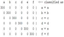 | 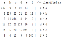 |  |  |
| ICA coefficient | 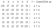 | 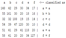 |  |  |
| Autoregression coefficient |  | 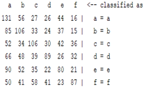 |  | 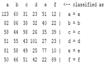 |
| Features | Original Signal | |||
|---|---|---|---|---|
| k = 1 | k = 4 | k = 7 | k = 10 | |
| WT coefficient | 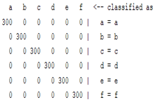 | 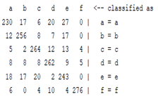 |  |  |
| ICA coefficient | 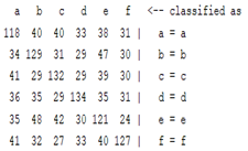 | 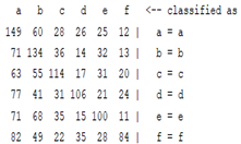 | 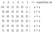 |  |
| Autoregression coefficient |  | 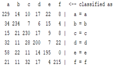 | 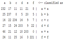 |  |
| Features | Multiscale PCA Denoising | Original Signal |
|---|---|---|
| WT coefficient | 22.72% | 46% |
| ICA coefficient | 15.27% | 8.27% |
| Autoregression coefficient | 22.38% | 43.5% |
| Features | Multiscale PCA Denoising | Original Signal |
|---|---|---|
| WT coefficient |  |  |
| ICA coefficient | 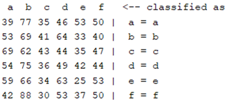 | 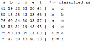 |
| Autoregression coefficient | 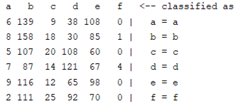 | 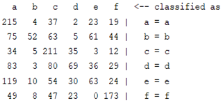 |
Publisher’s Note: MDPI stays neutral with regard to jurisdictional claims in published maps and institutional affiliations. |
© 2022 by the authors. Licensee MDPI, Basel, Switzerland. This article is an open access article distributed under the terms and conditions of the Creative Commons Attribution (CC BY) license (https://creativecommons.org/licenses/by/4.0/).
Share and Cite
Zhang, C.; Sun, T. Discussion of the Influence of Multiscale PCA Denoising Methods with Three Different Features. Sensors 2022, 22, 1604. https://doi.org/10.3390/s22041604
Zhang C, Sun T. Discussion of the Influence of Multiscale PCA Denoising Methods with Three Different Features. Sensors. 2022; 22(4):1604. https://doi.org/10.3390/s22041604
Chicago/Turabian StyleZhang, Chizhou, and Tao Sun. 2022. "Discussion of the Influence of Multiscale PCA Denoising Methods with Three Different Features" Sensors 22, no. 4: 1604. https://doi.org/10.3390/s22041604
APA StyleZhang, C., & Sun, T. (2022). Discussion of the Influence of Multiscale PCA Denoising Methods with Three Different Features. Sensors, 22(4), 1604. https://doi.org/10.3390/s22041604