
GAN-Based Image Colorization for Self-Supervised Visual Feature Learning

 ,
,  ,
,  ,
,  and
and
Abstract
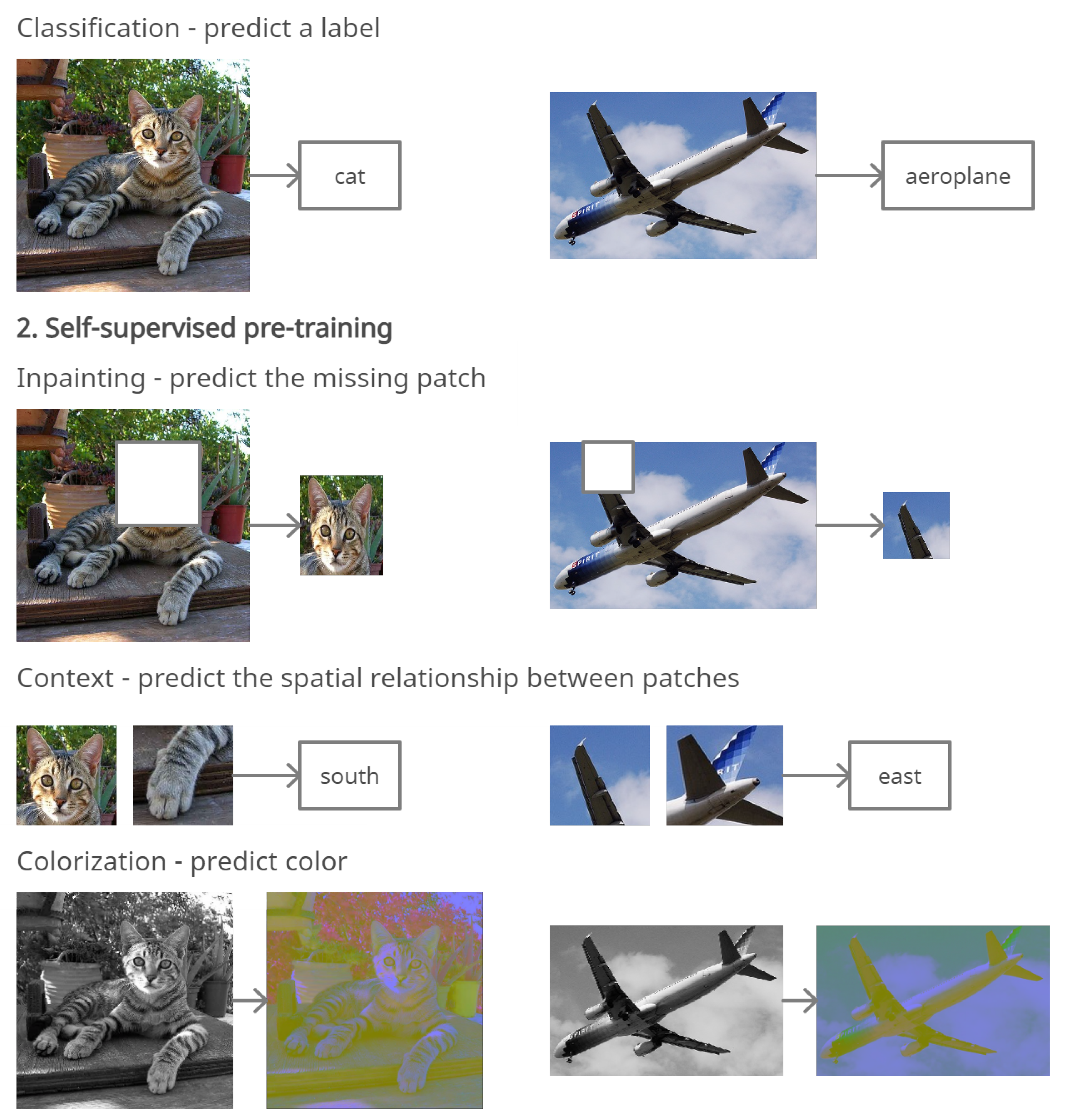
:1. Introduction
2. Related Work
3. Methods
3.1. Image Colorization
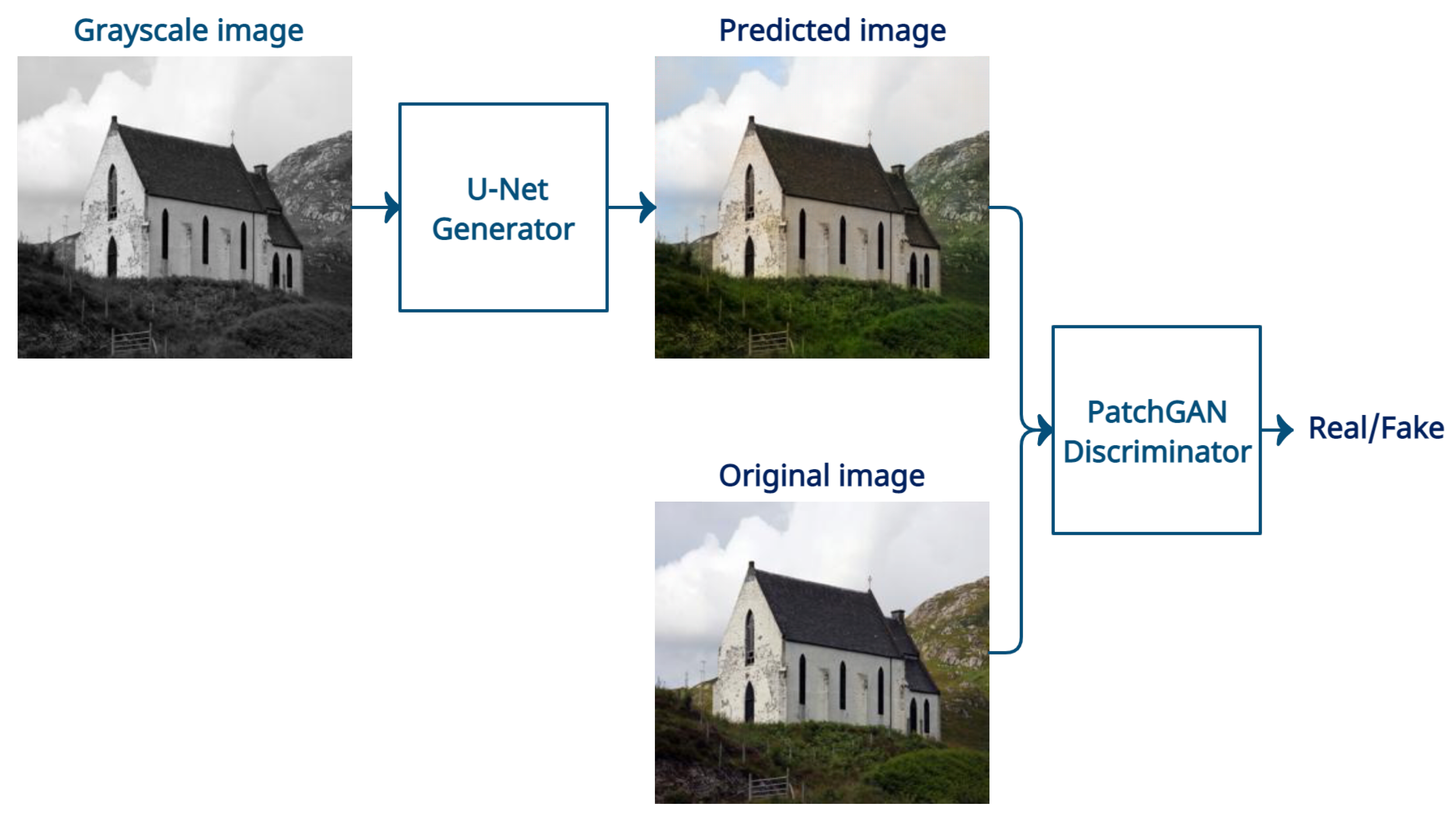
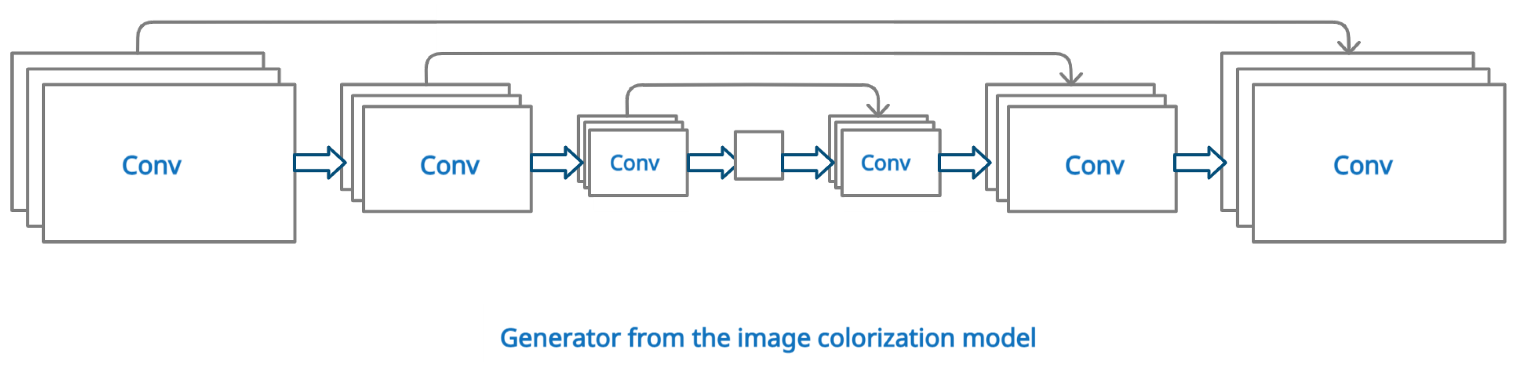
3.2. Generative Adversarial Networks for Image Colorization
3.3. Image Colorization Model
3.3.1. Dataset
3.3.2. Color Space
3.3.3. Objective Function
3.3.4. Metrics for Evaluating Image Colorization Methods
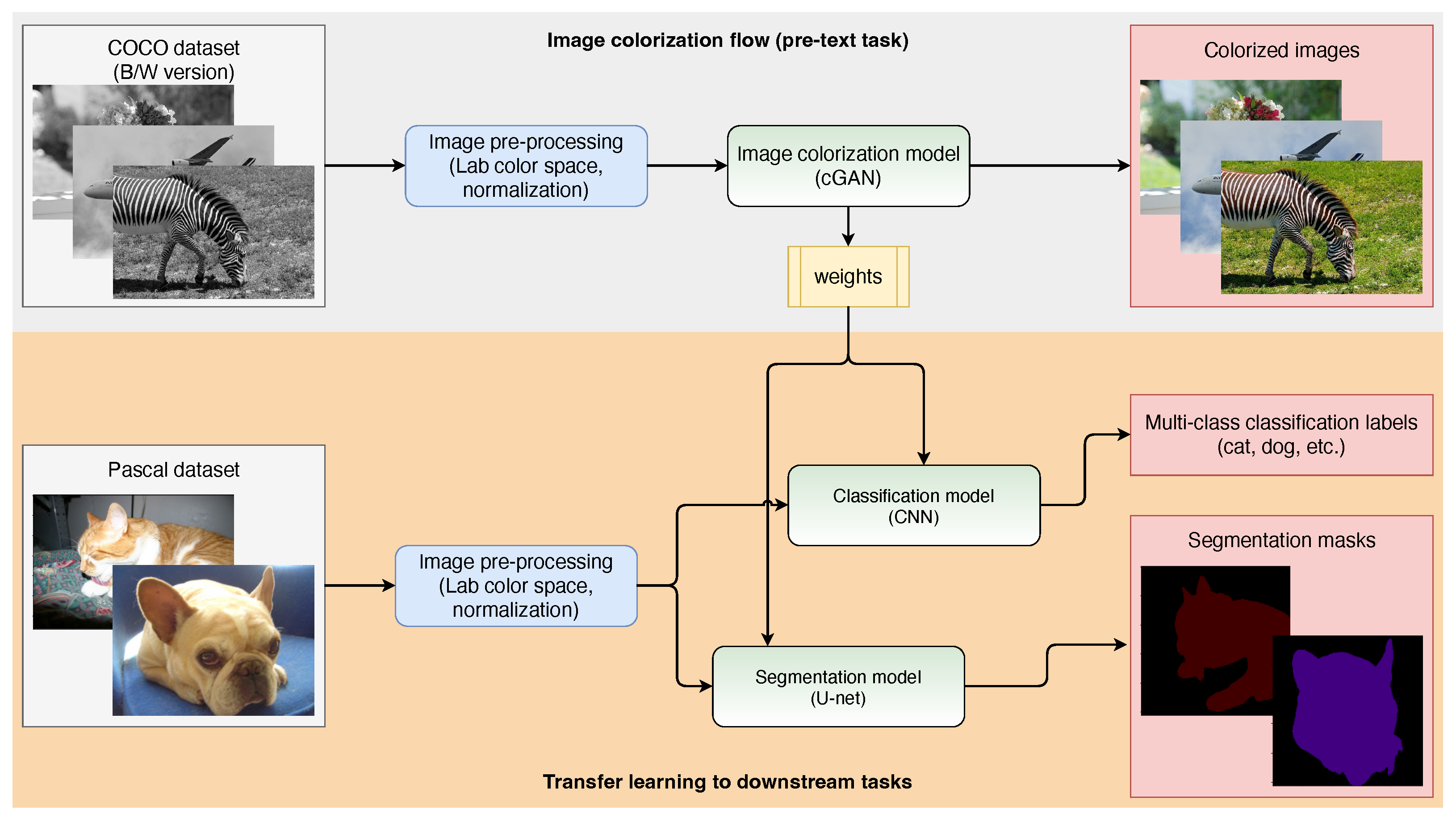
3.4. Transfer Learning to Downstream Tasks
3.4.1. Dataset
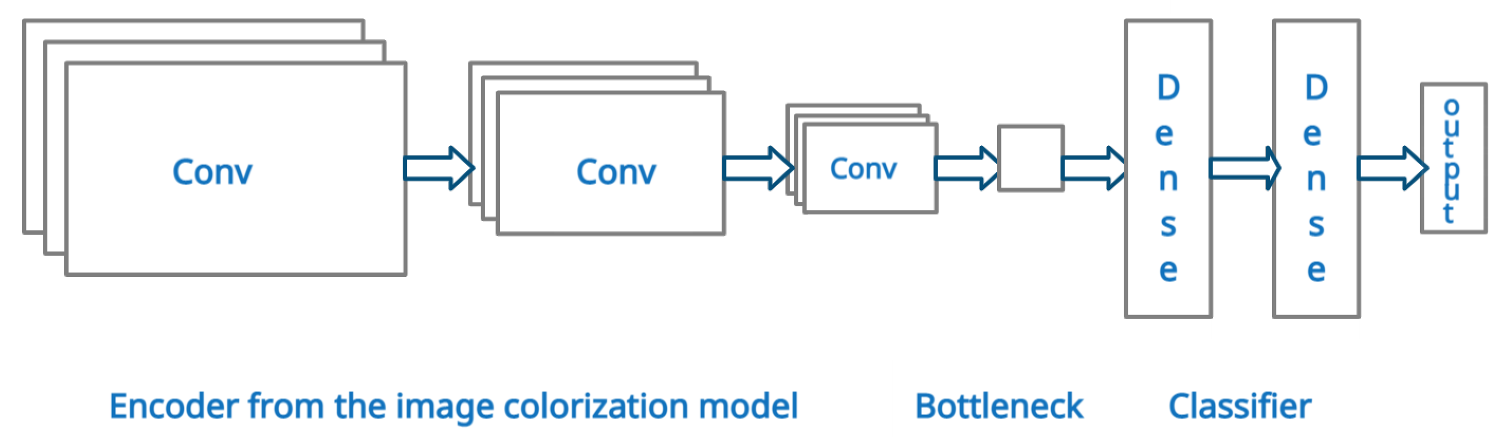
3.4.2. Multilabel Image Classification Model
3.4.3. Semantic Segmentation Model
4. Results
4.1. Image Colorization
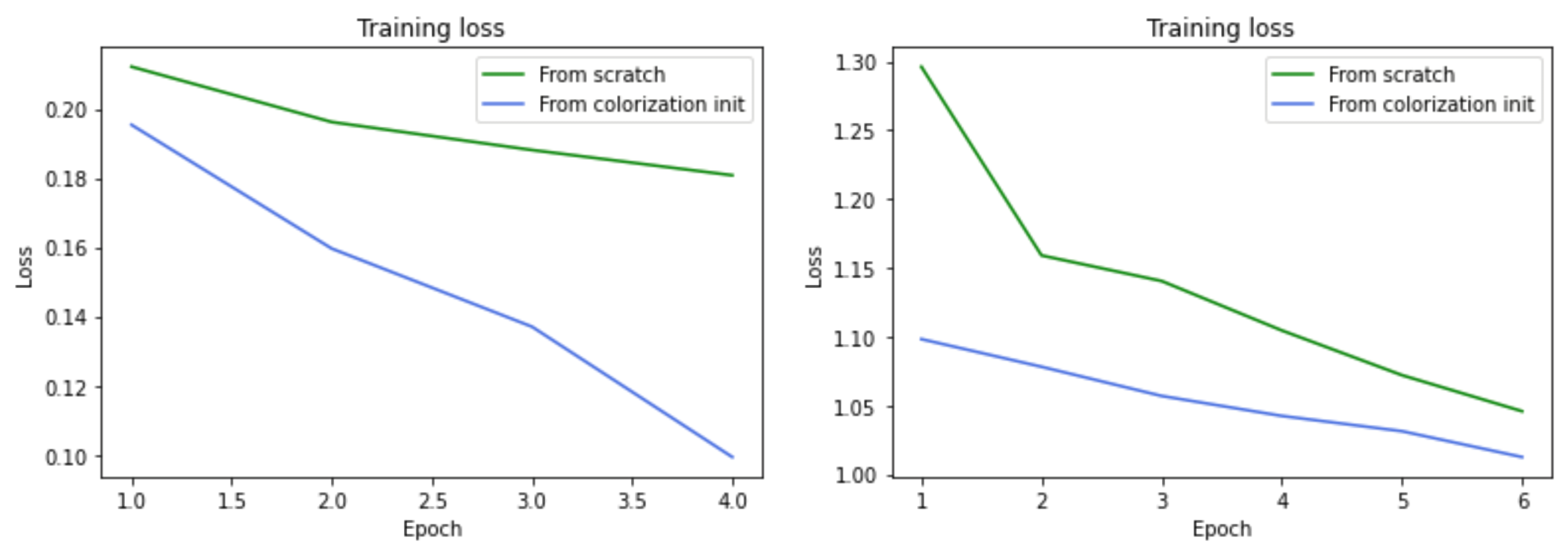
4.2. Multilabel Classification
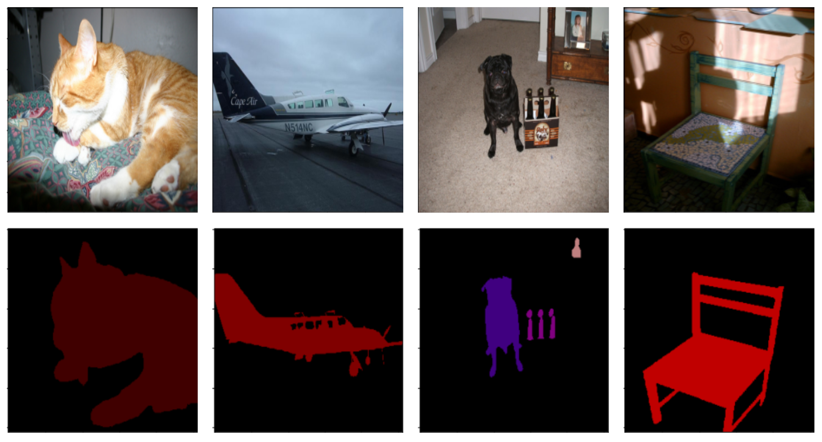
4.3. Semantic Segmentation
5. Discussion
6. Conclusions
Author Contributions
Funding
Institutional Review Board Statement
Informed Consent Statement
Data Availability Statement
Acknowledgments
Conflicts of Interest
References
- Russakovsky, O.; Deng, J.; Su, H.; Krause, J.; Satheesh, S.; Ma, S.; Huang, Z.; Karpathy, A.; Khosla, A.; Bernstein, M.; et al. Imagenet large scale visual recognition challenge. Int. J. Comput. Vis. 2015, 115, 211–252. [Google Scholar] [CrossRef] [Green Version]
- Girshick, R. Fast r-cnn. In Proceedings of the IEEE International Conference on Computer Vision, Santiago, Chile, 7–13 December 2015; pp. 1440–1448. [Google Scholar]
- Ren, S.; He, K.; Girshick, R.; Sun, J. Faster r-cnn: Towards real-time object detection with region proposal networks. Adv. Neural Inf. Process. Syst. 2015, 28, 91–99. [Google Scholar] [CrossRef] [PubMed] [Green Version]
- Chen, L.C.; Papandreou, G.; Kokkinos, I.; Murphy, K.; Yuille, A.L. Deeplab: Semantic image segmentation with deep convolutional nets, atrous convolution, and fully connected crfs. IEEE Trans. Pattern Anal. Mach. Intell. 2017, 40, 834–848. [Google Scholar] [CrossRef] [PubMed] [Green Version]
- He, K.; Gkioxari, G.; Dollár, P.; Girshick, R. Mask r-cnn. In Proceedings of the IEEE International Conference on Computer Vision, Venice, Italy, 22–29 October 2017; pp. 2961–2969. [Google Scholar]
- Vinyals, O.; Toshev, A.; Bengio, S.; Erhan, D. Show and tell: A neural image caption generator. In Proceedings of the IEEE Conference on Computer Vision and Pattern Recognition, Boston, MA, USA, 7–12 June 2015; pp. 3156–3164. [Google Scholar]
- Deng, J.; Dong, W.; Socher, R.; Li, L.J.; Li, K.; Li, F.-F. Imagenet: A large-scale hierarchical image database. In Proceedings of the 2009 IEEE Conference on Computer Vision and Pattern Recognition, Miami, FL, USA, 20–25 June 2009; pp. 248–255. [Google Scholar]
- Lin, T.Y.; Maire, M.; Belongie, S.; Hays, J.; Perona, P.; Ramanan, D.; Dollár, P.; Zitnick, C.L. Microsoft coco: Common objects in context. In Proceedings of the European Conference on Computer Vision, Zurich, Switzerland, 6–12 September 2014; pp. 740–755. [Google Scholar]
- Everingham, M.; Van Gool, L.; Williams, C.K.; Winn, J.; Zisserman, A. The pascal visual object classes (voc) challenge. Int. J. Comput. Vis. 2010, 88, 303–338. [Google Scholar] [CrossRef] [Green Version]
- Zhou, B.; Lapedriza, A.; Khosla, A.; Oliva, A.; Torralba, A. Places: A 10 million image database for scene recognition. IEEE Trans. Pattern Anal. Mach. Intell. 2017, 40, 1452–1464. [Google Scholar] [CrossRef] [Green Version]
- Torrey, L.; Shavlik, J. Transfer learning. Handbook of Research on Machine Learning Applications. IGI Glob. 2009, 3, 17–35. [Google Scholar]
- Beyer, L.; Hénaff, O.J.; Kolesnikov, A.; Zhai, X.; van den Oord, A. Are we done with imagenet? arXiv 2020, arXiv:2006.07159. [Google Scholar]
- Jing, L.; Tian, Y. Self-supervised visual feature learning with deep neural networks: A survey. IEEE Trans. Pattern Anal. Mach. Intell. 2020, 43, 4037–4058. [Google Scholar] [CrossRef]
- Pathak, D.; Krahenbuhl, P.; Donahue, J.; Darrell, T.; Efros, A.A. Context encoders: Feature learning by inpainting. In Proceedings of the IEEE conference on Computer Vision and Pattern Recognition, Las Vegas, NV, USA, 27–30 June 2016; pp. 2536–2544. [Google Scholar]
- Ledig, C.; Theis, L.; Huszár, F.; Caballero, J.; Cunningham, A.; Acosta, A.; Aitken, A.; Tejani, A.; Totz, J.; Wang, Z.; et al. Photo-realistic single image super-resolution using a generative adversarial network. In Proceedings of the IEEE Conference on Computer Vision and Pattern Recognition, Honolulu, HI, USA, 21–26 July 2017; pp. 4681–4690. [Google Scholar]
- Zhang, R.; Isola, P.; Efros, A.A. Colorful image colorization. In Proceedings of the European Conference on Computer Vision, Amsterdam, The Netherlands, 11–14 October 2016; pp. 649–666. [Google Scholar]
- Mirza, M.; Osindero, S. Conditional generative adversarial nets. arXiv 2014, arXiv:1411.1784. [Google Scholar]
- Tsoumakas, G.; Katakis, I. Multi-label classification: An overview. Int. J. Data Warehous. Min. (IJDWM) 2007, 3, 1–13. [Google Scholar] [CrossRef] [Green Version]
- Thoma, M. A survey of semantic segmentation. arXiv 2016, arXiv:1602.06541. [Google Scholar]
- Noroozi, M.; Vinjimoor, A.; Favaro, P.; Pirsiavash, H. Boosting self-supervised learning via knowledge transfer. In Proceedings of the IEEE Conference on Computer Vision and Pattern Recognition, Salt Lake City, UT, USA, 16–23 June 2018; pp. 9359–9367. [Google Scholar]
- Noroozi, M.; Favaro, P. Unsupervised learning of visual representations by solving jigsaw puzzles. In Proceedings of the European Conference on Computer Vision, Amsterdam, The Netherlands, 11–14 October 2016; pp. 69–84. [Google Scholar]
- Misra, I.; Zitnick, C.L.; Hebert, M. Shuffle and learn: Unsupervised learning using temporal order verification. In Proceedings of the European Conference on Computer Vision, Amsterdam, The Netherlands, 11–14 October 2016; pp. 527–544. [Google Scholar]
- Pathak, D.; Girshick, R.; Dollár, P.; Darrell, T.; Hariharan, B. Learning features by watching objects move. In Proceedings of the IEEE Conference on Computer Vision and Pattern Recognition, Honolulu, HI, USA, 21–26 July 2017; pp. 2701–2710. [Google Scholar]
- Ren, Z.; Lee, Y.J. Cross-domain self-supervised multi-task feature learning using synthetic imagery. In Proceedings of the IEEE Conference on Computer Vision and Pattern Recognition, Salt Lake City, UT, USA, 16–23 June 2018; pp. 762–771. [Google Scholar]
- Agrawal, P.; Carreira, J.; Malik, J. Learning to see by moving. In Proceedings of the IEEE International Conference on Computer Vision, Santiago, Chile, 7–13 December 2015; pp. 37–45. [Google Scholar]
- Sayed, N.; Brattoli, B.; Ommer, B. Cross and learn: Cross-modal self-supervision. In Proceedings of the German Conference on Pattern Recognition, Stuttgart, Germany, 9–12 October 2018; pp. 228–243. [Google Scholar]
- Korbar, B.; Tran, D.; Torresani, L. Cooperative learning of audio and video models from self-supervised synchronization. arXiv 2018, arXiv:1807.00230. [Google Scholar]
- Li, C.L.; Sohn, K.; Yoon, J.; Pfister, T. Cutpaste: Self-supervised learning for anomaly detection and localization. In Proceedings of the IEEE/CVF Conference on Computer Vision and Pattern Recognition, Nashville, TN, USA, 20–25 June 2021; pp. 9664–9674. [Google Scholar]
- Jin, X.; Chen, Z.; Lin, J.; Chen, Z.; Zhou, W. Unsupervised single image deraining with self-supervised constraints. In Proceedings of the 2019 IEEE International Conference on Image Processing (ICIP), Taipei, Taiwan, 22–25 September 2019; pp. 2761–2765. [Google Scholar]
- Larsson, G.; Maire, M.; Shakhnarovich, G. Learning representations for automatic colorization. In Proceedings of the European Conference on Computer Vision, Amsterdam, The Netherlands, 11–14 October 2016; pp. 577–593. [Google Scholar]
- Larsson, G.; Maire, M.; Shakhnarovich, G. Colorization as a proxy task for visual understanding. In Proceedings of the IEEE Conference on Computer Vision and Pattern Recognition, Honolulu, HI, USA, 21–26 July 2017; pp. 6874–6883. [Google Scholar]
- Zhang, R.; Isola, P.; Efros, A.A. Split-brain autoencoders: Unsupervised learning by cross-channel prediction. In Proceedings of the IEEE Conference on Computer Vision and Pattern Recognition, Honolulu, HI, USA, 21–26 July 2017; pp. 1058–1067. [Google Scholar]
- Isola, P.; Zhu, J.Y.; Zhou, T.; Efros, A.A. Image-to-image translation with conditional adversarial networks. In Proceedings of the IEEE Conference on Computer Vision and Pattern Recognition, Honolulu, HI, USA, 21–26 July 2017; pp. 1125–1134. [Google Scholar]
- Nazeri, K.; Ng, E.; Ebrahimi, M. Image colorization using generative adversarial networks. In Proceedings of the International Conference on Articulated Motion and Deformable Objects, Palma de Mallorca, Spain, 12–13 July 2018; pp. 85–94. [Google Scholar]
- Cao, Y.; Zhou, Z.; Zhang, W.; Yu, Y. Unsupervised diverse colorization via generative adversarial networks. In Proceedings of the Joint European Conference on Machine Learning and Knowledge Discovery in Databases, Skopje, North Macedonia, 18–22 September 2017; pp. 151–166. [Google Scholar]
- Kiani, L.; Saeed, M.; Nezamabadi-pour, H. Image Colorization Using Generative Adversarial Networks and Transfer Learning. In Proceedings of the 2020 International Conference on Machine Vision and Image Processing (MVIP), Qom, Iran, 18–20 February 2020; pp. 1–6. [Google Scholar]
- Deshpande, A.; Rock, J.; Forsyth, D. Learning large-scale automatic image colorization. In Proceedings of the IEEE International Conference on Computer Vision, Santiago, Chile, 7–13 December 2015; pp. 567–575. [Google Scholar]
- Iizuka, S.; Simo-Serra, E.; Ishikawa, H. Let there be color! Joint end-to-end learning of global and local image priors for automatic image colorization with simultaneous classification. ACM Trans. Graph. (ToG) 2016, 35, 1–11. [Google Scholar] [CrossRef]
- Baldassarre, F.; Morín, D.G.; Rodés-Guirao, L. Deep koalarization: Image colorization using cnns and inception-resnet-v2. arXiv 2017, arXiv:1712.03400. [Google Scholar]
- Kalajdjieski, J.; Zdravevski, E.; Corizzo, R.; Lameski, P.; Kalajdziski, S.; Pires, I.M.; Garcia, N.M.; Trajkovik, V. Air Pollution Prediction with Multi-Modal Data and Deep Neural Networks. Remote Sens. 2020, 12, 4142. [Google Scholar] [CrossRef]
- Hosni, R.; Hussein, W. Refined image colorization using capsule generative adversarial networks. In Proceedings of the Twelfth International Conference on Machine Vision (ICMV 2019), Amsterdam, The Netherlands, 6–18 November 2019; International Society for Optics and Photonics: Bellingham, WA, USA, 2020; Volume 11433, p. 114332R. [Google Scholar]
- Vitoria, P.; Raad, L.; Ballester, C. Chromagan: Adversarial picture colorization with semantic class distribution. In Proceedings of the IEEE/CVF Winter Conference on Applications of Computer Vision, Snowmass Village, CO, USA, 1–5 March 2020; pp. 2445–2454. [Google Scholar]
- Yoo, S.; Bahng, H.; Chung, S.; Lee, J.; Chang, J.; Choo, J. Coloring with limited data: Few-shot colorization via memory augmented networks. In Proceedings of the IEEE/CVF Conference on Computer Vision and Pattern Recognition, Long Beach, CA, USA, 15–20 June 2019; pp. 11283–11292. [Google Scholar]
- Du, K.; Liu, C.; Cao, L.; Guo, Y.; Zhang, F.; Wang, T. Double-Channel Guided Generative Adversarial Network for Image Colorization. IEEE Access 2021, 9, 21604–21617. [Google Scholar] [CrossRef]
- Ronneberger, O.; Fischer, P.; Brox, T. U-net: Convolutional networks for biomedical image segmentation. In Proceedings of the International Conference on Medical Image Computing and Computer-Assisted Intervention, Munich, Germany, 5–9 October 2015; pp. 234–241. [Google Scholar]
- Wang, Z.; Bovik, A.C.; Sheikh, H.R.; Simoncelli, E.P. Image quality assessment: From error visibility to structural similarity. IEEE Trans. Image Process. 2004, 13, 600–612. [Google Scholar] [CrossRef] [Green Version]
- Lateef, F.; Ruichek, Y. Survey on semantic segmentation using deep learning techniques. Neurocomputing 2019, 338, 321–348. [Google Scholar] [CrossRef]
- Treneska, S. Image Colorization. 2021. Available online: https://github.com/sandratreneska/Image-colorization (accessed on 26 January 2022).
- Treneska, S. Self-Supervised Visual Feature Learning. 2021. Available online: https://github.com/sandratreneska/Self-supervised-visual-feature-learning (accessed on 26 January 2022).
- Lameski, J.; Jovanov, A.; Zdravevski, E.; Lameski, P.; Gievska, S. Skin lesion segmentation with deep learning. In Proceedings of the IEEE EUROCON 2019-18th International Conference on Smart Technologies, Novi Sad, Serbia, 1–4 July 2019; pp. 1–5. [Google Scholar]
- Aresta, G.; Jacobs, C.; Araújo, T.; Cunha, A.; Ramos, I.; van Ginneken, B.; Campilho, A. iW-Net: An automatic and minimalistic interactive lung nodule segmentation deep network. Sci. Rep. 2019, 9, 11591. [Google Scholar] [CrossRef] [Green Version]
- Zdravevski, E.; Lameski, P.; Apanowicz, C.; Slezak, D. From Big Data to business analytics: The case study of churn prediction. Appl. Soft Comput. 2020, 90, 106164. [Google Scholar] [CrossRef]
- Grzegorowski, M.; Zdravevski, E.; Janusz, A.; Lameski, P.; Apanowicz, C.; Slezak, D. Cost optimization for big data workloads based on dynamic scheduling and cluster-size tuning. Big Data Res. 2021, 25, 100203. [Google Scholar] [CrossRef]


| Paper | Model Base | Pretrain Dataset | Fine-Tune Dataset |
|---|---|---|---|
| [16] | AlexNet | ImageNet | PASCAL VOC |
| [30] | VGG-16 | ImageNet | PASCAL VOC |
| [31] | AlexNet, VGG-16, ResNet-152 | ImageNet, Places | PASCAL VOC |
| [32] | Cross-channel autoencoder | ImageNet, Places | PASCAL VOC |
| Paper | Classification (mAP%) | Segmentation (mIU%) | Detection (mAP%) |
|---|---|---|---|
| [16] | 65.9 | 35.6 | 47.9 |
| [30] | / | 50.2 | / |
| [31] | 77.3 | 60.0 | / |
| [32] | 67.1 | 36.0 | 46.7 |
| Metric | Average | Min | Max |
|---|---|---|---|
| PSNR | 20.94 | 8.82 | 42.61 |
| SSIM | 0.85 | 0.31 | 0.99 |
| Model Initialization | Classification (Acc) | Segmentation (mIU) |
|---|---|---|
| Baseline | 47.18% | 44.66% |
| Colorization pre-training | 52.83% | 47.07% |
Publisher’s Note: MDPI stays neutral with regard to jurisdictional claims in published maps and institutional affiliations. |
© 2022 by the authors. Licensee MDPI, Basel, Switzerland. This article is an open access article distributed under the terms and conditions of the Creative Commons Attribution (CC BY) license (https://creativecommons.org/licenses/by/4.0/).
Share and Cite
Treneska, S.; Zdravevski, E.; Pires, I.M.; Lameski, P.; Gievska, S. GAN-Based Image Colorization for Self-Supervised Visual Feature Learning. Sensors 2022, 22, 1599. https://doi.org/10.3390/s22041599
Treneska S, Zdravevski E, Pires IM, Lameski P, Gievska S. GAN-Based Image Colorization for Self-Supervised Visual Feature Learning. Sensors. 2022; 22(4):1599. https://doi.org/10.3390/s22041599
Chicago/Turabian StyleTreneska, Sandra, Eftim Zdravevski, Ivan Miguel Pires, Petre Lameski, and Sonja Gievska. 2022. "GAN-Based Image Colorization for Self-Supervised Visual Feature Learning" Sensors 22, no. 4: 1599. https://doi.org/10.3390/s22041599
APA StyleTreneska, S., Zdravevski, E., Pires, I. M., Lameski, P., & Gievska, S. (2022). GAN-Based Image Colorization for Self-Supervised Visual Feature Learning. Sensors, 22(4), 1599. https://doi.org/10.3390/s22041599