Abstract
Structural health monitoring (SHM) in an electric arc furnace is performed in several ways. It depends on the kind of element or variable to monitor. For instance, the lining of these furnaces is made of refractory materials that can be worn out over time. Therefore, monitoring the temperatures on the walls and the cooling elements of the furnace is essential for correct structural monitoring. In this work, a multivariate time series temperature prediction was performed through a deep learning approach. To take advantage of data from the last 5 years while not neglecting the initial parts of the sequence in the oldest years, an attention mechanism was used to model time series forecasting using deep learning. The attention mechanism was built on the foundation of the encoder–decoder approach in neural networks. Thus, with the use of an attention mechanism, the long-term dependency of the temperature predictions in a furnace was improved. A warm-up period in the training process of the neural network was implemented. The results of the attention-based mechanism were compared with the use of recurrent neural network architectures to deal with time series data, such as Long Short-Term Memory (LSTM) and Gated Recurrent Unit (GRU). The results of the Average Root Mean Square Error (ARMSE) obtained with the attention-based mechanism were the lowest. Finally, a variable importance study was performed to identify the best variables to train the model.
1. Introduction
The control and monitoring of industrial processes require special attention because of their complexity, which is the result of the sub-processes and the multiple variables involved that need to be considered to know the current state of the general process. Regarding systems that make use of structures, the use of structural health monitoring (SHM) systems allows the proper monitoring of variables in the decision-making process, allowing better knowledge of the behavior of the structure and providing tools for maintaining tasks [1]. In an SHM system, some elements are required, such as the use of sensors permanently installed in the structure, a data acquisition system for sensing/actuating over the structure, a signal conditioning step, the development of statistical models and the possibility of a decision-making process [2]. This last element can be developed by computational tools in an autonomous way or by the analysis obtained from the statistical models. The literature includes multiple examples of developed monitoring systems and applications in different kinds of structures, such as those used in aircraft [3,4,5], buildings [6,7], bridges [8,9] and furnaces [10,11], among others.
Concerning furnace monitoring as used in smelting processes, the number of variables and the influence on the process is highly significant. As an example, in the case of the ferronickel production industry, this process can be performed in an electric arc furnace (EAF) [12] and the structural health monitoring (SHM) of the system requires the monitoring of several parts. The refractory hearth lining of an EAF is a crucial part to improve the campaign life of the furnace [13]. The lining monitoring variables comprise temperature, heat fluxes, water quality, remaining thickness refractory, sidewall erosion and protective layer formation, among others [14]. However, the development of temperature lining prediction models in an EAF is still an open research field because of the reduced number of works in this area [15,16].
Recently, the use of deep learning models has spread due to the data availability and their success rates in classification and regression tasks in minerals processing [17]. In addition, the success of deep learning models is based on their capacity for extracting features, improving the data-driven models in terms of accuracy and efficiency; moreover, the big data coming from a sensor network allow large-scale training based on deep learning models [18].
Cerro Matoso S.A. (CMSA) is one of the world’s major producers of ferronickel and it is operated by South32. This is an open-cut mine operation in Northern Colombia, /textcolorbluewith nearly 40 years of operation in the region. More details about the process developed by CMSA can be found directly on its web page https://www.cerromatoso.com.co/ (accessed on 10 January 2022 ). The complex process of produce ferronickel in the EAF of (CMSA) involves a number of variables. In this work, the lining temperature in an EAF is predicted using a multivariate time series deep learning model. The developed model is able to handle the multiple input variables as well as predict multiple thermocouple output variables. The time series approach was selected in order to process variable-length sequences of inputs. This kind of model can use recurrent neural networks (RNN) to handle the temporal dynamic behavior of the data. The long-term dependency of the temperature predictions in the EAF was compared using, first, a Long Short-Term Memory (LSTM) unit and, second, a Gated Recurrent Unit (GRU) approach [19]. These kinds of cells are used in contrast with traditional RNN due to the capacity to handle the vanishing and exploding long-term gradient problems [20]. The temporal information has been incorporated into deep learning models using different encoder architectures, such as convolutional neural networks (CNN), RNN and attention-based models [21]. Attention models allow us to identify relevant parts in the input sequence data to improve the prediction behavior of the deep learning model in the target time series [22,23,24].
The time series forecasting deep learning model is developed with data from a 75 MW shielded arc smelting furnace of CMSA [25]. This furnace is instrumented with a large set of thermocouples radially distributed in the lining furnace. The cooling system in the furnace uses plate and waffle coolers [26]. There are four levels of plate coolers radially distributed in 72 panels in the furnace.
The novelty of this work lies in the development of a time series forecasting deep learning model using an attention-based mechanism. This model takes into account as input variables different operation variables in the furnace, such as power, current, voltage, electrode position, amount of input material and chemistry composition. As output variables, 68 thermocouples radially distributed in the furnace lining were satisfactorily predicted at different forecast times in a range from 1 h to 6 h in the future.
The remainder of the paper is structured as follows. Section 2 includes the theoretical background, where all methods are described, followed by the dataset for validation in Section 3; then, the multivariate time series temperature forecasting model is described in Section 4. Then, the results and discussion are shown in Section 5, and, finally, the conclusions are included in the last section.
2. Theoretical Background
Here, the main concepts used in the development of the attention-based deep recurrent neural network model are described. For more information, the reader is referred to each provided reference.
2.1. Electric Arc Furnace
The ferronickel production inside CMSA has several stages, including the mining and material homogenization phase, in which the material extracted from the mine is divided into smaller parts. Then, the phase of drying and storing the material is executed. Subsequently, the semi-dried material enters a rotatory kiln calciner; the material at the exit of this stage is called calcine, which is supplied to the electric arc furnace through different upper tubes distributed in three central, semi-central and lateral zones. The smelting stage is carried out within the EAF, which is detailed below. After the material is melted, it is ejected from the furnace employing two different runners, one for the ferronickel and the other for the slag. The next phase in the process is the refining and granulation phase of the material; finally, there is the finished product handling phase, where the material is packed and taken to commercialization. Figure 1 shows a picture of the building where the two furnaces are located. The dimensions of each furnace are 22 m in diameter and 7 m in height.
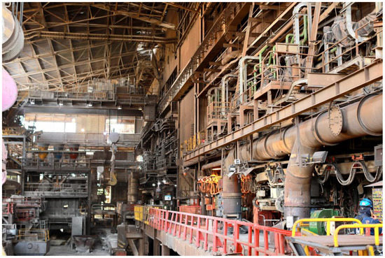
Figure 1.
Panoramic of the CMSA plant.
The main stage of ferronickel production is smelting. It is performed in the EAF. Figure 2 shows an inside view of the EAF, detailing its parts: (1) electrodes, (2) feeding tubes, (3) exhaust chimney, (4) top roof, (5) back-side wall, (6) input calcine, (7) sidewall, (8) waffle coolers, (9) plate coolers, (10) smelted ferronickel, (11) slag and (12) bottom hearth furnace lining. This study is focused on the temperature monitoring and forecasting of the side-wall; in particular, this temperature is measured by a thermocouples’ sensor network located at the plate coolers of the side-wall.
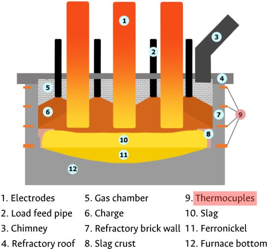
Figure 2.
Electric arc furnace components description.
2.2. Multivariate Time Series Forecasting
The multivariate time series forecasting process seeks the behavior of a set of output variables at a specific future time. Several methods have been developed to model the relationships between fluctuating variables in time series data. These methods can be divided into classical and machine learning methods. Among the classical methods are Autoregressive Integrated Moving Average (ARIMA), Vector Autoregression (VAR) and Vector Autoregression Moving-Average (VARMA) [27]. In contrast to classical methods, machine learning methods are effective in more complex time series prediction problems with multiple input variables, complex nonlinear relationships and missing data [28]. Some machine learning algorithms used for regression tasks have been used for time series forecasting; among them are Support Vector Regression, Random Forest, Extreme Gradient Boosting and Artificial Neural Networks [21]. Recently, deep learning advances have emerged as a satisfactory method to perform time series forecasting. The recurrent neural networks and their variants, such as Gated Recurrent Unit (GRU) and Long Short-Term Memory (LSTM), have addressed the problem of vanishing gradient and long-term dependencies, achieving remarkable behaviors [19].
2.3. Encoder–Decoder
For each time step in the LSTM and GRU models, each input corresponds to one of the outputs. In some cases, the objective is to predict an output given a different-length input, without correspondence; the models developed for these cases are known as seq-to-seq models. A typical model has two parts, an encoder and a decoder, with two different networks combined into one network; this network can take an input sequence and generate the next most probable sequence as the output. First, the encoder traverses the input at each time step to encode the complete sequence in a vector called the context vector; this vector acts as the last hidden state of the encoder and as the first hidden state for the decoder. This will contain information about all the input elements, which will help in the realization of the predictions [29].
2.4. Attention Mechanism
One of the frontiers in deep learning is attention mechanisms, which represent an evolution of encoder–decoder models, which were developed to improve the performance of long input sequences. In attention mechanisms, the decoder can selectively access the encoded information and uses a new concept for the context vector
, which is now calculated at each time step of the decoder, from the previous hidden state and all the hidden states of the encoder [29]. Trainable weights will be assigned to these states and produce different degrees of importance to all the elements in the input sequence. Special attention is paid to the most significant inputs—hence, they are named attention mechanisms [30]. The construction of the context vector starts from the combination of each time step j of the encoder with each time step t of the decoder. This expression is called the alignment score, and it is calculated as follows:
The terms , and correspond to the trainable weights mentioned above, where defines the function to calculate the alignment score, are associated with the hidden states of the encoder and with the hidden states of the decoder. The score must be normalized for each time step t; therefore, the SoftMax function is used together with the time steps j, and we obtain the attention weights , defined as follows:
This weight can capture the importance of the input at time step j to adequately decode the output at time step t. Finally, the context vector is found from the weighted sum of the relationship between all the encoder hidden values and attention weights:
The context vector allows more attention to the relevant inputs in the electric arc furnace variables. The term passed through the decoder and the probability for the next possible output is calculated. This operation applies to all time steps at the input. Then, the current hidden state is calculated, taking as input the context vector , the previous hidden state and the output from the previous time step:
Therefore, using this attention mechanism, the model can find the correlations between the different parts of the input sequence to the corresponding parts of the output sequence. For each time step, the decoder output is calculated by applying the “SoftMax” function to the hidden state [31].
2.5. Root Mean Squared Error (RMSE)
The performance of the multivariate time series forecasting deep learning model is calculated using the Root Mean Squared Error (RMSE):
where B is the number of data points in the time series to be estimated, is the actual value of the time series, and is the estimated value at the time i by the prediction model.
3. Dataset for Validation
Data used to train and validate the attention-based deep RNN model were obtained from a thermocouple sensor network located at the side-wall of an EAF in CMSA. Photography of the EAF side-wall is shown in Figure 3. The EAF side-wall is composed of 72 radially distributed panels. Figure 3 details a portion of the side-wall of 1 panel. The illustrated hoses carry water, which is used to cool the refractory walls of the EAF through the plate coolers (4 for each panel) and the waffle cooler (1 for each panel).
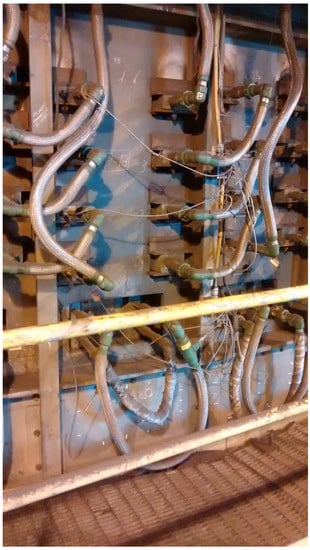
Figure 3.
Photography of CMSA furnace outside wall with its coolers.
The dataset used for model training and validation is composed of data recorded during 5 years, with 177,312 instances and 49 attributes, from an EAF located in Cerro Matoso, South 32 company. Data were collected every 15 min during a period of 1847 days, from September 9th of 2016 to September 30th of 2021. The input variables in the model were related to electrode current, voltage, arc, power, calcine feed, the chemical composition of the calcine, relative electrode position and 16 thermocouples. These 16 thermocouples were also taken as output variables to predict. In particular, 4 panels radially distributed 90 degrees in each quadrant of the furnace were selected to study the behavior of their plate cooler thermocouples. Each of the selected 4 panels had 4 plate coolers; thus, a total of 16 plate coolers were analyzed. The behavior of the time series of some of these variables in a time window that allows the trend to be seen can be observed in Figure 4.
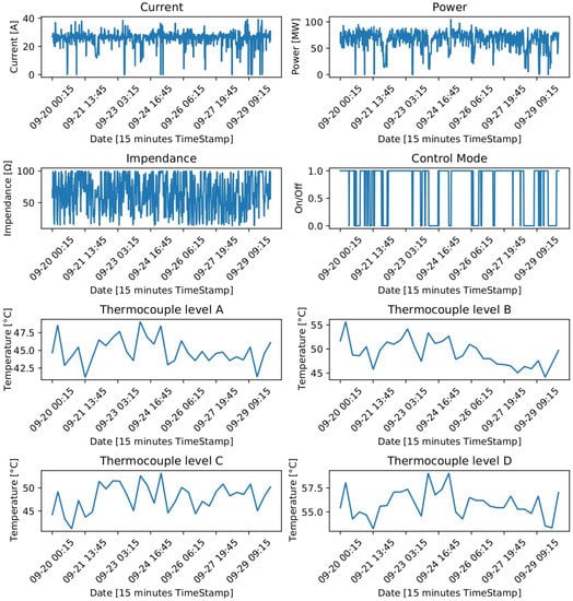
Figure 4.
Time series plot of some input and output variables in the dataset.
Several data preprocessing steps were performed to detect abnormal behavior in the used variables. These data preprocessing steps are listed below [32]:
- Remove duplicates;
- Treat empty and null values;
- Treat unique values;
- Encode strings;
- Remove negative temperatures;
- Eliminate variables with high variance;
- Remove variables with zero variance.
After verifying the data preprocessing, it was concluded that the 49 variables used to train and test the models did not present abnormal behaviors.
4. Multivariate Time Series Temperature Forecasting Model
The development of the multivariate time series temperature forecasting model comprised several stages. It started with the definition of the initial set of data already preprocessed, where the input variables for the models were selected as well as the variables to be predicted, the data were normalized so that the neural networks could work with them, the forecast time was defined and, in this way, the batch set generator was created for model training, as well as the data sequences for validation. The neural network models GRU and LSTM are designed to be incorporated with the attention mechanisms, and the RMSE loss function is defined with a warm-up period of 50 steps, which was not considered for the calculation of the evaluation metric, so we proceeded to train the model, validate it and generate the predictions to be able to compare them with the real values and make conclusions; this process is summarized in Figure 5.
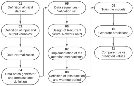
Figure 5.
Step by step development of the temperature prediction model.
The different layers that compose the multivariate time series deep learning attention models are summarized in Figure 6. Details of the shape and the number of parameters and connections of the layers in the multivariate time series deep learning attention model are noted. For the the gradient descent method, we used Adam optimization; this is a stochastic gradient descent (SGD) method that is based on adaptive estimation.
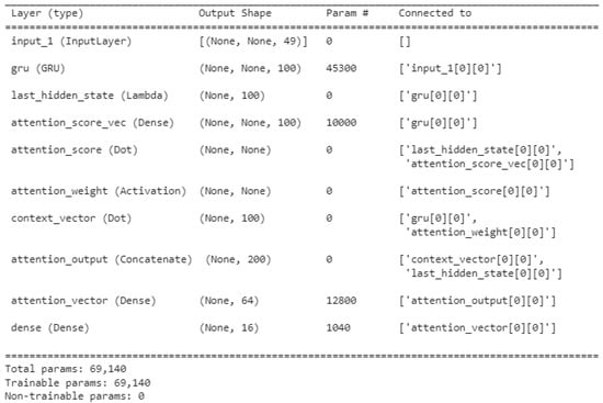
Figure 6.
Details of the shape and layer connections in the attention-based multivariate time series forecasting model.
5. Results and Discussion
Four deep neural network configurations corresponding to a GRU model and an LSTM model, with and without attention mechanisms, were designed, trained and tested, using 49 input variables to predict the 16 output variables corresponding to the thermocouple temperature. The Average Root Mean Square Error (RMSE) of these 16 output variables was used as a performance metric for each of the models.
5.1. Influence of Changing the Prediction Time
To determine the models’ behavior relating to the time interval under which they performed the prediction, the test was performed in a time window of 1 to 6 h predicting in the future for each model, increased by 1 h, as shown in Table 1 and Figure 7. From Table 1, it is evident that the Average RMSE values in the test set are larger than the train values. This is caused by the large amount of data belonging to the train set (90%) compared to the data from the test set (10%).

Table 1.
Average RMSE results of the train and test sets for the four different deep learning models in 6 different times.
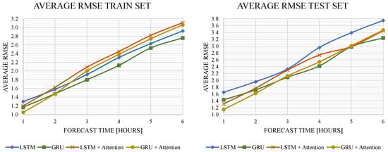
Figure 7.
Average RMSE behavior over the forecast time increases.
Figure 7 shows that the models with attention mechanisms had higher performance during a shorter prediction time. As the prediction time increased from 1 to 6 h, the models without attention mechanisms outperformed the other models. The GRU model obtained the best results with attention mechanisms for short times and without attention mechanisms for long times; for the short times, the longer input sequence in the GRU and LSTM networks resulted in worse prediction accuracy of the output sequence because it focused on all input variables equally. An attention mechanism can be used to alleviate this problem by focusing on more relevant input variables, since, as already described above, attention mechanisms can adaptively assign a different weight to each input sequence to automatically choose the most relevant features of the time series. Therefore, the model can effectively capture the long-term dependence on the time series.
As a result of the models evaluated in a 1 h forecast with and without attention, the predicted and true behaviors for a single thermocouple were compared, as shown in Figure 8. It is evident that the GRU model including attention (orange line) obtained a better representation of the true (green line) behavior. In contrast, the only GRU model (blue line) presented a more curly and distant behavior from the true data.
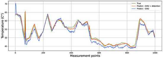
Figure 8.
Predictive versus true behavior of the GRU and GRU + attention models in the test set in one of the output thermocouples.
Additionally, in Table 2, the individual comparison of the RMSE error of each one of the thermocouples for each model used is presented. Here, it can be observed how some thermocouples have small prediction errors and others very large, which is averaged and leads to obtaining the Average RMSE of the total forecast.
Table 2.
RMSE results in the 16 thermocouples for the train and test sets versus the different deep learning models for a 6 h forecast.
5.2. Parameter Exploration
To evaluate the influence of some parameters in the Average RMSE results, an exploration procedure was executed. The changing of three different parameters was evaluated. These parameters were the optimizer, the number of cells in the GRU and LSTM models and finally the number of training epochs in the GRU model.
5.2.1. Changing of Optimizer
Four different optimizers were evaluated in order to compare their influence on the Average RMSE obtained by the GRU model. The four compared optimizers were RMSprop, Adam, Adamax and Nadam. As shown in Table 3, the best optimizer was Adam, obtaining an RMSE value in the train set of 3.01.
Table 3.
Average RMSE for GRU model with attention mechanisms against optimizer variance.
5.2.2. Change of GRU Cell Number
The variation in the number of GRU cells was studied by changing this number from 50 to 175, as shown in Table 4. The results indicate that, as the number of cells increases, the RMSE in the training set decreases, which does not mean that it is a good result because, in this way, the model is over-fitting with the training data, which means that, as the number of cells increases, the RMSE of the test set becomes worse because the model is so adjusted to the training data that when new and unknown data arrive in the model input, it is more difficult to make an adequate prediction.
Table 4.
Average RMSE for GRU model with attention mechanisms against GRU unit variance.
5.2.3. Change of LSTM Cell Number
Three different cell numbers were compared in the LSTM model. In this case, they were 32, 64 and 96, as shown in Table 5. The results show favorable behavior for the variation of 64 cells; as in the GRU model, more units does not lead to better results, due again to phenomena such as over-fitting.
Table 5.
Average RMSE for LSTM model with attention mechanisms against LSTM unit variance.
5.2.4. Changing of the Loss Behavior of the GRU Model through the Epochs
Figure 9 shows the loss behavior as the number of training epochs increases. From the results, it is evident that the first seven epochs are crucial in the decrease in loss, while, from epoch 7 onwards, the decrease in loss is scarce.
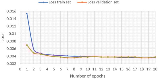
Figure 9.
Evaluation of the loss behavior of the GRU model through the epochs in the train set and test set.
5.3. Time Series Cross-Validation
Different cross-validation procedures have been developed to evaluate the behavior of a time series forecasting model [33]. In this study, three different approaches to perform time series cross-validation were used. These three approaches were (a) 7-fold moving origin, (b) Blocking Time Series Split and (c) Blocking Time Series Split with a static test set. Below, these three approaches are described and discussed.
5.3.1. Seven-Fold Moving Origin Time Series Split Cross-Validation
The first approach for the time series cross-validation was the 7-fold moving origin. This procedure involves cumulative training data from 1 October of 2020 to 1 September of 2021. Figure 10 illustrates the results at the top and details the data division in the bottom section. Seven different folds were evaluated; the first is the least in the training set, and as the folds increase, the size of the training data also increases. The size of the test set remains constant in each fold. The size of this test set is 4000 data instances.
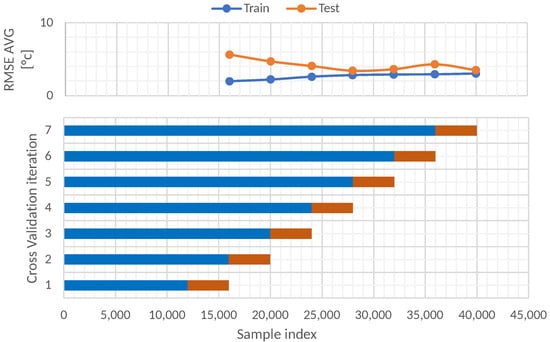
Figure 10.
Time series split cross-validation data partitions.
Table 6 shows the RMSE results for the train and test sets in each fold. As can be seen, the train RMSE increases as the number of folds increases. The opposite happens with the behavior of the RMSE test set; this indicates that it is better to train with numerous data because, with more data, the model can learn different scenarios that are presented in the furnace.
Table 6.
Average RMSE for training and test sets at each iteration with time series split.
5.3.2. Blocking Time Series Split
A second study using a blocking time series split cross-validation was performed. This validation approach consists of setting a fixed size of the train and test sets and moving across the entire dataset in several folds. In this case, 11 folds were used, and the train test had a size of 36,000 instances, whereas the test size had a size of 4000 instances. The shift between each fold was 140 days. Figure 11 illustrates the 11 folds and every train set in blue and test set in orange. In total, 177,312 instances of the dataset were used; these data began on 9th September of 2016 and ended on 30th September of 2021.
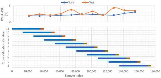
Figure 11.
Blocking time series split cross-validation data partitions.
The results after performing the 11-fold blocking time series split cross-validation are shown in Table 7. From these results, it is evident that the best results of RMSE in the train set (1.89) and test set (1.96) were reached by the oldest fold—in this case, the 11th fold. Furthermore, a decreasing behavior of the RMSE through the folds is evident for the train set. In contrast, the behavior of the test set is oscillatory decreasing. Considering the 11 folds, the average RMSE was 2.24 for the train set and 2.89 for the test set.
Table 7.
Average RMSE for training and test sets at each iteration with blocking time series split.
5.3.3. Blocking Time Series Split with Static Test Set
The last study for the time series cross-validation model was the blocking time series split with the static test set. In this case, 11 folds were also evaluated, but the test set remained the same for every fold. This test set was created with the most recent 4000 instances. Different training sets were tested. The shift between each training fold was 140 days. The size of each training set was 36,000 instances. Figure 12 illustrates the blocking time series split with static test set approach.
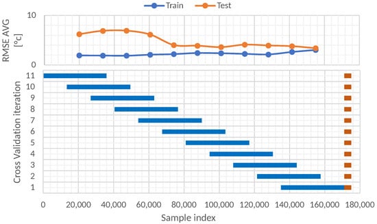
Figure 12.
Blocking time series split with static test set cross-validation data partitions.
The RMSE results of the blocking time series split with static test set approach are shown in Table 8. The results indicate that it is preferable to perform training with recent data since the RMSE increases as the training data move away from the test data. The RMSE in the test set changes from 3.37 for the first fold to 6.21 in the 11th fold, which represents an increase of 84.27%. Therefore, it is advisable to train the model every certain period to avoid obvious increases in the RMSE.
Table 8.
Average RMSE for training and test sets at each iteration, with blocking time series split with static test set.
5.4. Variable Importance Study
A study of the selected variables used to train and test the GRU model was performed to evaluate their influence on the RMSE values. This study was performed with the data of the 7th fold in the time series split cross-validation data partitions shown in Figure 10. Therefore, 36,000 instances composed the training set, whereas 4000 instances constituted the test set. Seven different scenarios were selected to train and test, removing the original number of variables as follows: (a) only with the 16 thermocouples to predict, (b) without furnace and electrode electric power, (c) without an electric arc, (d) without electrode position, (e) without electrode voltage, (f) without electrode current, (g) without the automatic control of electric power in the furnace (SAEE) mode, (h) without calcine chemistry and (i) using all 49 variables. The results of the RMSE comparison are shown in the bar chart of Figure 13. From the results in the bar chart, one can observe the difference between the RMSE results in the train and test sets, the latter being the one with the largest RMSE values. In particular, the worst results in the test set were obtained by the (i) all variables’ configuration, causing the error to reach the highest value of 3.45 in the test set. Consequently, when removing different groups of variables, the RMSE value improved. The lowest RMSE value of the test set of 3.22 was reached when the group (c) without electric arc was removed. Thus, it is better to remove the group of variables (c) related to the electric arc to develop the GRU model.
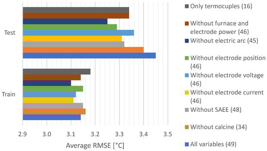
Figure 13.
Variable influence in the Average RMSE of the GRU model.
5.5. Study of Increasing the Number of Predicted Thermocouples to 76
Based on a request made by the CMSA engineering team in which they preferred to concentrate on the monitoring of the plate coolers in the lower row, the number of thermocouples to be monitored and predicted was increased. A study of the increase in the number of thermocouples was carried out, progressively evaluating their impact on the Average RMSE of the predictions.
The number of thermocouples was progressively increased from 16 until reaching 76 thermocouples. The RMSE values of the training set and the test set were measured for each increase; these values are shown in Table 9. It can be seen that the relationship between the increase in thermocouples and the Average RMSE of the predictions is directly proportional since, in Figure 14, the increasing trend of this evaluation metric can be observed due to the increase in the number of variables to be predicted.
Table 9.
Average RMSE results when increasing the number of thermocouples to predict in the GRU attention model.
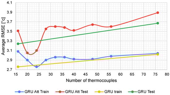
Figure 14.
Average RMSE behavior when increasing the output thermocouples to predict.
The increase that occurs in the Average RMSE is small compared with the increase in the number of thermocouples. There was an increase of 4.75 times in the number of thermocouples, while the RMSE in the training set remained approximately constant because there was more information that the model could use to obtain better relationships between the variables. On the other hand, for the test set, the RMSE increased only 1.1 times; this is because the number of variables and data that the model must predict is greater, but it is still a good prediction result.
From the results depicted in Figure 14, it can be seen that the attention GRU model improved the RMSE value when 24 thermocouples were predicted. Therefore, for a few thermocouples, the attention GRU model is better, whereas, for numerous thermocouples, it is recommended to use the GRU model without the attention mechanism.
5.6. Root Mean Squared Error Distribution by Each Thermocouple in the Test Set
Figure 15 illustrates the boxplot of the RMSE obtained by each thermocouple in the test set. In particular, the four quadrants of the furnace are separated. These quadrants are named as follows: northwest (section 18), southwest (section 19), southeast (section 20) and northeast (section 21). From the results, the southeast quadrant presents the lower error, while the southwest quadrant presents the highest. In general, the mean value of RMSE for each thermocouple is near to 0.4, reaching a maximum value of 1.75.
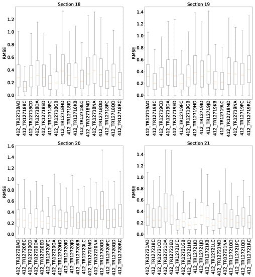
Figure 15.
Absolute error analysis by each thermocouple in the test set.
6. Conclusions
This work has shown the development of a multivariate time series deep learning model to predict the temperature behavior of a lining furnace. The developed model is based on an attention mechanism in the encoder–decoder approach of a recurrent neural network. The validation of the model was performed using data acquired in an industrial ferronickel furnace over a period of 5 years. The model considered the historical behavior of 49 variables involved in ferronickel production. Among these variables were the electrode current, voltage, power and position, besides the electric arc, the chemical composition and the temperature measured by the thermocouples themselves. These results were validated by a study carried out in terms of the Average RMSE calculated in 76 different thermocouples located in the furnace lining side-wall at four different heights.
The principal conclusions of this work are as follows:
- The temperature of the lining furnace at different heights of the wall and in different sectors was satisfactorily predicted using the developed deep learning model.
- The results showed that the prediction time influenced the obtained Average RMSE, which was better when predicted in a time window of 1 h in the future when the attention mechanism was used. RMSE values increased as the time window increased.
- A comparison between four different approaches using GRU, LSTM, and their attention-based variants was performed. The best RMSE results were obtained using the GRU attention-based model.
- Three different time series cross-validation procedures were used: the 7-fold moving origin time series split, the Blocking Time Series Split and the Blocking Time Series Split with static test set. The results showed that, over time, the model lost its ability to correctly predict temperatures. Therefore, it is recommended to retrain the model every year to maintain an RMSE value of around 4 °C.
- A study increasing the number of thermocouples to predict from 16 to 76 was carried out. The results showed that the Average RMSE was maintained at a value near to 4 °C, which is allowed in the furnace operation due to the normal operation conditions.
As general conclusions, we can highlight that this work aimed to provide and validate a forecast temperature methodology that is applied to an electric arc furnace. The validation was performed by using real data from a furnace of the Cerro Matoso S.A. and results were validated by staff from the same company. Although the methodology was implemented in this furnace, the paper presents the steps to apply it to any multivariable process to predict the behavior of a variable.
As future works, the following ideas will be explored:
- An online learning-based stream data approach will be developed to evaluate damages in the refractory walls using the developed model. Moreover, the concept of drift detection and treatment in these variables will be studied.
- The methodology will be adapted to forecast other important variables in this furnace, such as the thickness of the refractory wall by predicting, among others, the flow heat in these walls. Since thickness can be measured directly by the operational conditions, it can be obtained by a model that uses forecasted variables.
Author Contributions
All authors contributed to the development of this work; their specific contributions are as follows: conceptualization, D.A.T., C.P., B.R., J.R. and W.V.; data organization and preprocessing, D.F.G.-R., J.X.L.-M., D.A.T. and F.P.; methodology, J.X.L.-M., D.F.G.-R., D.A.T. and C.P.; validation, J.X.L.-M., D.A.T., C.P., F.P., W.V., J.R. and B.R. All authors have read and agreed to the published version of the manuscript.
Funding
This work has been funded by the Colombian Ministry of Science through grant number 786, “Convocatoria para el registro de proyectos que aspiran a obtener beneficios tributarios por inversión en CTeI”. This work has been partially funded by the Spanish Agencia Estatal de Investigación (AEI)—Ministerio de Economía, Industria y Competitividad (MINECO), and the Fondo Europeo de Desarrollo Regional (FEDER) through the research project DPI2017-82930-C2-1-R, and by the Generalitat de Catalunya through the research project 2017-SGR-388.
Institutional Review Board Statement
Not applicable.
Informed Consent Statement
Not applicable.
Data Availability Statement
Not applicable.
Acknowledgments
The authors express their gratitude to Luis Bonilla for providing the dataset and some very useful information about the furnace operation. In the same manner, we thank Janneth Ruiz, Cindy Lopez and Carlos Galeano Urueña for their support throughout the development of this work.
Conflicts of Interest
The authors declare no conflict of interest.
Abbreviations
The following abbreviations are used in this manuscript:
| RMSE | Root mean square error |
| RNN | Recurrent neural network |
| LSTM | Long short-term memory |
| GRU | Gated recurrent unit |
| SHM | Structural health monitoring |
| EAF | Electric arc furnace |
| CNN | Convolutional neural network |
| CMSA | Cerro Matoso S.A. |
References
- Anaya, M. Design and Validation of a Structural Health Monitoring System Based on Bio-Inspired Algorithms. Ph.D. Thesis, Universitat Politècnica de Catalunya, Barcelona, Spain, 2016. [Google Scholar]
- Tibaduiza Burgos, D.A.; Gomez Vargas, R.C.; Pedraza, C.; Agis, D.; Pozo, F. Damage Identification in Structural Health Monitoring: A Brief Review from its Implementation to the Use of Data-Driven Applications. Sensors 2020, 20, 733. [Google Scholar] [CrossRef] [Green Version]
- Diamanti, K.; Soutis, C. Structural health monitoring techniques for aircraft composite structures. Prog. Aerosp. Sci. 2010, 46, 342–352. [Google Scholar] [CrossRef]
- Tibaduiza, D. Design and Validation of a Structural Health Monitoring System for Aeronautical Structures. Ph.D. Thesis, Universitat Politècnica de Catalunya, Barcelona, Spain, 2013. [Google Scholar]
- Senyurek, V. Detection of cuts and impact damage at the aircraft wing slat by using Lamb wave method. Measurement 2015, 67, 10–23. [Google Scholar] [CrossRef]
- Rytter, A. Vibrational Based Inspection of Civil Engineering Structures. Ph.D. Thesis, Department of Building Technology and Structural Engineering, Aalborg University, Aalborg, Denmark, 1993. [Google Scholar]
- Kaloop, M.R.; Hu, J.W. Damage Identification and Performance Assessment of Regular and Irregular Buildings Using Wavelet Transform Energy. Adv. Mater. Sci. Eng. 2016, 2016, 11. [Google Scholar] [CrossRef] [Green Version]
- Yamamoto, K.; Miyamoto, R.; Takahashi, Y.; Okada, Y. Experimental Study about the Applicability of Traffic-induced Vibration for Bridge Monitoring. Eng. Lett. 2018, 26, 276–280. [Google Scholar]
- Fan, X.P.; Lu, D.G. Reliability prediction of bridges based on monitored data and Bayesian dynamic models. In Key Engineering Materials; Trans Tech Publ.: Freienbach, Switzerland, 2014; Volume 574, pp. 77–84. [Google Scholar]
- Endsley, A.; Brooks, C.; Harris, D.; Ahlborn, T.; Vaghefi, K. Decision support system for integrating remote sensing in bridge condition assessment and preservation. In Sensors and Smart Structures Technologies for Civil, Mechanical, and Aerospace Systems 2012; International Society for Optics and Photonics: San Diego, CA, USA, 2012; Volume 8345, p. 834548. [Google Scholar]
- Tibaduiza, D.A.; Leon-Medina, J.X.; Gomez, R.; Ricardo, J.; Rueda, B.; Zurita, O.; Forero, J.C. Structural Health Monitoring System for Furnace Refractory Wall Thickness Measurements at Cerro Matoso SA. In European Workshop on Structural Health Monitoring; Rizzo, P., Milazzo, A., Eds.; Springer International Publishing: Cham, Switzerland, 2021; pp. 414–423. [Google Scholar]
- Voermann, N.; Gerritsen, T.; Candy, I.; Stober, F.; Matyas, A. Furnace technology for ferro-nickel production-an update. In Proceedings of the International Laterite Nickel Symposium, Charlotte, NC, USA, 14–18 March 2004. [Google Scholar]
- Jiao, K.; Zhang, J.; Hou, Q.; Liu, Z.; Wang, G. Analysis of the relationship between productivity and hearth wall temperature of a commercial blast furnace and model prediction. Steel Res. Int. 2017, 88, 1600475. [Google Scholar] [CrossRef]
- Leon-Medina, J.X.; Camacho-Olarte, J.; Rueda, B.; Vargas, W.; Bonilla, L.; Ruiz, J.; Sofrony, J.; Guerra-Gomez, J.A.; Restrepo-Calle, F.; Tibaduiza, D.A. Monitoring of the refractory lining in a shielded electric arc furnace: An online multitarget regression trees approach. Struct. Control. Health Monit. 2022, 29, e2885. [Google Scholar] [CrossRef]
- Klimas, M.; Grabowski, D. Application of Long Short-Term Memory Neural Networks for Electric Arc Furnace Modelling. In Intelligent Data Engineering and Automated Learning—IDEAL 2021; Yin, H., Camacho, D., Tino, P., Allmendinger, R., Tallón-Ballesteros, A.J., Tang, K., Cho, S.B., Novais, P., Nascimento, S., Eds.; Springer International Publishing: Cham, Switzerland, 2021; pp. 166–175. [Google Scholar]
- Leon-Medina, J.X.; Camacho, J.; Gutierrez-Osorio, C.; Salomón, J.E.; Rueda, B.; Vargas, W.; Sofrony, J.; Restrepo-Calle, F.; Pedraza, C.; Tibaduiza, D. Temperature Prediction Using Multivariate Time Series Deep Learning in the Lining of an Electric Arc Furnace for Ferronickel Production. Sensors 2021, 21, 6894. [Google Scholar] [CrossRef] [PubMed]
- McCoy, J.T.; Auret, L. Machine learning applications in minerals processing: A review. Miner. Eng. 2019, 132, 95–109. [Google Scholar] [CrossRef]
- Yang, Q.; Shen, D. Learning Damage Representations with Sequence-to-Sequence Models. Sensors 2022, 22, 452. [Google Scholar] [CrossRef] [PubMed]
- Leon-Medina, J.X.; Vargas, R.C.G.; Gutierrez-Osorio, C.; Jimenez, D.A.G.; Cardenas, D.A.V.; Torres, J.E.S.; Camacho-Olarte, J.; Rueda, B.; Vargas, W.; Esmeral, J.S.; et al. Deep Learning for the Prediction of Temperature Time Series in the Lining of an Electric Arc Furnace for Structural Health Monitoring at Cerro Matoso (CMSA). Eng. Proc. 2020, 2, 23. [Google Scholar]
- Dong, M.; Grumbach, L. A hybrid distribution feeder long-term load forecasting method based on sequence prediction. IEEE Trans. Smart Grid 2019, 11, 470–482. [Google Scholar] [CrossRef] [Green Version]
- Lim, B.; Zohren, S. Time-series forecasting with deep learning: A survey. Philos. Trans. R. Soc. A 2021, 379, 20200209. [Google Scholar] [CrossRef] [PubMed]
- Zhao, H.; Wang, Y.; Duan, J.; Huang, C.; Cao, D.; Tong, Y.; Xu, B.; Bai, J.; Tong, J.; Zhang, Q. Multivariate Time-series Anomaly Detection via Graph Attention Network. In Proceedings of the 2020 IEEE International Conference on Data Mining (ICDM), Sorrento, Italy, 17–20 November 2020. [Google Scholar]
- Barić, D.; Fumić, P.; Horvatić, D.; Lipic, T. Benchmarking attention-based interpretability of deep learning in multivariate time series predictions. Entropy 2021, 23, 143. [Google Scholar] [CrossRef] [PubMed]
- Gangopadhyay, T.; Tan, S.Y.; Jiang, Z.; Meng, R.; Sarkar, S. Spatiotemporal Attention for Multivariate Time Series Prediction and Interpretation. In Proceedings of the ICASSP 2021—2021 IEEE International Conference on Acoustics, Speech and Signal Processing (ICASSP), Toronto, ON, Canada, 6–11 June 2021. [Google Scholar]
- Janzen, J.; Gerritsen, T.; Voermann, N.; Veloza, E.; Delgado, R. Integrated furnace controls: Implementation on a covered-arc (shielded arc) furnace at cerro matoso. In Proceedings of the 10th International Ferroalloys Congress, Cape Town, South Africa, 1–4 February 2004; Volume 1, p. 4. [Google Scholar]
- Voermann, N.; Gerritsen, T.; Candy, I.; Stober, F.; Matyas, A. Developments in furnace technology for ferronickel production. In Proceedings of the 10th International Ferroalloys Congress, Cape Town, South Africa, 1–4 February 2004; p. 455. [Google Scholar]
- Mills, T.C. Applied Time Series Analysis: A Practical Guide to Modeling and Forecasting; Academic Press: Cambridge, MA, USA, 2019. [Google Scholar]
- Bontempi, G.; Ben Taieb, S.; Le Borgne, Y.A. Machine Learning Strategies for Time Series Forecasting. In Tutorial Lectures, Proceedings of the Business Intelligence: Second European Summer School, eBISS 2012, Brussels, Belgium, 15–21 July 2012; Aufaure, M.A., Zimányi, E., Eds.; Springer: Berlin/Heidelberg, Germany, 2013; pp. 62–77. [Google Scholar] [CrossRef]
- Du, S.; Li, T.; Yang, Y.; Horng, S.J. Multivariate time series forecasting via attention-based encoder–decoder framework. Neurocomputing 2020, 388, 269–279. [Google Scholar] [CrossRef]
- Luong, M.T.; Pham, H.; Manning, C.D. Effective approaches to attention-based neural machine translation. arXiv 2015, arXiv:1508.04025. [Google Scholar]
- Rémy, P. Keras Attention Mechanism. 2021. Available online: https://github.com/philipperemy/keras-attention-mechanism (accessed on 24 September 2021).
- Camacho-Olarte, J.; Torres, J.E.S.; Jimenez, D.A.G.; Medina, J.X.L.; Vargas, R.C.G.; Cardenas, D.A.V.; Gutierrez-Osorio, C.; Rueda, B.; Vargas, W.; Burgos, D.A.T.; et al. A Data Cleaning Approach for a Structural Health Monitoring System in a 75 MW Electric Arc Ferronickel Furnace. Eng. Proc. 2020, 2, 21. [Google Scholar] [CrossRef]
- Schnaubelt, M. A comparison of machine learning model validation schemes for non-stationary time series data. In Technical Report, FAU Discussion Papers in Economics, No. 11/2019; Friedrich-Alexander-Universität Erlangen-Nürnberg, Institute for Economics: Nürnberg, Germany, 2019. [Google Scholar]
Publisher’s Note: MDPI stays neutral with regard to jurisdictional claims in published maps and institutional affiliations. |
© 2022 by the authors. Licensee MDPI, Basel, Switzerland. This article is an open access article distributed under the terms and conditions of the Creative Commons Attribution (CC BY) license (https://creativecommons.org/licenses/by/4.0/).