Modeling and Verification of Asynchronous Systems Using Timed Integrated Model of Distributed Systems

Abstract

In modern computer systems, distributed systems play an increasingly important role, and modeling and verification are crucial in their development. The specificity of many systems requires taking this into account in real time, as time dependencies significantly affect the system’s behavior, when achieving the goals of its processes or with adverse phenomena such as deadlocks. The natural features of distributed systems include the asynchrony of actions and communication, the autonomy of nodes, and the locality of behavior, i.e., independence from any global or non-local features. Most modeling formalisms are derived from parallel centralized systems, in which the behavior of components depends on the global state or the simultaneous achievement of certain states by components. This approach is unrealistic for distributed systems. This article presents the formalism of a timed integrated model of distributed systems that supports all of the mentioned features. The formalism is based on the relation between the states of the distributed nodes and the messages of distributed computations, called agents. This relation creates system actions. A specification in this formalism can be translated into timed automata, the most popular formalism for specifying and verifying timed parallel systems. The translation rules ensure that the semantics of T-IMDS and timed automata are consistent, allowing use of the Uppaal validator for system verification. The development of general formulas for checking the deadlock freedom and termination efficiency allows for automated verification, without learning temporal logics and time-dependent formulas. An important and rare feature is the finding of partial deadlocks, because in a distributed system a common situation occurs in which some nodes/processes are deadlocked, while others work. Examples of checking timed distributed systems are included.

1. Introduction

The formalism of the distributed systems specification was developed at the Institute of Computer Science, Warsaw University of Technology. The formalism, called timed integrated model of distributed system (T-IMDS, based on the earlier timeless IMDS [1,2]) has a set of general features that distinguish it from other formalisms:

• timed specification and verification: distributed systems are asynchronous in nature, and time dependencies may substantially change their observed features; as in the Russian fairy tale: the crane offered the heron a marriage; the heron initially refused, but later changed her mind and offered to charm the crane when he took offense …; as a result, they see each other often, but each of them is proud and refuses when the latter is ready to propose; the tale has no end, because its characters act exactly in counter-phase, they do not synchronize in any way; in particular, some deadlocks can disappear due to time dependencies, while others can arise.
• communication duality: expressing the distributed system in terms of nodes with their states and agents with their messages, emphasizing communication duality in distributed systems: message passing versus resource sharing; the system specification can be switched between two system views: node view and agent view, yet with both in a uniform structure;
• locality: the node’s action is executed based on the current situation of the node (without any association with other nodes); no event outside the node (except for messages sent to it) can affect the behavior of the node;
• autonomy: each decision regarding the execution of the actions of the node (including the choice between many possible actions) is taken autonomously; the only way to influence the behavior of a node is to send a message to it (the message may enable an action that was previously disabled); no order is established in the set of pending messages, such as a stack or queue, the node autonomously decides which message will initiate the next action;
• asynchrony: the synchronization of nodes with agents is hidden inside processes (in actions belonging to processes); therefore, processes are perceived as asynchronous from the outside; also the communication channels are asynchronous: the message is sent irrespective of the local situation of the target node, in particular, whether it is waiting for this message or performing completely different operations;
• automated verification: expressing essential features of the distributed system’s behavior using general temporal formulas [2], not related to the internal structure of the system being verified.

A large selection of timed specification and verification techniques are offered; some are mentioned in Section 2. This is why we extended our IMDS formalism to cover real-time dependencies.

Locality and autonomy are obvious features of distributed systems. Asynchrony is very much needed between cooperating distributed nodes, because synchronous behavior requires some knowledge of the global state, which is difficult to obtain in a distributed system (or which cannot be obtained at all). Imagine a distributed component, for example a Büchi automaton [3] or Zielonka’s automaton [4]. If such an automaton is to communicate with another, both of them must follow a common transition. Obviously, such behavior is impossible: how would the automaton learn that they have both reached matching states or enabled matching transition? This principle breaks asynchrony (two automata cannot synchronize on states or transitions), locality (non-local/global information of the state of the other component is needed), and autonomy (the decision about the component behavior must depend only on its history and its preferences, rather than on the state of other components). Therefore, synchronous actions or other forms of direct synchronization are unrealistic in the description of distributed system behavior. Please note that such models are wrongly called distributed in numerous articles (e.g., [4]).

Communication duality is often emphasized as a theoretical feature of distributed systems, for example, in comparing client-server and remote procedure call (RPC) models, but rarely do both aspects occur in a uniform environment. In [5], they are both described, but as separate and opposite models. We argue that those models can simply be different points of view of a single, uniform system. The image of the modeled system depends on the manner of action grouping, rather than being a substantial property of the system itself.

Finally, identifying partial (sometimes called local) deadlocks and checking the distributed termination with model checking techniques [6] requires the designer to have some knowledge of temporal logic, since features should be expressed in terms of the elements of the particular system under verification [7,8]. The reason for this is that the deadlock is often identified as a global state, with no outgoing transitions [9]. Alternatively, a temporal formula that guarantees that the system is stuck in a deadlocked state is applied [10]. In both solutions, only a total deadlock can be identified. Other techniques are used for partial deadlock identification, but typically in systems having a required structure [11,12] (for example, looping systems). However, a situation in which some processes are deadlocked while other processes work is usual in distributed systems and should be found in systems of arbitrary shape.

The contribution of this article is the introduction of the timed integrated model of distributed systems (T-IMDS), which overcomes all the above-mentioned limitations in the specification and verification of distributed systems.

• The specification is real-time aware, which is not novel between formalisms, but is an important step in IMDS evolution.
• It is based on a relation between two pairs of a distributed node state and the distributed computation (called an agent) message. The input pair only triggers a system action and produces a new pair that simply waits for its occasion (the consecutive actions of the node and the agent need not even be enabled at this moment). This counters the requirements for synchrony and non-locality of actions. The description models asynchronous actions, in which nothing depends on the synchronous delivery of any items needed to fire the actions. Distributed components make their autonomous moves based only on their local elements, and they do not depend on any global or non-local features of the distributed system.
• Communication duality (client–server versus RPC) is incorporated in the model; the views are only the decompositions or cuts of the system, the given view is achieved by a specific grouping of the actions; however, the set of actions remains the same.
• Identification of partial deadlocks and the partial distributed termination, as well as total–general temporal formulas are defined for this purpose, related to the features of the formalism, rather than to the features of the given verified system. The developed verification algorithms (which are beyond the scope of this article) allow both timeless and timed verification. The compatibility with Uppaal timed automata allows for verification under the external verifier Uppaal [13,14].

The Dedan verification environment (deadlock analyzer) was developed based on IMDS. It offers:

• interface to the specifications of the distributed system, text or graphic,
• a simple built-in temporal verifier (based on the TempoRG verifier [15]) for checking models of small and medium systems,
• simulator,
• export to external verifiers: Spin [16] for LTL verification, NuSMV [17] for LTL/CTL verification, Uppaal for CTL/TCTL verification.

The behavior of a distributed system may be time-dependent, as system changes may take some time. As a result, the dependence between periods associated with individual system changes can influence deadlock situations. Timed Petri nets and timed automata (TA) are two of the most popular formalisms for expressing the behavior of time-limited systems (TA) [18,19,20]. While automata-based models, as well as IMDS, can be transformed to Petri nets [21], they are not so attractive in our opinion, because it is not easy to extract the processes from the specification. We use Petri nets for the structural analysis of a verified system and some kinds of model checking [22]. The temporal logic timed CTL (TCTL) is associated with TA [18,23]. Two types of transition: progress transitions and time transitions are introduced to describe system changes and the flow of time:

• Progress transition (or: transition): If the Boolean expression on the automaton’s transition is true, the progress transition (or transition) is executed. This expression is composed of integers and clock values. TA actions are symbols associated with transitions (not to be confused with IMDS actions, we will use the term symbol for TA actions). When two or more automata have the same action symbol, the transitions are synchronous. The transitions are otherwise executed in an interleaving way [24].
• Timed transition can be executed if all of the automata in the set have time invariants (relationships between clock values and integers) in their current locations. All the clocks are simultaneously shifted by the same value (not exceeding any invariant).

This article is organized as follows: Section 2 covers related work on timed varication formalisms, especially timed automata. Section 3 deals the basic timeless formalism: the integrated model of distributed systems, and verification rules in IMDS, which are the basis of extension to timed systems. Section 4 covers the Uppaal timed automata model, the target formalism to which timed IMDS is converted. The timed version of IMDS is described in Section 5. The formal translation of T-IMDS to UTA is presented in Section 6. Section 7 gives two examples of distributed timed systems and their verification in the Dedan/Uppaal environment. The work is concluded in Section 8. The Appendix A contains the proof of equivalence between the semantics of T-IMDS and its implementation in UTA.

2. Related Work: Timed Automata and Other Timed Formalisms

Since system changes may take time, the dependencies between durations associated with specific changes may play a role in deadlock situations. Timed Petri nets and timed automata [19,20,25,26] are two of the most prominent formalisms for expressing the behavior of time-limited systems. Other real-time modeling techniques include hybrid automata [27] and timed CSP [28]. For discrete time modeling, among others, DTG (durational transition graphs [29]) and EMLAN [30] are used.

Real-time CTL (RTCTL, having time constraints attributed to temporal operators [31,32]), quantitative CTL (QCTL, with unit-delay transitions [33]), timed CTL (TCTL, connected with timed automata [18]) and bounded real-time model checking [34] were also developed. Discrete-time model checking example formalisms include clocked CTL (CCTL, based on time intervals in discrete-time systems [35]) and discrete-time CTL (DTCTL for embedded systems [30]).

Timed automata (TA [18]) are related to Büchi automata [3], but with the addition of time constraints. Automata execute their transitions separately (in an interleaving manner [36]), except for transitions on shared symbols, which synchronize the automata. A set of real-time clocks is used to achieve time limitations. The clocks are variables, with values ranging in ℝ_≥0, multiples of a basic unit of time (a unit in short). A clock value is a real number, yet we can watch it while its values are integers or between integers. For example, with two clocks, x and y, we can examine the system in a circumstance where x is 2 and y is between 0 and 1. Similarly visible is the relationship between clocks (as x < y or x < y + 1). Time limitations, which determine the values of clocks at which specific transitions may be fired (for example, x ≥ 1), are attributed to the transitions of timed automata. Time invariants can also be enforced on automata states (called locations in TA). The time invariant expresses, in terms of clock values, how long an automaton may stay in a given location, such as y < 3. On transition, the clocks may be reset.

The TA transitions are instantaneous; the clocks advance while the automata remain in their locations. As a result, there are two sorts of advancement in TA: executing progress transitions and passing of time, referred to as timed transitions. The articles [18,23] give a complete overview of timed automata and their semantics.

Compound progress transitions and compound timed transitions are used to define the semantics of a set of timed automata:

• If a Boolean expression on a progress transition (or simply: transition, also termed action transition [37]) outgoing from a current location of a timed automaton TA is fulfilled, the transition can be executed. This expression is made up of integer constants and clocks. A difference is only allowed when two clocks are utilized in the expression. If more than one transition (in the same automaton or different automata) can be executed in a set of TA, the choice is nondeterministic. Transitions are denoted by symbols known as actions (do not confuse with IMDS actions, we use the term symbol for TA action). When two or more automata have the same action symbol, the transitions are executed synchronously. Otherwise, the transitions interleave.
• The timed transition can be executed if all of the automata in the set have their time invariants fulfilled in their current locations. The execution is based on synchronously advancing all clocks (by the same, real value > 0). The smallest difference between the maximum value of a clock used in an invariant and the present value used in this invariant is the maximum value to which the clocks can be advanced. If the invariants x < 2 and y ≤ 3 are present, and the current clock values are x = 1.5 and y = 2.6, the highest value is 0.4, which advances x to 1.9 and y to 3.

The option is nondeterministic if both a progress and a timed transition are enabled. It is important to note that there may be an endless number of timed transitions if a timed transition is possible. If a timed transition of 1 unit is achievable, perhaps a transition of 0.9 units makes no difference. As a result, timed regions (equivalence classes) are introduced to the formalism, with integer limits. The greatest integer relative to the clock is the maximum value used. Given integer parts of all clocks and an equal sign of the fractional part of clock differences (0 is treated as a distinct, third sign), a region, such as ⎣x⎦ = 1, ⎣y⎦ = 2, (x − ⎣x⎦) − (y − ⎣y⎦) > 0, is obtained. This rule generates a set of clock regions. Above their maximum values, the relations between the clocks are not examined.

Since infinitely many time transitions between a pair or regions are possible, a region succession graph is created.

2.1. Timed Automaton-Syntax

Here, we give the definition of timed automata, a base of Uppaal extension. A timed automaton TA is a tuple (L, l₀, Z, Q, E, J_l) where:

• L = {l₀, l₁, …} is a finite set of locations,
• l₀ ∈ L is an initial location,
• Z = {c₀, c₁, …} is the set of clocks,
• Q denotes a set of labels (interpreted as actions on transitions, do not confuse with IMDS actions),
• every location l ∈ L is mapped by J_l(l) to a set of valuations of clocks in Z, over a Cartesian product of ${ℝ}_{\ge 0}^Z$, for example, J_l(l) = {c₁-c₂ > 2},
• E ⊆ L × Q × J_ll × 2^Z × L—set of transitions: e = (l, q, J_ll(l,l′), r, l′) ∈ E
  • J_ll is a set of functions for pairs l,l′ ∈ L, every transition (l,l′), is mapped by J_ll(l,l′) to a set of valuations of clocks in Z over a Cartesian product of ${ℝ}_{\ge 0}^Z$, just as J_l(l) for a location l,
  • r ∈ 2^Z indicates a subset of clocks in Z that are reset on transition.

2.2. Timed Automaton-Semantics

The semantics of a TA is:

Let (L, l₀, Z, Q, E, J_l) be an TA.

The semantics is defined as an LTS—labeled transition system ⟨Vertices, vertex₀, ▶⟩, where:

• Vertices ⊆ L × ${ℝ}_{\ge 0}^Z$ is the set of LTS vertices for the automaton TA (because the term state is reserved for IMDS node states, we use the term vertex instead),
• vertex₀ = (l₀, u₀) ∈ Vertices is the initial vertex, u₀ maps all clocks c ∈ Z to 0.
• ▶ = ▶_t ∪ ▶_p is the transition relation such that:
  • (l, u) ▶_t (l, u + d) if ∀d′: 0 ≤ d′ ≤ d ⇒ u + d′ ∈ J_l(l) – timed transition,
  • (l, u) ▶_p (l′, u′) if there exists e = (l, q, J_ll(l,l′), r, l′) ∈ E

Such that u ∈ J_ll(l,l′); u′ = [r ↳ 0]u – progress transition;

where

for d′ ∈ ${ℝ}_{\ge 0}^Z$, u + d′ maps each clock c in Z to the value u(c) + d′,

[r ↳ 0]u, r ⊂ Z, denotes the clock valuation, which maps each clock in r to 0 and agrees with u over Z\r.

2.3. Network of TA

NTA is a network of timed automata over a common set of clocks and labels (actions). NTA is itself a TA, it is constructed in the following way:

NTA = (L, l⁰, Z, Q, E, J_l) consists of n TA, TA_i = (L_i, l_i⁰, Z_i, Q_i, E_i, J_li) with i = 1, …, n. The individual elements of NTA are:

• A set of locations is a Cartesian product L = L₁ × … × L_n, l ∈ L is a location vector l = (l₁, …, l_n), l_i ∈ L_i.
• l⁰ ∈ L is an initial location vector l⁰ = (l₁⁰, …, l_n⁰), l_i⁰ ∈ L_i.
• Z is a common set of clocks—a union of sets of clocks Z = Z₁ ∪ … ∪ Z_n.
• Q is a common set of labels—symbols on transitions Q = Q₁ ∪ … ∪ Q_n.
• Location invariant functions are composed into a common function over location vectors J_l(l) = J_l1(l₁) ∧ … ∧ J_ln(l_n).

2.4. The Semantics of the Network of TA

Let TA_i = (L, l⁰, Z, Q, E, J_l).

Let l⁰ = (l₁⁰, …, l_n⁰) be the initial location vector.

l[l_i/l_i′] denotes the location vector where l_i′ replaces the i^th element l_i of L.

The semantics of a network on n TA is defined as an LTS ⟨Vertices, vertex₀, ▶⟩, where:

• Vertices = (L₁ × … × L_n) × ${ℝ}_{\ge 0}^Z$ is the set of global LTS vertices,
• vertex₀ = (l₀; u₀) ∈Vertices is the initial vertex, u₀ maps all clocks c ∈ Z to 0,
• ▶ = ▶_t ∪ ▶_p is the transition relation defined by:

  -

  (l, u) ▶_t (l, u + d) if ∀_d′ 0 ≤ d′ ≤ d ⇒ u + d′ ∈ J_l(l)—timed transition,

  -

  if there exists a symbol q ∈ Q, for which there exist transitions e_i, e_j, … in TA_i, TA_j, … (at least one, but if more, then in distinct automata): e_i = (l_1i, q, J_lli(l_1i,l_2i), r_i, l_2i) ∈ E_i, e_j = (l_1j, q, J_llj(l_1j,l_2j), r_j, l_2j) ∈ E_j, …then there exists the transition e = (l₁, q, J_ll(l₁,l₂), r, l₂) ∈ ▶_p such thatu ∈ J_ll(l[l_1i/l_2i, l_1j/l_2j, …]), u′ = [r_i ∪ r_j ∪ …↳ 0]u—progress transition, Comment: There is a synchronization transition if more than one transition in distinct TA have the same q label on their transitions.

2.5. The Uppaal Extesion to TA

Transitions are executed simultaneously by the original TA if they are triggered by shared symbols (which enable transitions). A common symbol can synchronize more than two automata. However, standard TA are useless, because they do not apply urgent channels (a timed transition can be executed while a progress transition is enabled) and the do not use variables; thus, no value can be passed between automata that explode the automata layout. Therefore, we give the definition of Uppal timed automata (UTA [13]) in Section 4.

Communication channels replace the common symbols that trigger transitions in Uppaal timed automata. Sending and receiving a signal synchronously via channels is accomplished by utilizing a shared channel symbol and two characters indicating sending and receiving, ! and ?, respectively, as in chan! and chan? As it specifies the communication direction, this method better reflects distributed systems. Broadcast communication entails multiple automata receiving a signal given by one automaton.

The channel can be labeled urgent, in which case transitions are enabled, with common channel symbols enabling these transitions: chan! and chan?, taking precedence over time flow in locations, preventing communication over an urgent channel from being delayed. However, in IMDS, using such a technique eliminates communication asynchrony. As a result, asynchronous communication requires the introduction of asynchronous channels.

3. Integrated Model of Distributed Systems (IMDS)

The most straightforward description of IMDS is as follows: there are distributed nodes in the system, which are characterized by their current states and agents conducting distributed calculations, the progress of which is determined by their current messages directed to individual nodes. If the message matches the node state, an action is fired (invoked) that consumes the message and state and provides the node’s next state and the agent’s next message. Therefore, actions are the relationship between pairs (message, state), input and output ones; that is all. However, a more detailed definition should be introduced to define processes in the system and verify the system.

An IMDS system [2] consists of a set of nodes, each represented by its current state as a pair: (node, value). Each node offers services that distinguish different calls to the same node. The set of agents represents distributed computing. In the context of agents, messages are created that invoke node services. The message is a triple: (agent, node, service). States and messages are, together, called elements. They change their roles as process carriers and means of communication in dual views of distributed systems.

The actionrefers to how the service is carried out (on the node designated by the message). The action switches the node’s current state to the next one and sends the next agent message. This new message might be sent to the same or a different node. Distributed computation is carried out as a series of actions that alter the states of the nodes involved. A relation mapping the state and message to the next state and message can be viewed as an action (performed by an agent on a node). The current condition of the node may or may not allow the service to be run (if the status and message match or not). The appropriate action is prepared if the service can be performed. Pending messages are those that are waiting at a node. At the same node, many actions might be prepared. The action to be performed (to be fired) is chosen non-deterministically.

A single action is always performed on a specific node, and the actions of different nodes are performed using interleaving [24]. The choice of nodes that will perform the next action is non-deterministic.

The agent terminates in this scenario, because a special action does not deliver the next message. As a result, the number of agents may decrease during distributed computing. It is assumed that the system starts with all nodes’ initial states and all agents’ initial messages.

The configuration is a ‘snapshot’ of the system; it is a set of states (one state for each node) and messages (maximum one state for each agent, except for terminated agents). The initial configuration contains the states of all nodes and messages of all agents. The input configuration of the action includes its input state and input message. The output configuration of the action contains the initial state and the initial message (or only the initial state for the agent-terminating action).

IMDS semantics is defined by the Labeled Transition System (LTS [38,39]), in which nodes are configurations and transitions are actions (creating a relation of configuration succession, deduced from actions). The LTS contains all executions of the modeled system.

Sequences of actions (in the system) are called processes. The sequence of actions performed by the same node is called the node process, and the sequence of actions that performs messages of the same agent is called the agent process. Due to the possible non-determinism of the set of actions (more than one action can be defined for a given pair (message, state)), the process is actually a graph.

Each system (the entire computation) can be decomposed into node processes (which make up the node view) or agent processes (which make up the agent view).

Deadlock and termination are expressed in terms of states, messages, and actions [2]. First, consider a node process. The following situations may occur:

• the current state matches some pending messages in the node—at least one action is ready to be executed; the node process is running;
• the current state does not match any pending messages in the node (or no messages are pending on the node)—a matching message may arrive in the node in the future; the node process is waiting;
• no messages are pending in the node, and none will appear in the future; the node process is idle;
• there are pending messages in the node, but the present state does not match any of them, and there may not be any matching messages in the node in the future; the node process has reached a deadlock.

Consider an agent process, which can reach the following cases:

• the agent’s message is pending in the node and matches the current state of this node—the action is ready to fire; the agent runs;
• the agent’s message is pending in the node and does not match the current state of this node, but a matching state may occur in the future; the agent is waiting;
• the agent’s message is pending in the node, and neither the current state of this node nor such a condition may occur in the future; the agent is deadlocked;
• the agent process has terminated, since no agent’s messages are pending in any node.

3.1. Basic IMDS Definition

The IMDS model is based on two sets and a binary relation on the Cartesian product of these two sets. The sets are

• P = {p₁, p₂, …, p_Np}—finite set of states (of nodes)
• M = {m₁, m₂, …, m_Nm}—finite set of messages (of agents)

while the action relation Λ is a binary relation on M × P:

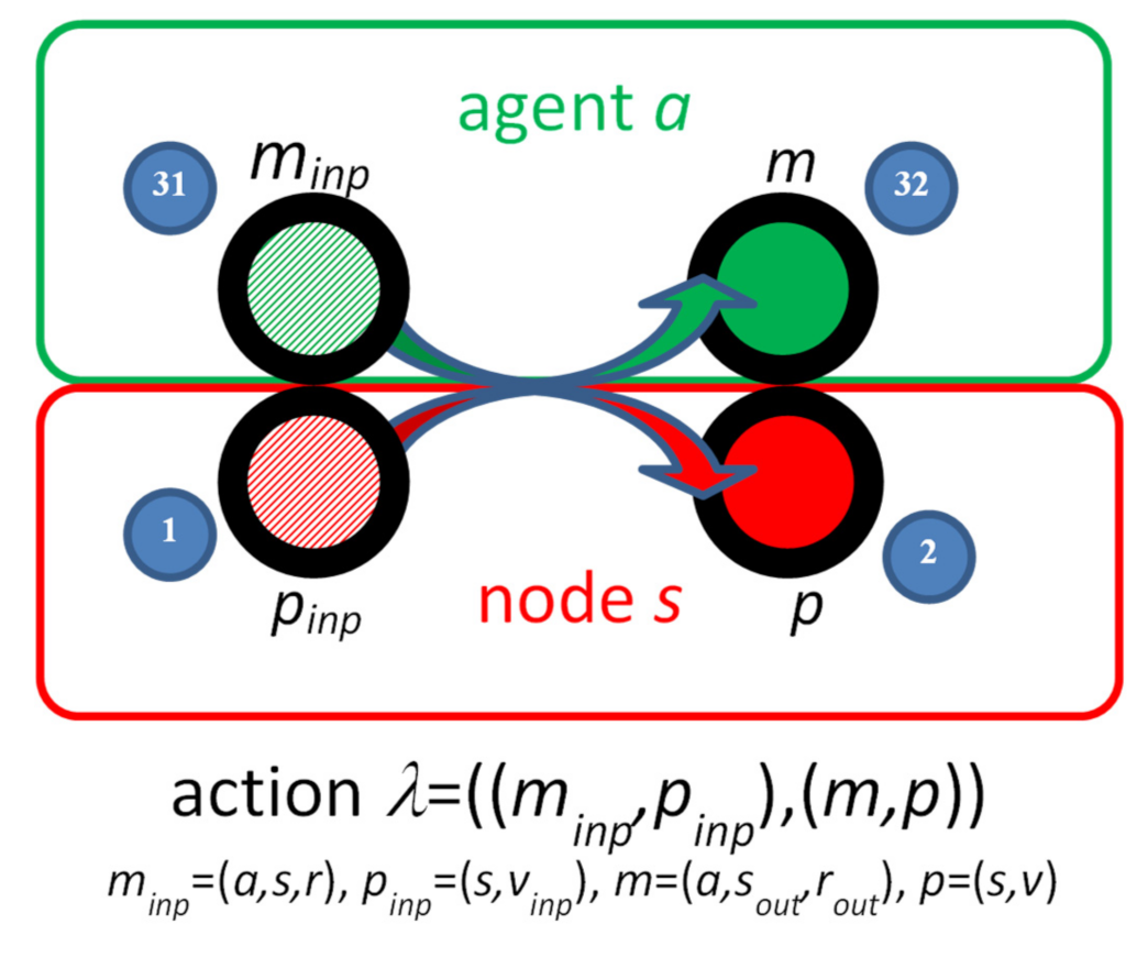
• Λ ⊂ (M × P) × (M × P)—set of actions

For the elements of Λ we use the prefix notation λ = ((m,p), (m′,p′)) ∈ Λ. The idea of the IMDS action is presented graphically in Figure 1. The elements of the action, in this and consecutive figures, are given as small blue circles with numbers. There are the references to those elements in the text, for example (1).

The agent’s message invokes an action on the node (the calculation step in a distributed environment) that can be performed in specific states of the node. Performing the action ‘consumes’ the message and state, and creates the next node state and the next agent message.

In the action λ = ((m,p), (m′,p′)) we say that:

• the pair (m,p) match (1,31);
• (m,p) is the input pair, (m′,p′) is the output pair (2,32);
• the state p is current, the message m is pending;
• p′ is the next state, m′ is the next message.

The definition must be supplemented by the initial sets of states and messages:

• P_ini ⊂ P – set of initial states
• M_ini ⊂ M – states of initial messages.

It should be noted that IMDS is not an automata-based model, although it can be represented as a collection of automata, in various ways; the paper [40] formally presents the conversion of IMDS to node automata or to agent automata. In the present article, we use some graphical notation informally, with node states as vertices and actions as transitions, because such notation is natural and makes it easier to express certain features of the IMDS. However, it should be remembered that such automata are only one of the possible interpretations; there are also others, such as the agent automata mentioned above, as well as pairs of synchronous automata (custodians and messengers [41]), or the non-automata interpretation as Petri nets shown in [21]. There is also an imperative language Rybu, compatible with IMDS, used by the student to verify their synchronization solutions [42]. Now, we are working on an even higher level language for web service composition. Please note that IMDS is only a set of actions over the quadruple Cartesian product (M × P) × (M × P). For programming purposes, these actions can be grouped on nodes, agents, or otherwise, which does not change the essence of the definition of formalism itself.

3.2. IMDS System Behavior

The behavior of the IMDS system is represented by labeled transition systems (LTS [38,39]), i.e., a rooted labeled directed graph.

LTS vertices are configurations that are sets of current states and pending messages. The root is the initial configuration, consisting of agents’ initial messages and nodes’ initial states. States and messages together are called items. LTS transitions are defined by actions, transforming their input configurations into output configurations.

• H = P ∪ M—set of items
• T_ini = P_ini ∪ M_ini—initial configuration
• T ⊆ H—configuration
• ∀_λ∈Λ λ = ((m,p),(m′,p′)) T_inp(λ) ⊃ {m,p}, T_out(λ) = T_inp(λ)\{m,p} ∪ {m′,p′}—obtaining T_out(λ) from T_inp(λ) for an action (31,1)→(32,2)
• LTS = ⟨N,N₀,W⟩, where
  • N is a set of vertices (configurations {T₀, T₁, …}, T_ini = T₀);
  • N₀ = T_ini is the root;
  • W is the set of directed labeled transitions, W ⊆ N × Λ × N, W = {(T_inp(λ),λ_i,T_out(λ) | λ_i∈ Λ, i = 1, …, ord(Λ)}.

The interleaving semantics of the system is assumed [43], i.e., exactly one action is executed at a time.

3.3. IMDS Processes

Processes are defined in the IMDS as action sequences. Intermediate elements link the actions in the sequence. If the intermediate elements are the states of a given node, then this is the process of that node, and the messages serve as a means of communication between processes. Conversely, if the messages of a given agent combine the actions of a process, then this is the process of this agent, and the states of the nodes are used to communicate processes. To do this, certain attributes must be assigned to the elements. Therefore, the elements are not atomic, as in the previous chapter. We redefine elements as tuples in four basic sets: nodes, agents, values, and services.

The formal definition of IMDS for the purpose of processes extraction is as follows:

• S = {s₁, s₂, …, s_Ns}—finite set of nodes
• A = {a₁, a₂, …, s_Na}—finite set of agents
• V = {v₁, v₂, …, v_Nv}—finite set of values
• R = {r₁, r₂, …, r_Nr}—finite set of services

The nodes’ states are defined as pairs (node, value): p = (s,v), s ∈ S, v ∈ V, and the messages as triples (agent, node, service): m = (a,s,r), a ∈ S, s ∈ S, r ∈ R. In such a formulation, a message is an invocation of a node’s service by an agent. An action is an execution of a service on a node in the context of an agent.

• P ⊂ S × V—set of states,
• M ⊂ A × S × R—set of messages,
• H = P ∪ M—set of items,
• Initial sets P_ini and M_ini, set of items H, configurations T and T_ini are defined over P and M, as before.

In order to terminate the agent, we add a new type of action, having a pair (message, state) on the input, but only a singleton (state) on the output. The definition of the action relation in terms of agents, nodes, values, and services is as follows:

• Λ ⊂ (M × P) × (M × P) ∪ (M × P) × (P) | (m,p)Λ(m′,p′) ∨ (m,p)Λ(p′), m = (a,s,r) ∈ M, p = (s₁,v₁) ∈ P, m′ = (a₂,s₂,r₂) ∈ M, p′ = (s₃,v₃) ∈ P, s₁ = s, s₃ = s, a₂ = a

Thus, Λ is not strictly a relation, because it contains both quadruples and triples.

We define functions of m and p, appointing their node and agent: for m = (a,s,r), Ms(m) = s, Ma (m) =a, for p = (s,v), Ps(p) = s.

The previous definitions of T, T_inp, T_out, and LTS hold. The initial configuration contains exactly one state for every node and exactly one message for every agent: initial states of every node and initial message for every agent. For T_ini, ∀m₁,m₂ ∈ T_ini, m₁ ≠ m₂: Ma(m₁) ≠ Ma(m₂); ∀p₁,p₂ ∈ T_ini, p₁ ≠ p₂: Ps(p₁) ≠ Ps(p₂).

The definitions of node and agent processes are as follow:

• B(s) = {λ ∈ Λ | λ = (((a,s,r),(s,v)), ((a,s′,r′),(s,v′))) ∨ λ = (((a,s,r),(s,v)), ((s,v′))), s′ ∈ S, a ∈ A, v,v′ ∈ V, r,r′ ∈ R}—node process of the node s ∈ S,
• C(a) = {λ ∈ Λ | λ = (((a,s,r),(s,v)), ((a,s′,r′),(s,v′))) ∨ λ = (((a,s,r),(s,v)), ((s,v′))), s,s′ ∈ S, v,v′ ∈ V, r,r′ ∈ R}—agent process of the agent a ∈ A,

The system views are

• B = {B(s₁),B(s₂),…,B(s_Ns) | s_i ∈ S}—the node view (decomposition of the system to node processes),
• C = {C(a₁),C(a₂),…,C(a_Na) | a_i ∈ A}—the agent view (decomposition of the system to agent processes).

3.4. Automated Deadlock and Termination Identification in IMDS

For model checking, atomic Boolean formulas must be assigned to any configuration in the LTS:

• D_s—true in all configurations, where at least one message is pending at the node s,
• E_s—true in all configurations, where at least one action is prepared at the node s.
• D_a—true in all configurations, where a message of the agent a is pending,
• E_a—true in all configurations, where the action is prepared with a message of the agent a,
• F_a—true in all configurations, where a terminating action (with a message of the agent a on input) is prepared.

Model checking formulas—CTL version [6]:

• communication deadlock in node s: EF AG(D_s ∧ ¬E_s)—a configuration is reachable in which a message is pending at the node s, but from this configuration on, no action will be prepared on node s;
• node s idle: AF AG(¬D_s)—there is a configuration after which no message will arrive at s;
• resource deadlock in the agent a: EF AG(D_a ∧ ¬E_a)—a configuration is reachable in which a message of the agent a is pending but from this configuration on, the message will not match any state;
• termination of agent a: AF(F_a)—a terminating action of agent a is inevitable.

It should be noted that the above deadlock detection formulas are defined for individual processes (nodes or agents). They allow the finding of partial deadlocks (also referred to as local deadlocks in the literature) concerning a limited number of processes, not just total deadlocks (also known as global deadlocks). The total node deadlock can be found in IMDS by means of the formula EF AG(∀s ∈ S: D_s ∧ ¬E_s), and the total agent deadlock by means of the equivalent formula over agents. Typical static deadlock detection methods only detect total deadlock [2]. There are methods for detecting partial deadlocks, but at the cost of limiting the allowed process shape or explicitly specifying a deadlock using model-specific formulas. Finding a partial deadlock using general formulas is an original achievement in IMDS.

The above IMDS definition supports all of the features of the distributed system:

• communication duality: Any system can be broken down into node processes that communicate via messages (the output state of the action is the carrier of the node process, while the output message is the means of communication) or agent processes communicating through the states of the nodes (the output message is the carrier agent process, while the output state is the means of communication);
• locality: Each action on a node is dependent on the node’s current state, and one of a set of pending messages on that node; no incident from outside (except messages received by the node) can affect the behavior of the node;
• autonomy: each node independently decides which of the defined actions can be performed in the current situation; in other words, the nodes decide for themselves if, and when, the messages are accepted and what actions they will cause;
• asynchrony: the node receives a message when it is ready for it; otherwise the message is pending; there are no synchronous operations in the model, such as simultaneous transitions on shared symbols in Büchi automata [3] or timed automata [18], and no joint operations of nodes or agents; synchronous sending and receiving operations in CSP [44], Occam [45], or Uppaal Timed Automata [14], synchronous operations on the complementary input and output ports in CCS [44]; node and agent autonomy is implemented using asynchronous operations: sending a message to a node or setting a new node state for subsequent agent operations are the only ways to influence the behavior of nodes and agents;
• asynchronous channels: communication between nodes is one-way (communication in the opposite direction has its separate channel) and may appear synchronous because the message appears on the receiving node immediately after it is sent; however, asynchrony is modeled by the possibility of deferring the message’s acceptance; the message can wait a long time, even forever, before being accepted;
• automated verification: the four above-mentioned temporal formulas are used to locate communication deadlocks in the processes of individual nodes, idleness of nodes, deadlocks over resources in agent processes, and agent termination, regardless of the structure of the verified system; therefore, they form the basis of the design of the automatic Dedan verifier, which can be used without knowledge of time logic and model checking.

We will present the translation of timed IMDS to timed automata for two reasons. First, TA is the most commonly used formalism on concurrent systems; thus, the translation of T-IMDS to TA gives a formal definition of its semantics. Second, the Dedan model checker is based on explicit state space representation, allowing for verification of small and medium systems. Large systems, in which more than ten nodes with complicated structures are contained, are exported from Dedan to Uppaal model checker for their verification.

4. Timed IMDS (T-IMDS)

In the timed version of IMDS, all of the mentioned functions are preserved: the duality of communication, locality, autonomy, asynchrony, and automated verification. In addition, time restrictions, which can last over time, are imposed on elements of the distributed system:

• time durations of actions (fixed or range),
• time delays of inter-node channels (fixed or range).

This collection of time constraints is smaller than the possibilities offered by TA; for example, time invariants of locations implementing staying in states, and differences of clock values are not included in T-IMDS. However, the selected time-related functions are best addressed to modeling distributed systems: differences in clock values (between distributed nodes) assume some knowledge about the global state. Limiting the time spent in locations implementing node states cannot be mixed with operations on urgent channels that are needed for the implementation of asynchronous channels (see later in this chapter); this is a limitation of the UTA syntax.

The behavior of a distributed system is determined by its LTS. All possible sequences of actions are included in the LTS. Time constraints are intended to exclude certain behaviors, due to violations of time restrictions imposed on actions and channels. Such a modification of the system behavior may, for example, prevent a deadlock (exclude the sequence leading to a deadlock) or cause a deadlock (for example, a process that is intended to meet a given condition may become stuck prematurely due to time constraints).

4.1. Syntax

The syntax of timeless IMDS is simply a set of actions of the form (((a,s,r),(s,v)),((a,s′,r′),(s,v′))), plus agent-terminating actions (((a,s,r),(s,v)),((s,v′))), denoted {a.s.r, s.v} -> {a.s′.r′, s.v′} and {a.s.r, s.v} -> {s.v′}. To simplify the description, in the description of timed formalism we will omit the agent terminating actions. An additional syntax is used to define types of nodes and agents, their parameterization, declaration of node and agent variables, and their initialization.

In notation, the dispersion of the duration of the action, in the form of a range with a lower and upper bound, is inserted between the input and output items of the action, for example a duration range (z1,z2) for an action λ has the form: λ = ((m_inp,p_inp),(m,p)) = (((a,s,r),(s,v)),(z1,z2)((a,s_out,r_out),(s,v_out))). A range can have open or closed bounds: (z1,z2), <z1,z2), (z1,z2>, <z1,z2>. The notation of ranges is taken from T-IMDS, where round parentheses denote open bounds and angle brackets denote closed bounds. The timed action has the form {a.s.r, s.v} -> (z1,z2){a.s’.r’, s.v’} in T-IMDS source format, and angle brackets can be applied for closed bounds.

Channel delays are defined as ranges in channels {...} phrase, for all channels: (d1,d2), for all channels leading to a given node s, or all elements of a vector s[…] of nodes: –>s(d1,d2), or between individual nodes: s1–>s2(d1,d2). In addition, individual elements of node vectors can be used: –>s[2](d1,d2), s1[1]–>s2[3](d1,d2).

An example of a system consisting of two distributed semaphores and two nodes using those semaphores, specified in T-IMDS in the input form of the Dedan verifier, is presented Listing 1 (the nodes are called servers in the IMDS language).

Listing 1.

 1.system two_semaphores;

 2. server: sem(agents a1,a2;servers sa1,sa2),

 3. services {wait, signal},

 4. states {up, down},

 5. actions {

 6. {a1.sem.wait, sem.up} → (2,3>{a1.sa1.ok_wait, sem.down}

 7. {a1.sem.signal, sem.down} → (2,3>{a1.sa1.ok_signal, sem.up}

 8. {a2.sem.wait, sem.up} → (2,3>{a2.sa2.ok_wait, sem.down}

 9. {a2.sem.signal, sem.down} → (2,3>{a2.sa2.ok_signal, sem.up}

10. };

11. server: proc(agents Ag;servers sem[2]),

12. services {start, ok_w, ok_s},

13. states {initial, first, second, end},

14. actions {

15. {Ag.proc.start, proc.initial} -> <0>{Ag.sem[1].wait, proc.first},

16. {Ag.proc.ok_w, proc.first} -> <0>{Ag.sem[2].wait, proc.second},

17. {Ag.proc.ok_w, proc.second} -> <0>{Ag.sem[1].signal, proc.first},

18. {Ag.proc.ok_s, proc.first} -> <0>{Ag.sem[2].signal, proc.second},

19. {Ag.proc.ok_s, proc.second} -> <0>{proc.end},

20. };

21. servers semaphore[2]:sem,process[2]:proc;

22. agents Ag[2]; 

23. channels {<0>};

24. init -> {

25.  process[1](Ag[1],semaphore[1,2]).initial,

26.  process[2](Ag[2],semaphore[2,1]).initial,

27. <j=1..2> semaphore[j](Ag[1..2],process[1..2]).up,

28. <j=1..2> Ag[j].process[j].start,

29. }.

This is the specification in the node view. It is simply a collection of actions on particular nodes. A set of node type specifications defines a system (enclosed by server …};—lines 2–10, 11–20), node and agent instance (variable) declarations (agents …, servers …—lines 21,22), and an initial configuration phrase (init → lines 24–29). A node type heading contains a set of formal parameters, such as the agents and nodes employed in the node type’s activities. Formal parameters, such as Ag[2] and sem[2], can be vectors (line 11). A set of services (lines 3,12), a set of states (lines 4,13), and a set of actions are allocated to each node (lines 6–9, 15–19). An action λ = (((a,s,r),(s,v)), ((a,s_out,r_out),(s,v_out))) has the form {a.s.r, s.v} → (x,y){a.sout.rout, s.vout}. The time bounds (x,y) limit the action duration. Services and states can be vectors (not in this example, see the source code of AVGS system in Section 7.2). Repeaters may precede actions in a node type definition for its compactness (for example, in an AVGS system Section 7.2, 2 repeaters are used for some actions). Vectors can be used to arrange node and agent instances (lines 21,22). The channels phrase (line 23) specifies channel delays, in this example, the channels have no delay. The delays can be assigned to each channel individually. Actual parameters are bound to formal parameters in the initialization part (line 24). The nodes’ initial states and the agents’ initial messages are also assigned.

4.2. Semantics

The execution of the action is divided into three phases for states and four phases for messages, as shown in Figure 2. The complete environment of the action λ, with the actions delivering the input items m_inp and p_inp, is presented in Figure 3. Of course, more than one action can deliver an input item of the action. Due to non-determinism, the action can deliver its output items, m and p, to multiple consecutive actions. The phases of the action are as follows:

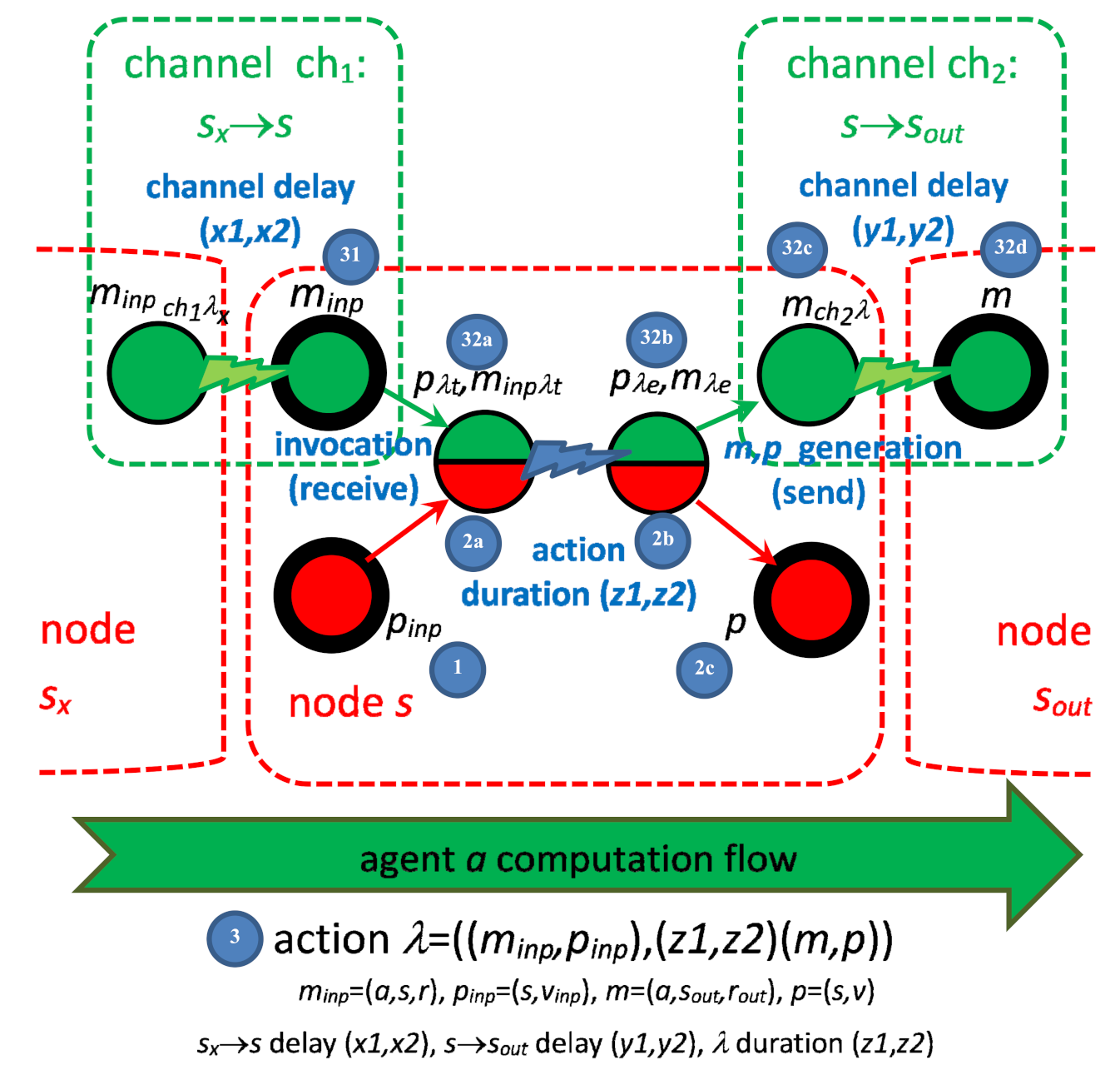
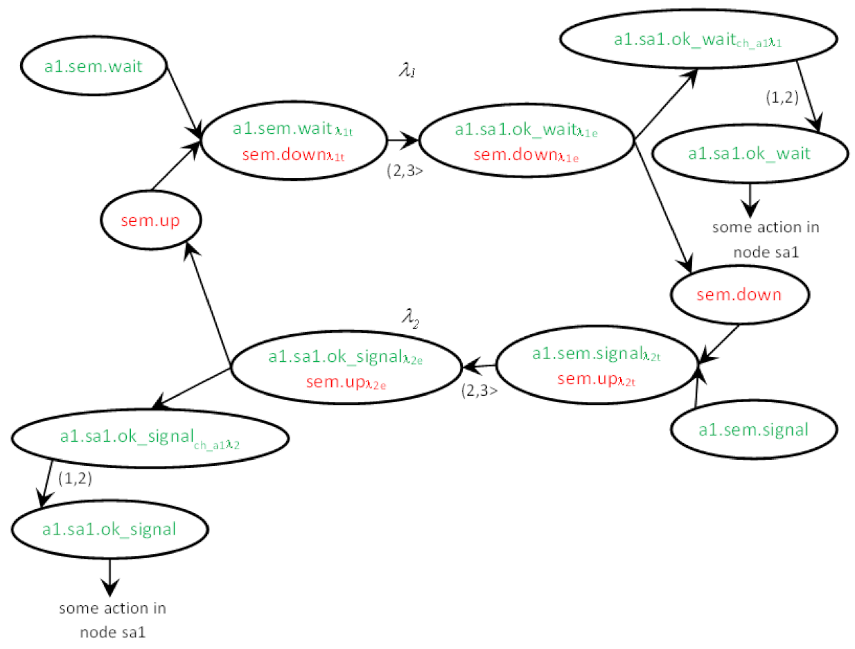
• The current input state p_inp (1) and pending input message m_inp (31) match; therefore, they can invoke the action λ = ((m_inp,p_inp),(m,p)): (31,1)→(32d,2c). If multiple actions are enabled in a node, the choice is nondeterministic. The first phase (31,1)→(32a,2a) is a reception of the message m_inp and invocation of the action.
• Time duration of the action begins, which lasts between t_{λ min}(λ) and t_{λ max}(λ). Counting the time duration is the second phase (32a,2a)→(32b,2b).
• When the time duration ends, the new pair of (m,p) is generated (32b,2b)→(32c,2c). From this moment, the state p is available for invoking the next action in the node. The message m is sent to the target node, and it must be propagated to become accessible.
• The last phase is message delivery, in which the channel delay between t_{ch min}(ch) and t_{ch max}(ch) is counted (32c)→(32d). After the delay, the message m becomes available for invocation of the next agent action, in the target node with its current state.

The semantics of T-IMDS (timed LTS) is:

• For every action λ = ((m_inp,p_inp),(m,p)) (3), the range bounds of action duration t_{λ min}(λ) and t_{λ max}(λ) are defined.
• The set of channels CH of the form ch = (a,s_inp→s) are defined: ∀λ = ((m_inp,p_inp),(m,p)): ∃ ch: ch = (Ma(m_inp), Ms(m_inp)→Ms(m)). Totally K channels, indexed 1, …, K. The channel transmitting the output message of the action λ is denoted ch_λ.
• For every ch, the range bounds of channel delay t_{ch min}(ch), t_{ch max}(ch) are defined.
• Delay time is defined for a channel between given nodes; therefore, for all agents sending messages along the channel, the range of delay is equal: ∀a₁,a₂: ∀ch₁ = (a₁, s_inp→s), ch₂ = (a₂, s_inp→s): t_{ch min}(ch₁) = t_{ch min}(ch₂) ∧ t_{ch max}(ch₁) = t_{ch max}(ch₂); however, this does not influence the shape of the LTS.
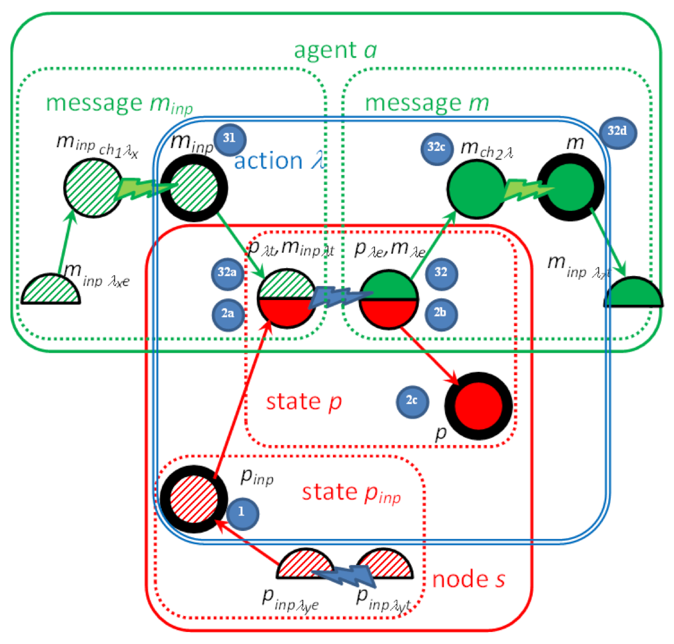
• A timed configuration consists of messages, states, their derivatives, node time values ct_s, and channel time values ct_ch: T_t = (T = {m_tai, p_tsj | i = 1, …, Na, j = 1, …, Ns, m_tai ∈ M_t, p_tsi ∈ P_t}, ct_s1, …, ct_sNs, ct_ch1, …, ct_chK), where Na is the number of agents and Ns is the number of nodes. T is called a set of items.
• The set of states p (1,2b) and derivatives p_λt (2a), p_λ (2b)_e: P_t = {p_i, p_iλjt, p_iλje | I = 1, …, card(P), j = 1, …, card(λ), λ_j = ((m_inp,p_inp),(m,p_i)) ∈ Λ, p_iλjt = (p_i,λ_j), p_iλje = (p_i,λ_j)}
• The set of messages m (31,32d) and derivatives m_λt (32a), m_λe (32b), m_chλ (32c): M_t = {m_i, m_iλjt, m_iλje, m_ichλj | i = 1, …, card(M), j = 1, …, card(Λ), k = 1, …, K, λ_j = ((m_inp,p_inp),(m_i,p)) ∈ Λ, m_iλjt = (m_i,λ_j), m_iλje = (m_i,λ_j), m_ichλj= (m_i,ch_λj,λ_j) }.
• For λ = ((m_inp,p_inp),(m,p)) we define that Ps(p_λt) = Ps(p_λe) = Ps(p), Ms(m_λt) = Ms(m_λe) = Ms(m_chλ) = Ms(m), Ma(m_λt) = Ma(m_λe) = Ma(m_chλ) = Ma(m).
• Each p_λt has two attributes: t_{λ min}(p_λt) and t_{λ max}(p_λt).
• Each m_chλ has two attributes: t_{ch min}(m_chλ) = t_{ch min}(ch_λ) and t_{ch max}(m_chλ) = t_{ch max}(ch_λ).
• The root vertex in the LTS is the initial timed configuration is T_0t = (T₀ = {m_0a1, …, m_0aNa, p_0s1, …, p_0sNs | m_0ai∈M₀, p_0si ∈ P₀}, 0, …, 0, 0, …, 0).

The vertices in the LTS can contain three types of pair and a singleton causing the progress transitions (0-time transitions):

12.

(m_inp,p_inp) (31,1) is the input pair of an action λ,

13.

(m_inpλt,p_λt) (32a,2a) for a transition ending the time duration of the action λ,

14.

(m_λe,p_λe) (32b,2b) for generation of the output pair (m,p) of the action λ,

15.

(m_chλ) (32c) for a transition ending the time delay of the message m generated in the action λ.

In addition, we have a pair and a singleton causing the timed transitions:

16.

(m_inpλt,p_λt) (32a,2a) for a timed transition modeling sub-periods of time in the action duration of the action λ,

17.

(m_chλ) (32c) for a timed transition modeling sub-periods of time in the time delay of the message m generated in the action λ;

In execution of the action λ, the following pairs occur in some configurations in the LTS: (m_inp,p_inp), (m_inpλt,p_λt), (m_λe,p_λe), (m_chλ,p). Finally, m is not related to p or any derivative of p, because it takes some time for m to become operational, after channel delay. However, it can occur in a pair with p if the node does not begin execution of any action during the message m passing through the channel.

The transitions in the LTS are

18.

reception/invocation transition (31,2)→(32a,2a)—for T_t: (∃{m_inp,p_inp} ⊂ T: ∃λ ∈ Λ: λ = ((m_inp,p_inp),(m,p))) ⇒ T’_t = (T\{m_inp,p_inp} ∪ {m_inpλt,p_λt}, previous ct_s1,…,ct_sNs except c_{Ps(p inp)} := 0, previous ct_ch1,…,ct_chK);

19.

generation/send transition (of a new m and p) (32b,2b)→(32c,2c)—for T_t: (∃{m_λe,p_λe} ⊂ T: λ = ((m_inp,p_inp),(m,p))) ⇒ T’_t = (T\{m_λe,p_λe} ∪ {m_chλ,p}, previous ct_s1, …, ct_sNs, previous ct_ch1, …, ct_chK except c_chλ := 0);

20.

two transitions—action duration timed transition (32b,2b)→(32b,2b) and duration end timeless transition (32b,2b)→(32c,2c)—for T_t: ¬(∃ {m_inp,p_inp} ⊂ T: ∃λ ∈ Λ: λ = ((m_inp,p_inp),(m,p))) ∧ //no action to invoke ¬(∃ {m_λe,p_λe} ⊂ T: λ = ((m_inp,p_inp),(m,p))) ∧ // no message to generate (∃ {m_inpλt,p_λt} ⊂ T) | s=Ps(p_λt) ⇒ (t_{λ min}(λ) < ct_s < t_{λ max}(λ) ⇒ T’_t = (T\{m_inpλt,p_λt} ∪ {m_λe,p_λe}, previous ct_s1,…,ct_sNs except c_s := 0, previous ct_ch1,…,ct_chK), //action duration ended (ct_s<t_{λ max}(λ) ⇒ T″_t = (T, c_si := previous ct_si + δ, i = 1..Ns, c_chj := previous ct_chj + δ, j = 1..K));

21.

two transitions—channel delay timed transition (32c)→(32c) and delay end timeless transition (32c)→(32d)—for T_t: ¬(∃ {m_inp,p_inp} ⊂ T: ∃λ ∈ Λ: λ = ((m_inp,p_inp),(m,p))) ∧ //no action to start ¬(∃ {m_λe,p_λe} ⊂ T: λ = ((m_inp,p_inp),(m,p))) ∧ // no message to generate (∃ m_chλ∈T ) ⇒ (t_{ch min}(ch_λ) < ct_ch < t_{ch max}(ch_λ) ⇒ T’_t = (T\{m_chλ} ∪ {m}, previous ct_s1, …, ct_sNs, previous ct_ch1,…,ct_chK except c_chλ := 0)), //channel delay ended (ct_ch < t_{ch max}(m_chλ) ⇒ T″_t = (T, c_si:= previous ct_si + δ, i = 1..Ns, c_chj := previous ct_chj + δ, j = 1..K)).

22.

If multiple transitions come out of an LTS vertex, the choice is nondeterministic. However, if both reception/generation transition and duration/delay end transition are possible in the current configuration, the latter is not included into LTS.

23.

The general limit for δ in the parallel timed transitions is that for all ct_si in T_t, λ₁ = ((m_1inp,p_1inp),(m₁,p₁)), Ps(p_1inp) = s_i, p_λ1t ∈ T, and all ct_chλ2 in T_t, λ₂ = ((m_2inp,p_2inp),(m₂,p₂)), m_chλ2 ∈T, δ < min(t_{λ max}(p_λ1t)–ct_si, t_{ch max}(ch_λ2)–ct_chλ2). In every inequality t_min < ct, ct < t_max, the relation should be replaced by ≤ if the corresponding range bound is closed. If all t_{λ max}(p_λ1t) and all t_{ch max}(m_chλ2) in T_t are for closed upper bounds of time ranges, then the relation in the inequality < for δ should be replaced by ≤.

The latter condition says that we must not exceed the upper bound of any remaining action duration/channel delay.

5. Uppaal Timed Automata

5.1. The Syntax of Uppaal TA

A collection of timed automata and real-valued clocks are commonly used to define parallel systems. We expand the concept to include variables that can enable transitions and be allocated to transitions to conform with Uppaal TA.

An Uppaal timed automaton UTA is a tuple (L, l₀, Z, CH, Q, E, J_l, O, Ō₀) where

• L= {l₀, l₁, …} is a finite set of locations,
• l₀ ∈ L is an initial location,
• Z = {c₀, c₁, …} is the set of clocks,
• CH is a set of symbols called channels,
• Q denotes a set of labels (interpreted as actions on transitions, do not confuse with IMDS actions), they represent send and receive operations on a channel: ch!, ch?, ch ∈ CH; outside the automaton, internal labels are ignored and replaced by τ,
• every location l ∈ L is mapped by J_l(l) to a set of valuations of clocks in Z, over a Cartesian product of ${ℝ}_{\ge 0}^Z$, for example, J_l(l) = {c₁-c₂ > 2}; Restriction. As in verification tools, e.g., Uppaal [14], we limit location invariants to downwards closed constraints of the form: x ≤ n or x < n where n is a natural number,
• O = {o₁, o₂, …} finite set of variables, for which we define:
  V_i = {v_i1, v_i2, …}—finite, integral set of values of variable oi ∈ O,
  P_V = V₁ × V₂ × … × V_ord(O)—a Cartesian product of values of variables o₁, o₂, …, o_ord(O) ∈ O,
  Ō = (v₁, v₂, …, v_ord(O)); v_i ∈ V_i; Ō ∈ P_V—vector of values of variables in O,
• Ō₀ = (v₁⁰, v₂⁰, …, v_ord(O)⁰)—initial vector of values of variables in O,
• E ⊆ L × Q × J_ll × 2^Z × 2^PV× F × L—set of transitions: e = (l, q, J_ll(l,l′), r, b, f, l′) ∈ E
  • J_ll is a set of functions for pairs l,l’∈L, every transition (l,l’) is mapped by J_ll(l,l′) to a set of valuations of clocks in Z over a Cartesian product of ${ℝ}_{\ge 0}^Z$, just as J_l(l) for a location l,
  • r ∈ 2^Z indicates a subset of clocks in Z that are reset on transition,
  • b ∈ 2^PV—set of vectors of variable values enabling a transition; Comment: typically b is presented as equalities and inequalities between variables in O and constants, connected by Boolean operators, for example (o₁ < 3) ∧ (o₂ ≥ 6),
  • F is a set of functions on variables in O, f ∈ F, f: P_V → P_V—unction assigning new values to the variables in O; f/i restricts this function to the value of variable o_i. Comment: In Uppaal TA, the function is given as a set of assignments o_i = expression over variables in O and integer constants (all other variables are left unchanged).

5.2. The Semantics of UTA

The Semantics of a UTA is:

Let (L, l₀, Z, CH, Q, E, J_l, O, Ō₀) be an UTA.

The semantics is defined as an LTS—Labeled Transition System ⟨Vertices, vertex₀, ▶⟩, where:

• Vertices ⊆ L × P_V × ${ℝ}_{\ge 0}^Z$ is the set of LTS vertices for the automaton UTA (because the term state is reserved for IMDS node states, we use the term vertex instead),
• vertex₀ = (l₀, Ō₀, u₀) ∈ Vertices is the initial vertex, u₀ maps all clocks c ∈ Z to 0.
• ▶ = ▶_t ∪ ▶_p is the transition relation such that:
  • (l, Ō, u) ▶_t (l, Ō, u+d) if ∀d’: 0 ≤ d′ ≤ d ⇒ u + d′ ∈ J_l(l)—timed transition,
  • (l, Ō, u) ▶_p (l′, Ō′, u′) if there exists e = (l, q, J_ll(l,l′), r, b, f, l′) ∈ E such that u ∈ J_ll(l,l′); u′ = [r ↳ 0]u and Ō ∈ b and Ō′ = F(Ō)—progress transition;

where

for d’ ∈ ${ℝ}_{\ge 0}^Z$, u + d′ maps each clock c in Z to the value u(c) + d′,

[r ↳ 0]u, r ⊂ Z, denotes the clock valuation, which maps each clock in r to 0 and agrees with u over Z\r.

5.3. Network of UTA

NUTA is a network of Uppaal timed automata over a common set of clocks and labels (actions), a common set of variables, and a common initial vector of their values. NUTA is itself a UTA, it is constructed in the following way:

NUTA = (L, l⁰, Z, CH, Q, E, J_l, O, Ō⁰) consists of n UTA, UTA_i = (L_i, l_i⁰, Z_i, CH_i, Q_i, E_i, J_li, O_i, Ō_i⁰) with i = 1, …, n. The individual elements of NUTA are:

• A set of locations is a Cartesian product L = L₁ × … × L_n, l ∈ L is a location vector l = (l₁, …, l_n), l_i ∈ L_i.
• l⁰ ∈ L is an initial location vector l⁰ = (l₁⁰, …, l_n⁰), l_i⁰ ∈ L_i.
• Z is a common set of clocks—a union of sets of clocks Z = Z₁ ∪ … ∪ Z_n.
• CH is a common set of channels—a union of sets of channels CH = CH₁ ∪ … ∪ CH_n, it can be ignored because the labels in Q disappear in the construction of NUTA.
• Q is a common set of labels—symbols on transitions: the labels on channels (ch!, ch?) disappear on the construction on NUTA (they are replaced by τ) according to the semantic rules given below.
• Location invariant functions are composed into a common function over location vectors J_l(l) = J_l1(l₁) ∧ … ∧ J_ln(l_n).
• O is a common set of variables (union of sets of variables O₁ ∪ … ∪ O_n), Ō—vector of their values, P_V—the Cartesian product of sets of values of all variables in O, Ō₀—a common vector of their initial values.

The NUTA graph is constructed in such a way that transitions between the compound locations of NUTA (starting from initial compound location l⁰) are chosen as common timed transitions, interleaved progress transitions having labels, and common progress transitions of pairs of UTA with matching ch! and ch? labels, interleaved with the transitions of all other UTA. Additionally, the set of transitions in NUTA can be restricted by conjunctions of time invariants J_l in timed transitions, and by conjunctions of functions J_lli and intersections of b_i. Last, all those rules met by the semantics of NUTA are expressed as the LTS of a set UTA below.

5.4. The Semantics of the Network of UTA

Let UTA_i = (L, l⁰, Z, CH, Q, E, J_l, O, Ō⁰).

Let l⁰ = (l₁⁰, …, l_n⁰) be the initial location vector.

l[l_i/l_i′] denotes the location vector where l_i′ replaces the i^th element l_i of L.

The semantics of a network on n UTA is defined as an LTS ⟨Vertices, vertex₀, ▶⟩, where:

• Vertices = (L₁ × …× L_n) × P_V × ${ℝ}_{\ge 0}^Z$ is the set of global LTS vertices,
• vertex₀ = (l₀; Ō₀; u₀) ∈ Vertices is the initial vertex, u₀ maps all clocks c ∈ Z to 0,
• ▶ = ▶_t ∪ ▶_p ∪ ▶_!? is the transition relation defined by:

  3a.

  (l, Ō, u) ▶_t (l, Ō, u + d) if ∀_d′ 0 ≤ d’ ≤ d ⇒ u + d′ ∈ J_l(l)—timed transition,

  3b.

  (l, Ō, u) ▶_p (l[l_i/l_i′], Ō′, u′); if there exists (l_i, τ; J_lli(l_i,l_i′), r_i, b_i, f_i, l_i′) ∈ E_i such that u ∈ J_lli(l[l_i/l_i′]); u′ = [r_i ↳ 0]u and Ō ∈ b_i and Ō′ = f_i(Ō)—progress transition,

  3c.

  (l, Ō, u) ▶_!? (l[l_j/l_j′, l_i/l_i′], Ō′, u′) if there exist two transitions (l_i, ch?, J_lli(l_i,l_i′), r_i, b_i, f_i, l_i′) ∈ E_i and (l_j, ch!, J_llj(l_j,l_j′), r_j, b_j, f_j, l_j′) ∈ E_j such that u ∈ J_ll(l[l_j/l_j′, l_i/l_i′]), u′ = [r_i ∪ r_j ↳ 0]u and Ō ∈ b_i and Ō ∈ b_j—synchronization transition (a special kind of progress transition), new values of variables in O are calculated:

  • for every o_k ∈ O, f_i(o_k) = v_k and f_j(ok) = v_k′ or f_j(o_k) = v_k and f_i(o_k) = v_k′ Comment: At least one of the functions f_i, f_j must be an identity function for a given variable that returns the same value as its argument (it is disregarded); the other must be in effect (it gives the variable’s new value). This criterion prohibits incoherent assignments to the same variable in the automata UTA_j and UTA_k; it is met by the construction in the translation of T-IMDS to UTA, as an assignment is applied in only one of the pair’s automata;

• If both ▶_t and ▶_!? are possible from given vertex (l; Ō; u), then ▶_t is not inserted into LTS,
• If both ▶_p and ▶_!? are possible from given vertex (l; Ō; u), then ▶_p is not inserted into LTS; Comment: In this way, Uppaal urgent channels are achieved; only such channels are applied in the translation of T-IMDS to UTA,
• If two transitions are possible, the choice is non-deterministic (however, both are inserted into LTS because it defines all possible behaviors).

6. Translation of T-IMDS to Timed Automata

6.1. Example

To explain the translation rules, let us concentrate on the actions of the sem node from the example in Section 5.1, with actions duration (2,3>). It implements wait and signal services. Two agents, a1 and a2, use the semaphore. Each agent comes from its private node: sa1 for a1, and sa2 for a2. The time constraints are given in Listing 2.

Listing 2.

 5. actions {

 6. {a1.sem.wait, sem.up} → (2,3>{a1.sa1.ok_wait, sem.down}   //λ₁

 7. {a1.sem.signal, sem.down} → (2,3>{a1.sa1.ok_signal, sem.up} //λ₂

 8. {a2.sem.wait, sem.up} → (2,3>{a2.sa2.ok_wait, sem.down}   //λ₃

 9. {a2.sem.signal, sem.down} → (2,3>{a2.sa2.ok_signal, sem.up} //λ₄

10. }

For every node s, an Uppaal timed automaton s is declared. In fact, an UTA type is defined just as a node type can be defined in T-IMDS, but this is a syntactic manipulation for the programmer’s convenience. The UTA variable is equipped with its own clock c_s and a set of locations and derivatives, in the example c_sem, up, up_λ2t, up_λ2e, up_λ4t, up_λ4e, down, down_λ1t, down_λ1e, down_λ3t, down_λ3e. For storing the service name invoked by messages, variables a1_sem and a2_sem are applied for the agents in sem. For nodes sa1 and sa2, variables a1_sa1 and a2_sa2 are applied. The set of values for a1_sem and a2_sem variables is {none, sem_wait, sem_signal}, for a1_sa1 {none, sa1_ok_wait, sa1_ok_signal}, and a2_sa2 {none, sa2_ok_wait, sa2_ok_signal}. The node clocks are c_sem, c_sa1, and c_sa2.

The initial state is chosen outside the node type, in the init section, to allow different instances to have different initial states; up or down in our example. Assume that the node sem has the initial state up. The set of UTA locations and transitions for automaton sem is as follows (for comparison in Boolean expressions over variables we use a double equals operator, which follows the Uppaal rule; for assignment and clock reset, we use equals character preceded by a colon (:=) to clearly distinguish it from comparison and to agree with Uppaal):

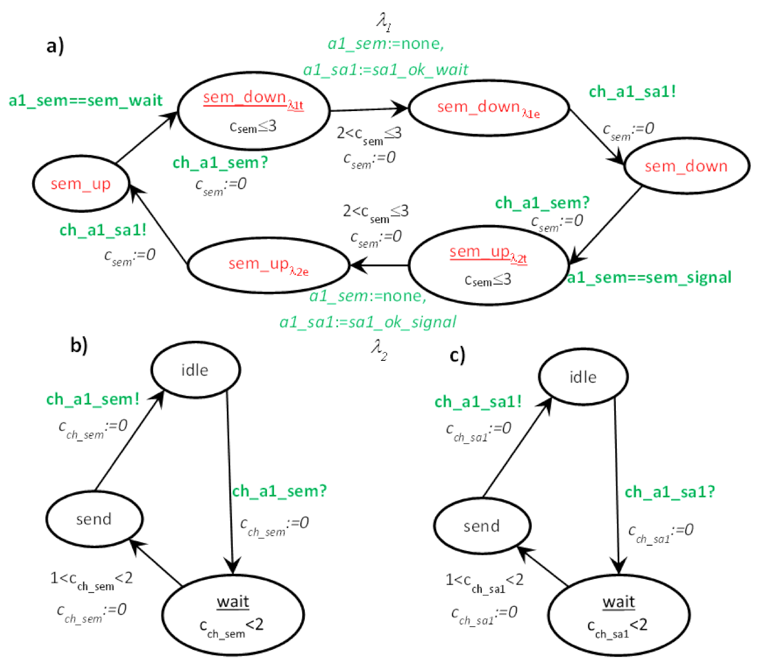
• (31,1) location down: initial location—no, time invariant—no (4),

  -

  (31,1)→(32a,2a) transition: next location—up_λ2t, condition—a1_sem==sem_signal, assignments—no, time constraint—no, clock reset—c_sem:=0, channel synchronization: ch_a1_sem? (4)→(8)→(5)

  -

  (31,1)→(32a,2a) transition: next location—up_λ4t, condition—a2_sem==sem_signal, assignments—no, time constraint—no, clock reset—c_sem:=0, channel synchronization: ch_a2_sem? (4)→(8)→(5)

• (32a,2a) location up_λ2t: initial location—no, time invariant—c_sem ≤ 3 (5),

  -

  (32a,2a)→(32b,2b) transition: next location—up_λ2e, condition—no, assignments—a1_sem:=none, a1_sa1:=sa1_ok_up, time constraint—2 < c_sem ≤ 3, clock reset—c_sem:=0, channel synchronization—no (5)→(9)→(6)

• (32b,2b) location up_λ2e: initial location—no, time invariant—no (6),

  -

  (32b,2b)→(32c,2c) transition: next location—up; condition—no, assignments—no, time constraint—no, clock reset—c_sem:=0, channel synchronization: ch_a1_sem_sa1! (6)→(10)→(7)

• (32a,2a) location up_λ4t: initial location—no, time invariant—c_sem ≤ 3 (5),

  -

  (32a,2a)→(32b,2b) transition: next location—up_λ4e, condition—no, assignments—a2_sem:=none, a2_sa2:=sa2_ok_up, time constraint—2 < c_sem ≤ 3, clock reset—c_sem:=0, channel synchronization—no (5)→(9)→(6)

• (32b,2b) location up_λ4e: initial location—no, time invariant—no,

  -

  (32b,2b)→(32c,2c) transition: next location—up; condition—no, assignments—no, time constraint—no, clock reset—c_sem:=0, channel synchronization: ch_a2_sem_sa2! (6)→(10)→(7)

• (2c) location up: initial location—no, time invariant—no (7),
• …etc.

6.2. Translation Rules

Since the channels leading from different nodes to the node s are combined together, we use the notation (a,→s) for the channel passing messages of the agent a to the node s. The rules for translation of λ = ((m_inp,p_inp),(m,p)), m_inp = (a,s,r), m = (a,s_out,r_out) are depicted in Figure 4, and message m transfer along the channel ch = (a,→s_out) from T-IMDS to UTA in Figure 5. Three channel versions are shown: (a) the basic form, (b) the 0-time channel without delay, and (c) the channel receiving messages of the agent coming from various nodes with different delays. Please do not mistake the wait location of a channel with the wait service offered by semaphores in the example. We numbered all the elements of T-IMDS and its UTA implementation to be referred to in the following translation rules:

• sever s ⇒ timed node automaton s with clock c_s (reset on every transition, used to count actions duration),
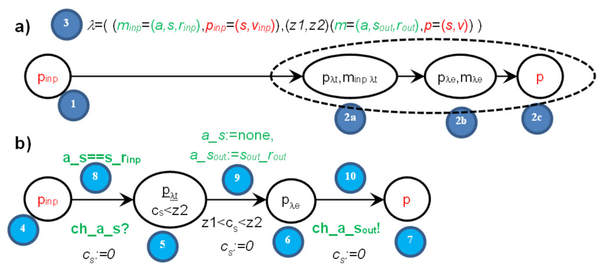
• state p of automaton s (1,2c) and derivatives (p_λt, p_λe) (2a,2b) ⇒ locations p, p_λt, p_λe in timed node automaton s (4,5,6,7),
• message m (32,32d) and derivatives (m_λt, m_λe, m_chλ) (32a,32b,32c) ⇒ pairs of message variable a_s values and locations of automaton s and automaton ch, details below,
• agent a → set of variables (for every node visited by the agent) {a_s₁, a_s₂, …} (8),
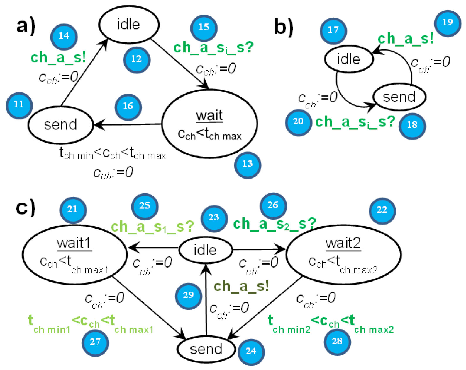
• channel ch ⇒ automaton ch (Figure 3) with clock c_ch (reset on every transition, used to count channel delay),
• message m_inp pending at the node s (1) ⇒ a_s == s_r (8), all other a_s_x == none, s_x ≠ s, channel ch in location send (11,18,24), variable a_s has a set of values {none, s_r, s_r₁, s_r₂, …} (8) (services r, r₁, r₂ distinguish between messages sent to the node s by the agent a),
• derivative item p_λt for action λ (duration running) (2a) ⇒ location p_λt (5),
• derivative item p_λe for action λ (duration ended) (2b) ⇒ location p_λe (6),
• message m_inp (stable message m_inp) (32) ⇒ pair (send,a_s==s_r); (8) location send in channel (a,→s) (11,18,24),
• derivative item m_inpλt for action λ ⇒ pair (p_λt, a_s == s_r) (5,8,14/19/29); note that a_s_out==none,
• derivative item m_λe for action λ ⇒ pair (p_λe, a_s_out == s_out_r_out) (6,9); note that a_s == none,
• derivative item m_chλ for action λ ⇒ location wait of the channel ch automaton (15/20/25/26); note than a_s == none, a_s_out == s_out_r_out (9),
• configuration T ⇒ set of locations of node automata representing node states and derivatives and values of pairs (location of a node automaton s_x/channel automaton ch_z, value of a_y_s_x) representing messages and derivatives,
• actual value of action duration in node s/channel ch delay in T_t—the value of the clock c_s/clock c_ch (9/27/28),
• duration range lower bound t_{λ min}(λ) ⇒ lower bound of time constraint of the transition p_λt→p_λe: t_{λ min}(λ) < c_s (9),
• duration range upper bound t_{λ max}(λ) ⇒ upper bound of time constraint of the transition p_λt→p_λe: c_s < t_{λ max}(λ) (9) and of time invariant of location p_λt: c_s < t_{λ max}(λ) (5),
• delay range lower bound t_{ch min}(ch) ⇒ lower bound of time constraint of the transition wait→send of the channel automaton, t_{ch min}(ch) < c_ch (16/27/28),
• delay range upper bound t_{ch max}(ch) ⇒ upper bound of time constraint of the transition wait→send of the channel automaton, c_ch < t_{ch max}(ch) (16/27/28) and of time invariant of wait location: c_ch < t_{λ max}(ch) (13/21/22),
• action λ (3), (31,1)→(32a,2a)→(32b,2c)→(32c,2c), (32c)→(32d) ⇒ sequence: message and state(m_inp,p_inp)-receive transition(m_inp,p_inp)→(m_inpλt,p_λt)-duration location(p_λt)-timed transitions(action duration in p_λt)-end of duration transition(m_inpλt,p_λt)→(m_λe,p_λe)-end of duration location(p_λe)-send transition(m_λe,p_λe)→(m_chλ,p), (11/18/24,4) → (14/19/29,8) → (12/17/23,5) → (9) → (12/17/23,6) → (15/20/25/26,10) → (13/18/21/22,7),
• receive transition (m_inp,p_inp)→(m_inpλt,p_λt) (31,1)→(32a,2a) ⇒ channel automaton ch_as = (a,→s) in location send, node s automaton in location p_inp, urgent channel synchronization (ch_a_s! on (m_inp,p_inp)→(m_inpλt,p_λt), ch_a_s? on send→idle), condition a_s == s_r fulfilled, on transition c_s is reset to 0, (11/18/24,4) → (14/19/29,8) → (12/17/23,5),
• end of action duration transition (m_inpλt,p_λt)→(m_λe,p_λe) (32a,2a)→(32b,2b) ⇒ node s automaton in location p_λt, clock c_s value t_{λ min}(λ) < c_s < t_{λ max}(λ), on transition a_s := none, a_s_out == s_out_r_out, c_s is reset to 0, (12/17/23,5) → (9) → (12/17/23,6),
• generation of next m,p and send transition (m_λe,p_λe)→(p,m_chλ) (32b,2b)→(32c,2c) ⇒ node s automaton in location p_λe, channel ch automaton in location idle, urgent channel synchronization (ch_a_s_s_out! on (m_λe,p_λe)→(p,m_chλ), ch_a_s_s_out? on idle→wait), (12/17/23,6) → (15/20/25/26,10) → (13/18/21/22,7),
• advancing duration of an action (32b,2b)→(32b,2b) or channel delay (32c)→(32d) ⇒ timed transitions—within time invariants of all locations with time invariant—to a next time region, limited by outgoing transitions time range upper bounds, t_{λ max} for action durations in p_λt locations (5–9), and t_{ch max} for channel delays in wait locations (13–16/21–27/22–28),
• asynchronous channel between nodes ch (32c)→(32d) ⇒ an asynchronous channel is compound of two synchronous urgent channels (Figure 5); asynchronous channel is inactive in the idle location (12/17/23); the signal that the message is ready is obtained from the sending automaton via input urgent channel ch_a_s_out: urgent channel synchronization (ch_a_s_out!, ch_a_s_out?) (15/20/25/26); then, the time delay is counted in the wait location (13/21/22); it lasts between t_{ch min} and t_{ch max}, as the transition ending the channel delay is followed for clock values c_ch t_{ch min}(ch) < c_ch < t_{ch max}(ch) (16/27/28); finally, the signal sending the message to the target automaton via output urgent channel ch_a_s_s_out is issued: urgent channel synchronization (ch_a_s_s_out!, ch_a_s_s_out?) (14/19/27/28); if the receiving s automaton is not ready to accept the message—the synchronization on ch_a_s is deferred: a message is pending (11/18/24); an own local clock c_ch is used to count the time delay of an asynchronous channel (13–16/21-–27/22–28).

Note that, by construction, exactly one variable a_s_x has a value other than none, because, initially, exactly one variable of the agent a has a value representing the service in initial message of a, and setting a value ≠ none to a variable a_s_y of target automaton s_y resets the value of a_s_x to none (9). Moreover, only the channel to the node s_x appointed by the initial message of the agent a (a,→s_x) is in the send location (11/18/24), all other channels of the agent a are in their idle locations (12/17/23).

6.3. Translation of the Example

Having the translation rules, which define the semantics of T-IMDS by construction, let us show how the fragment of the sem node (in the example presented in Section 5.1) is translated to UTA. We choose the two transitions, threaded by the input and output states, and we show the messages incoming to and outgoing from the node. Let us assume a channel delay (1,2) between sem and sa1 in both directions. The time constraints are given in Listing 3.

Listing 3.

 6. {a1.sem.wait, sem.up} → (2,3>{a1.sa1.ok_wait, sem.down} //λ₁

 7. {a1.sem.signal, sem.down} → (2,3>{a1.sa1.ok_signal, sem.up} //λ₂

23. channels {(1,2)};

The image of the two actions is presented in Figure 6, and the UTA implementation in Figure 7.

6.4. Equivalence between T-IMDS and UTA

We argue that the LTS of the T-IMDS system is exactly the same as the LTS of the set of UTA implementing the system. The proof is rather extensive because numerous elements and cases must be analyzed; therefore, we give the proof in the Appendix A. Here we present some equivalences between the T-IMDS system and UTA implementation using the rules presented in Section 6.2. We use references to the enumeration numbers in Section 4.2 (T-IMDS semantics), 5.4 (UTA semantics), and 6.2 (translation rules).

• The configuration T_t (states and derivatives, messages and derivatives, the current time region determining abstraction class of node clocks and channel clocks) entirely defines the situation in T-IMDS. In UTA, locations of node and channel automata, values of variables (there are only a_s variables), and current time region define the situation (we do not use the term ‘state’ for unambiguity) (4.2.5, 5.4.1, 6.2.2, 6.2.9, 6.2.10, 6.2.11, 6.2.12). Finally, every set of items in T_t corresponds to a separate set of UTA locations and variable values. Every reachable set of locations and variable values maps to a set of T-IMDS items. Moreover, the region succession graph agrees with advancing the time according to minimum and maximum time bounds (of action duration and channel delay) (4.2.5, 5.4.3a, 6.2.14).
• The same concerns the initial configuration of T-IMDS and the initial situation in UTA (4.2.11, 5.4.2).
• Every one of the T-IMDS transitions (m_inp,p_inp)→(m_inpλt,p_λt)→(m_λe,p_λe)→(m_chλ,p) depends only on items enumerated in pairs, independently of any other item present in T_t (4.2.18–4.2.21, 6.2.20–6.2.22). Only the transition m_chλ→m does not depend on the state of the message issuing node (it can be p or some other item if the next action is invoked) (4.2.21, 6.2.23). In UTA, corresponding transitions depend only on the current location and values of variables representing pending messages. The variables are local to the pairs of messages sending and messages receiving automata, and only the sending automaton can change the variable value (4.2.20, 6.2.21). The automaton collaborates with channel automata, and by construction, the input channel is in the synchronizing location send (synchronous channel put (!) on a transition outgoing from send location) if m_inp is pending (4.2.18, 6.2.20). The output channel is in the idle location (with synchronous channel get (?) on a transition outgoing from idle) while the action producing the output message is in progress (4.2.21, 6.2.24).
• Timed transitions in T-IMDS are concurrent for every clock (node clocks and channel clocks) (4.2.20, 4.2.21, 6.2.23). The same is true for UTA (4.4.3a).
• Timed transition in T-IMDS is possible if no progress transition is enabled (m_inp,p_inp)→(m_inpλt,p_λt), (m_λe,p_λe)→(m_chλ,p) (4.2.20, 4.2.21). The same concerns duration ending and delay ending transitions (m_inpλt,p_λt)→(m_λe,p_λe), m_λe→m (4.2.20, 4.2.21). In UTA, all channels are urgent, whose effect is the same: precedence of progress transitions (they correspond to T-IMDS progress transitions) over timed transitions, and over transitions outgoing from time-counting locations (corresponding to duration ending and delay ending transitions) (5.4.4, 6.4.23).
• In both models, the nondeterministic choice is performed if multiple transitions are enabled (4.2.22, 5.4.6).

7. Examples

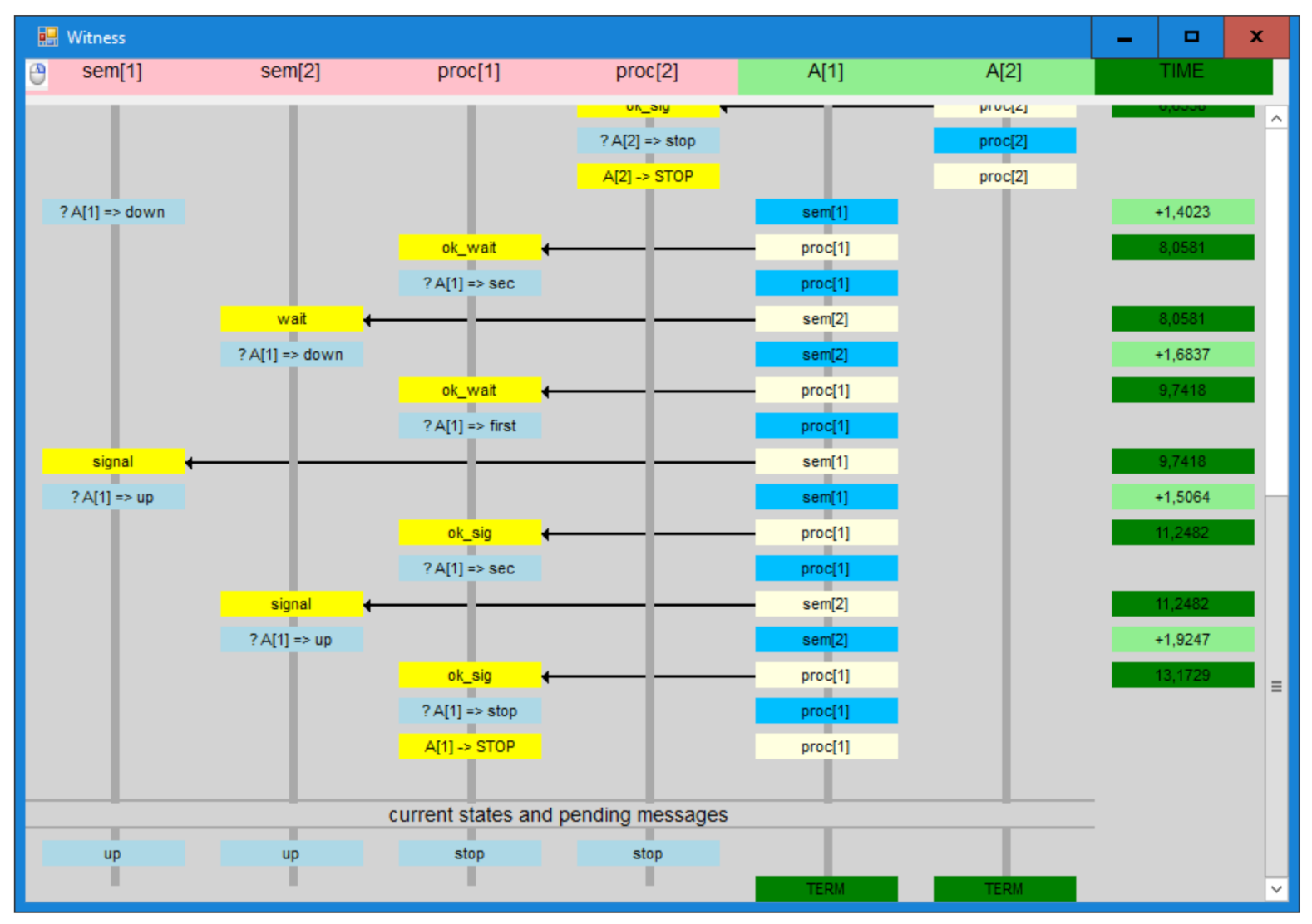
7.1. Simple Example—Two Semaphores

Let us consider two agents, starting from their own nodes, using two semaphores, each one on a separate node. The agents use the semaphores crosswise, i.e., agent a1 calls wait on the first, then on the second semaphore, and agent a2 calls wait on the second, then on the first semaphore. The T-IMDS code is presented in Section 4.1. A deadlock is evident because the semaphores are used crosswise (lines 25,26).

In the timed experiment, we assigned the duration ranges <0> to the actions in sem type, and (0,1) to the actions in proc type. The time constraints are given in Listing 4.

Listing 4.

6. {a1.sem.wait, sem.up} -> <0>{a1.sa1.ok_wait, sem.down}

…

15. {Ag.proc.start, proc.initial} -> (0,1){Ag.sem[1].wait, proc.first},

…

The channels have 0 delay.

The deadlock appears for the timed system, as before. Figure 8 presents an example of the system trace. It is a sequence diagram of the node operation, with global time values on the right (yellow). Other timeless verification examples can be found in [46,47].

If we lengthen the duration of the actions in proc[1] node (the action preceded by an index ?1), as below, the deadlock disappears, because the agent A[2] manages to perform wait operations on both semaphores before the agent A[1] can perform its first wait operation. The time constraint is given in Listing 5.

Listing 5.

15.?1{Ag.proc.start, proc.initial} -> (8,9) {Ag.sem[1].wait, proc.first}

Figure 9 shows a final part of the witness of both agents inevitable termination.

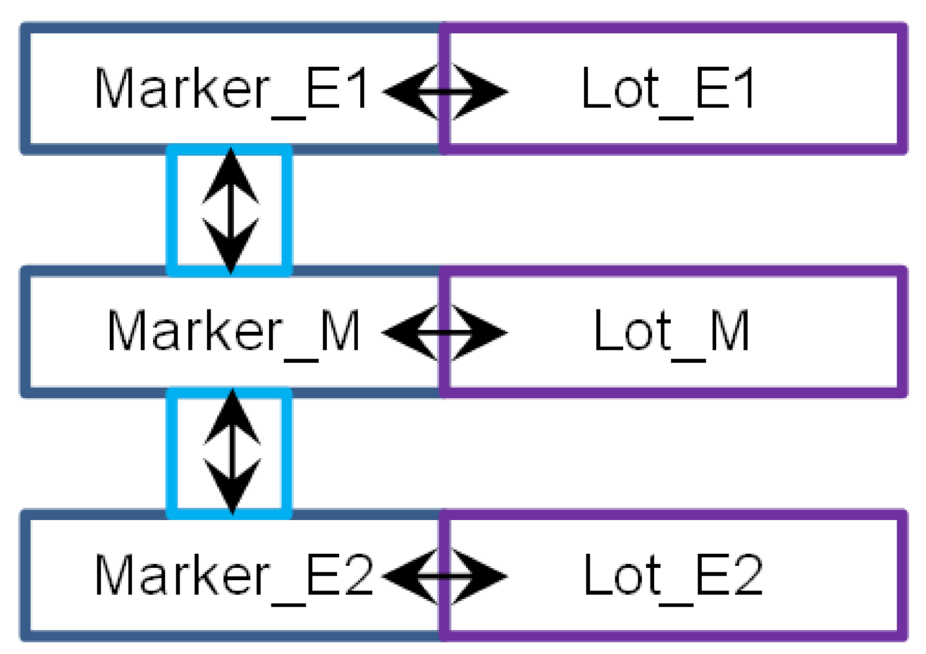
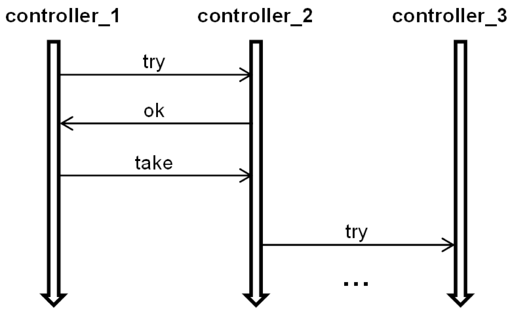
7.2. Practical Example: Automated Vehicle Guidance System

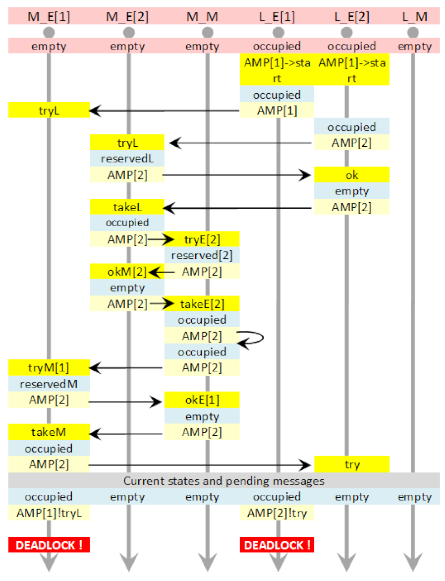
7.2.1. Timeless Verification

An automatic vehicle guidance system (AVGS) is an example of a distributed system for verification. The timeless version of the system and its verification is described by Czejdo et al. [48]. The system, depicted in Figure 6, is made up of road markers and parking lots that communicate to guide autonomous moving platforms (AMPs) from Lot_E1 to Lot_E2, and vice versa. In Marker_M, an apparent conflict can be resolved by utilizing Lot_M in a staggered arrangement. The controllers of lots and markers are represented by six nodes (Figure 10), with a protocol for requesting and granting the road segments maintained by the controllers (Figure 11). Of course, if controller_2’s road segment is occupied, the ok message may be delayed. MarkerM has a more sophisticated approach, because it allows for overtaking. The system is described from the perspective of communicating controllers in the node view. The AVGS code is shown in IMDS source notation in the node view. Node names are shortened to L_E[2], L_M, M_E[2] and M_M. The source code is given in Listing 6.

Listing 6.

1.system AVGS;

2.server: M_E(agents AMP[2];servers M_M,L_E),

3.services {tryM[2],tryL,okM[2],okL,takeM,takeL},

4. //M—going from M_M, L—going from L_E,

5. //try—test access, ok—accept, take—enter

6.states {empty,reservedM,reservedL,occupied},

7.actions {

8.<i=1..2> {AMP[i].M_E.tryL, M_E.empty} ->

<0>{AMP[i].L_E.ok, M_E.reservedL},

9.<i=1..2> {AMP[i].M_E.takeL, M_E.reservedL} ->

<0>{AMP[i].M_M.tryE[i], M_E.occupied},

10.<i=1..2><j=1..2>{AMP[i].M_E.okM[j], M_E.occupied} ->

(1,10){AMP[i].M_M.takeE[j], M_.empty},

11.<i=1..2><j=1..2>{AMP[i].M_E.tryM[j], M_E.empty} ->

<0>{AMP[i].M_M.okE[j], M_E.reservedM},

12.<i=1..2><j=1..2>{AMP[i].M_E.tryM[j], M_E.reservedL} ->

<0>{AMP[i].M_M.notE[j], M_E.reservedM},

13.<i=1..2><j=1..2>{AMP[i].M_E.tryM[j], M_E.occupied} ->

<0>{AMP[i].M_M.notE[j], M_E.occupied},

14.<i=1..2> {AMP[i].M_E.takeM, M_E.reservedM} ->

<0>{AMP[i].L_E.try, M_E.occupied},

15.<i=1..2> {AMP[i].M_E.okL, M_E.occupied} ->

(1,10){AMP[i].L_E.take, M_E.empty},

16.};

17.server: M_M(agents AMP[2];servers M_[2],L_M),

18.services {tryE[2],tryL[2],okE[2],notE[2],okL[2],takeE[2],takeL[2],switch[2]},

19.states {empty,reservedE[2],reservedL[2],occupied},

20.actions {

21.//going to M_E1 or M_E2

22.<i=1..2><j=1..2>{AMP[i].M_M.tryE[j], M_M.empty} ->

<0>{AMP[i].M_E[j].okM[j], M_M.reservedE[j]},

23.<i=1..2><j=1..2>{AMP[i].M_M.takeE[j], M_M.reservedE[j]} ->

<0>{AMP[i].M_M.switch[3-j], M_M.occupied},

24.<i=1..2><j=1..2>{AMP[i].M_M.switch[j], M_M.occupied} ->

<0>{AMP[i].M_E[j].tryM[j], M_M.occupied},

25.<i=1..2><j=1..2>{AMP[i].M_M.okE[j], M_M.occupied} ->

(1,10){AMP[i].M_E[j].takeM, M_M.empty},

26.//on a way to M_E1 or M_E2 may go to L_E if M_Ei is occupied

27.<i=1..2><j=1..2>{AMP[i].M_M.notE[j], M_M.occupied} ->

<0>{AMP[i].lotM.try[j], M_M.occupied},

28.<i=1..2><j=1..2>{AMP[i].M_M.okL[j], M_M.occupied} ->

(1,10){AMP[i].L_M.take[j], M_M.empty},

29.// from M_M—going to M_E1 or M_E2

30.<i=1..2><j=1..2>{AMP[i].M_M.tryL[j], M_M.empty} ->

<0>{AMP[i].L_M.ok[j], M_M.reservedL[j]},

31.<i=1..2><j=1..2>{AMP[i].M_M.takeL[j], M_M.reservedL[j]} ->

<0>{AMP[i].M_E[j].tryM[j], M_M.occupied},

32.<i=1..2><j=1..2>{AMP[i].M_M.okE[j], M_M.occupied} ->

(1,10){AMP[i].M_E[j].takeM, M_M.empty},

33.};

34.server: L_E(agents AMP[2];servers M_E),

35.services {start,try,ok,take},

36.states {empty,reserved,occupied},

37.actions {

38.<i=1..2> {AMP[i].L_E.try, L_E.empty} ->

<0>{AMP[i].M_E.okL, L_E.reserved},

39.<i=1..2> {AMP[i].L_E.take, lotE.reserved} ->

<0>{L_E.occupied},

40.<i=1..2> {AMP[i].L_E.start, L_E.occupied} ->

<0>{AMP[i].M_E.tryL, L_E.occupied},

41.<i=1..2> {AMP[i].L_E.ok, L_E.occupied} ->

(1,10){AMP[i].M_E.takeL, M_E.empty},

42.};

43.server: L_M(agents AMP[2];servers M_M),

44.services {try[2],ok[2],take[2]},

45.states {empty,reserved[2],occupied[2]},

46.actions {

47.<i=1..N><j=1..2>{AMP[i].L_M.try[j], L_M.empty} ->

<0>{AMP[i].M_M.okL[j], L_M.reserved[j]},

48.<i=1..N><j=1..2>{AMP[i].L_M.take[j], L_M.reserved[j]} ->

<0>{AMP[i].M_M.tryL[j], L_M.occupied[j]},

49.<i=1..2><j=1..2>{AMP[i].L_M.ok[j], L_M.occupied[j]} ->

(1,10){AMP[i].M_M.takeL[j], L_M.empty},

50.};

51.servers M_E[2],M_M,L_E[2],L_M;

52.agents AMP[2];

53.channels {(1,10)};

54.init -> {

55.<j=1..2> M_E[j](AMP[1..2],M_M,lotE[j]).empty,

56. M_M(AMP[1..2],M_E[1,2],L_M).empty,

57.<j=1..2> lotE[j](AMP[1..2],M_E[j]).occupied,

58. L_M(AMP[1..2],M_M).empty,

59.<j=1..2> AMP[j].L_E[j].start,

60.}.

The agent view of the system shows it from the point of view of AMP vehicles. The difference is generally in the grouping actions of individual agents rather than of nodes.

The Dedan program (Supplementary Materials) performs the temporal verification. Overtaking in Marker_M is successful, but there is a possibility of deadlock when an AMP occupies Marker_E1, and the other AMP tries to drive from Lot_E1 to Marker_E1. A counterexample, showing the deadlock in the node view, representing the cooperation of segment controllers, is presented in Figure 12. The counterexample is represented by a chart that resembles a sequence diagram. The upper part shows the initial states of all nodes on a pink background and the sequences of states and messages that lead to an erroneous situation in a given process (agent names on a green background occur in the agent view). The heading shows the names of the nodes on a pink background (agent names on a green background occur in the agent view). A state identifier is displayed with a light blue background. The agent responsible for entering the specified state is depicted on a dark blue background. When sending a message, the agent identifier is displayed on a light yellow background; while receiving a message, the service name is displayed on a yellow background. The last section displays the final deadlock configuration, including node states and pending messages.

In the timelines of individual nodes, messages from the various agents interleave. The counterexample can be displayed in the agent view, in which timelines of individual agents are shown. This form of counterexample, showing the behavior of individual AMPs, is presented in [48].

7.2.2. Timed Verification

The time of message passing and the time of road segment occupation are undefined in the timeless system. T-IMDS allows observing the behavior with a specified duration of actions and communication delays. Time constraints applied in the T-IMDS variant are:

• Time of movement between segments (issuing the take message) is between 1 and 10.
• The channel delay is assumed (1,10).

Setting constraints (1,10) yields the ‘nearly no restrictions’ paradigm, which is comparable to a timeless system.

Such time limits being imposed on the AVGS system result in the deadlock presented in Figure 12, as in the timeless system. However, the shorter time constraints (4,5) for taking a segment and (0,1) for channel delay model the simultaneous movement of the two AMPs, which begin practically synchronously from Lot_E1 and Lot_E2. In this case, the deadlock is broken: the AMPs use Lot_M to evade in Marker_M, but no evasive necessity occurs in Marker_E1 and Marker_E2 (time constraints do not allow the AMPs to come into a conflict in edge markers). We present the final fragment of the witness of the modified system, with shortened time constraints, in Figure 13.

8. Conclusions

This article presents the IMDS formalism and the Dedan verification environment. They support the modeling of systems using asynchronous communication of autonomous elements, which is natural in distributed environments. The node view and the agent view of the verified system can be observed, which highlight different aspects of distributed system behavior. The node view refers to the client–server model of distributed systems. In contrast, the agent view is similar to the remote procedure call model [5] (however, it is generally unnecessary for the agent process to return to the calling node in IMDS). Deadlocks can be found in both views, showing counterexamples and witnesses from the perspective of communicating nodes or agents traveling between the nodes and changing the nodes’ states.

Universal temporal formulas, unrelated to the structure of a given system, allow finding deadlocks without any knowledge of temporal logic and model checking. The location of deadlocks and distributed termination checking is performed in ‘push the button’ style.

The conversion of IMDS systems to timed automata allows the possibility of verification with real-time constraints. This is suitable for real distributed systems, where communication protocols and time-dependent behavior (such as streaming, monitoring, games) require taking time into account. Both communication delays and the time duration of nodes’ and agents’ actions can be modeled.

Verification of an existing system with the actual values of time constraints can determine if a deadlock is possible. The deadlock reveals, for example, a traffic jam. On the other hand, the threshold values of time constraints (lower and upper bounds) that cause a deadlock can be identified in a series of experiments.

Important cases include embedded systems controlling mechanical or chemical equipment, in which the system behavior depends on the time of real-world phenomena and activities. An example of such a system is presented in this article, in which time delays in controllers’ communication and the time duration of AMPs moving through road segments are modeled. IMDS and Dedan may be used for the ‘rapid prototyping’ of distributed controllers, in which sub-controllers coordinate their behavior by simple protocols; following the internet of things (IoT [49]) paradigm. We have recently started a project of train management, where the balise placement is planned (track equipment), and we estimated the maximum velocity at which the driver is safe in order to notice and acknowledge the messages coming from the balises. All elements of the system (the train, balises, and driver) act asynchronously, with their own timing constraints. Verification can be carried out for various values of time constraints.

The model is not free from limitations. The most important limitation is that distributed computations are performed by the agents, and messages are the carriers of agents. This prohibits communication in broadcast style. Multicast communication can be achieved using a set of ‘sleeping’ agents, which come into operation for multicasting. We used this technique in the verification of BPMN (business process model and notation [50]) processes [51].

The Dedan is based on explicit state–space representation, allowing for the verification of small and medium systems. Large systems are exported from Dedan to Uppaal for their verification, and the semantics of both representations are equal.

The Dedan environment has been effectively employed in the Warsaw University of Technology’s Institute of Computer Science’s operating systems laboratory. The students verify their synchronization solutions during classes.

References

- Daszczuk, W.B. Communication and Resource Deadlock Analysis using IMDS Formalism and Model Checking. Comput. J. 2017, 60, 729–750. [Google Scholar] [CrossRef]
- Daszczuk, W.B. Specification and Verification in Integrated Model of Distributed Systems (IMDS). Computers 2018, 7, 65. [Google Scholar] [CrossRef]
- Holzmann, G.J. Tutorial: Proving properties of concurrent systems with SPIN. In Proceedings of the 6th International Conference on Concurrency Theory, CONCUR’95, Philadelphia, PA, USA, 21–24 August 1995; Springer: Berlin/Heidelberg, Germany, 1995; pp. 453–455. [Google Scholar] [CrossRef]
- Zielonka, W. Notes on finite asynchronous automata. RAIRO-Theor. Inform. Appl. 1987, 21, 99–135. [Google Scholar] [CrossRef]
- Jia, W.; Zhou, W. Distributed Network Systems. From Concepts to Implementations; Springer: Berlin/Heidelberg, Germany, 2005; Volume 15. [Google Scholar] [CrossRef]
- Clarke, E.M.; Grumberg, O.; Peled, D.A. Model Checking; MIT Press: Cambridge, MA, USA, 1999. [Google Scholar]
- Kern, C.; Greenstreet, M.R. Formal verification in hardware design: A survey. ACM Trans. Des. Autom. Electron. Syst. 1999, 4, 123–193. [Google Scholar] [CrossRef]
- Inverso, O.; Nguyen, T.L.; Fischer, B.; La Torre, S.; Parlato, G. Lazy-CSeq: A Context-Bounded Model Checking Tool for Multi-threaded C-Programs. In Proceedings of the 30th IEEE/ACM International Conference on Automated Software Engineering (ASE), Lincoln, NE, USA, 9–13 November 2015; IEEE: New York, NY, USA, 2015; pp. 807–812. [Google Scholar] [CrossRef]
- Kaveh, N. Using Model Checking to Detect Deadlocks in Distributed Object Systems. In Proceedings of the 2nd International Workshop on Distributed Objects, Davis, CA, USA, 2–3 November 2000; Emmerich, W., Tai, S., Eds.; Springer: Berlin/Heidelberg, Germany, 2001; Volume 1999, pp. 116–128. [Google Scholar] [CrossRef]
- Arcaini, P.; Gargantini, A.; Riccobene, E. AsmetaSMV: A Model Checker for AsmetaL Models–Tutorial; Report, Università degli Studi di Milano, Dipartimento di Tecnologie dell’Informazione; 2009; Available online: https://air.unimi.it/retrieve/handle/2434/69105/96882/Tutorial_AsmetaSMV.pdf (accessed on 30 January 2022).
- Yang, Y.; Chen, X.; Gopalakrishnan, G. Inspect: A Runtime Model Checker for Multithreaded C Programs; Report UUCS-08-004; University of Utah: Salt Lake City, UT, USA, 2008; Available online: http://www.cs.utah.edu/docs/techreports/2008/pdf/UUCS-08-004.pdf (accessed on 1 February 2022).
- Podelski, A.; Rybalchenko, A. Software Model Checking of Liveness Properties via Transition Invariants; Research Report MPI–I–2003–2–00; Max Planck Institut für Informatik: Saarbrücken, Germany, 2003; Available online: https://pure.mpg.de/pubman/faces/ViewItemOverviewPage.jsp?itemId=item_1819221 (accessed on 30 January 2022).
- Behrmann, G.; David, A.; Larsen, K.G.; Pettersson, P.; Yi, W. Developing UPPAAL over 15 years. Softw. Pract. Exp. 2011, 41, 133–142. [Google Scholar] [CrossRef]
- Behrmann, G.; David, A.; Larsen, K.G. A Tutorial on Uppaal 4.0; Aalborg University: Aalborg, Denmark, 2006; Available online: http://www.it.uu.se/research/group/darts/papers/texts/new-tutorial.pdf (accessed on 30 January 2022).
- Daszczuk, W.B. Evaluation of temporal formulas based on “Checking By Spheres”. In Proceedings of the Euromicro Symposium on Digital Systems Design, Warsaw, Poland, 4–6 September 2001; IEEE: New York, NY, USA, 2001; pp. 158–164. [Google Scholar] [CrossRef]
- Holzmann, G.J. The model checker SPIN. IEEE Trans. Softw. Eng. 1997, 23, 279–295. [Google Scholar] [CrossRef]
- Cimatti, A.; Clarke, E.M.; Giunchiglia, F.; Roveri, M. NUSMV: A new symbolic model checker. Int. J. Softw. Tools Technol. Transf. 2000, 2, 410–425. [Google Scholar] [CrossRef]
- Alur, R.; Dill, D.L. A theory of timed automata. Theor. Comput. Sci. 1994, 126, 183–235. [Google Scholar] [CrossRef]
- Bérard, B.; Cassez, F.; Haddad, S.; Lime, D.; Roux, O.H. Comparison of the Expressiveness of Timed Automata and Time Petri Nets. In Proceedings of the Third International Conference, FORMATS 2005, Uppsala, Sweden, 26–28 September 2005; Springer: Berlin/Heidelberg, Germany, 2005; pp. 211–225. [Google Scholar] [CrossRef]
- Popescu, C.; Martinez Lastra, J.L. Formal Methods in Factory Automation. In Factory Automation; Silvestre-Blanes, J., Ed.; InTech: Rijeka, Croatia, 2010; pp. 463–475. [Google Scholar] [CrossRef]
- Daszczuk, W.B. Threefold Analysis of Distributed Systems: IMDS, Petri Net and Distributed Automata DA3. In Proceedings of the 37th IEEE Software Engineering Workshop, Federated Conference on Computer Science and Information Systems, FEDCSIS’17, Prague, Czech Republic, 3–6 September 2017; IEEE Computer Society Press: New York, NY, USA, 2017; pp. 377–386. [Google Scholar] [CrossRef]
- Daszczuk, W.B. Siphon-based deadlock detection in Integrated Model of Distributed Systems (IMDS). In Proceedings of the Federated Conference on Computer Science and Information Systems, 3rd Workshop on Constraint Programming and Operation Research Applications (CPORA’18), Poznań, Poland, 9–12 September 2018; IEEE: New York, NY, USA, 2018; pp. 425–435. [Google Scholar] [CrossRef]
- Bérard, B. An Introduction to Timed Automata. In Control of Discrete-Event Systems; Springer: Berlin/Heidelberg, Germany, 2013; pp. 169–187. [Google Scholar] [CrossRef]
- Glabbeek, R.J.; Goltz, U. Equivalences and refinement. In Proceedings of the LITP Spring School on Theoretical Computer Science La Roche Posay, France, 23–27 April 1990; Springer: Berlin/Heidelberg, Germany, 1990; pp. 309–333. [Google Scholar] [CrossRef]
- Lime, D.; Roux, O.H. Model Checking of Time Petri Nets Using the State Class Timed Automaton. Discret. Event Dyn. Syst. 2006, 16, 179–205. [Google Scholar] [CrossRef]
- Cassez, F.; Roux, O.H. Structural translation from Time Petri Nets to Timed Automata. J. Syst. Softw. 2006, 79, 1456–1468. [Google Scholar] [CrossRef]
- Henzinger, T.A.; Ho, P.-H.; Wong-Toi, H. A user guide to HyTech. In Proceedings of the TACAS 95: International Workshop on Tools and Algorithms for the Construction and Analysis of Systems, Aarhus, Denmark, 19–20 May 1995; Springer: Berlin/Heidelberg, Germany, 1995; pp. 41–71. [Google Scholar] [CrossRef]
- André, É.; Fribourg, L.; Kühne, U.; Soulat, R. IMITATOR 2.5: A Tool for Analyzing Robustness in Scheduling Problems. In Proceedings of the FM 2012: International Symposium on Formal Methods, Paris, France, 27–31 August 2012; Springer: Berlin/Heidelberg, Germany, 2012; pp. 33–36. [Google Scholar] [CrossRef]
- Laroussinie, F.; Markey, N.; Schnoebelen, P. Efficient timed model checking for discrete-time systems. Theor. Comput. Sci. 2006, 353, 249–271. [Google Scholar] [CrossRef]
- Krystosik, A.; Turlej, D. Emlan: A Language for model checking of embedded systems software. IFAC Proc. Vol. 2006, 39, 126–131. [Google Scholar] [CrossRef]
- Emerson, E.A.; Mok, A.K.; Sistla, A.P.; Srinivasan, J. Quantitative temporal reasoning. Real-Time Syst. 1992, 4, 331–352. [Google Scholar] [CrossRef]
- Gluchowski, P. Languages of CTL and RTCTL Calculi in Real-Time Analysis of a System Described by a Fault Tree with Time Dependencies. In Proceedings of the 2009 Fourth International Conference on Dependability of Computer Systems, DepCoS-RELCOMEX’09, Brunów, Poland, 30 June–2 July 2009; IEEE: New York, NY, USA, 2009; pp. 33–41. [Google Scholar] [CrossRef]
- Frossl, J.; Gerlach, J.; Kropf, T. An efficient algorithm for real-time symbolic model checking. In Proceedings of the ED&TC European Design and Test Conference, Paris, France, 11–14 March 1996; IEEE Computer Society Press: New York, NY, USA, 1996; pp. 15–20. [Google Scholar] [CrossRef]
- Audemard, G.; Cimatti, A.; Kornilowicz, A.; Sebastiani, R. Bounded Model Checking for Timed Systems. In Proceedings of the FORTE 2002: International Conference on Formal Techniques for Networked and Distributed Systems, Houston, TX, USA, 11–14 November 2002; Springer: Berlin/Heidelberg, Germany, 2002; pp. 243–259. [Google Scholar] [CrossRef]
- Ruf, J.; Kropf, T. Symbolic Verification and Analysis of Discrete Timed Systems. Form. Methods Syst. Des. 2003, 23, 67–108. [Google Scholar] [CrossRef]
- Winskel, G.; Nielsen, M. Models for Concurrency. Handbook of Logic in Computer Science; Oxford University Press: Oxford, UK, 1995; Volume 4. [Google Scholar]
- Bowman, H. Time and Action Lock Freedom Properties for Timed Automata. In Proceedings of the 21st International Conference on Formal Techniques for Networked and Distributed Systems, FORTE 2001, Cheju Island, Korea, 28–31 August 2001; Kluwer Academic Publishers: Boston, MA, USA, 2001; pp. 119–134. [Google Scholar] [CrossRef]
- Keller, R.M. Formal verification of parallel programs. Commun. ACM 1976, 19, 371–384. [Google Scholar] [CrossRef]
- Reniers, M.A.; Willemse, T.A.C. Folk Theorems on the Correspondence between State-Based and Event-Based Systems. In Proceedings of the 37th Conference on Current Trends in Theory and Practice of Computer Science, Nový Smokovec, Slovakia, 22–28 January 2011; Springer: Berlin/Heidelberg, Germany, 2011; Volume 6543, pp. 494–505. [Google Scholar] [CrossRef]
- Daszczuk, W.B. Graphic modeling in Distributed Autonomous and Asynchronous Automata (DA3). Softw. Syst. Model. 2021, 20, 36. [Google Scholar] [CrossRef]
- Chrobot, S. Modelling communication in distributed systems. In Proceedings of the International Conference on Parallel Computing in Electrical Engineering PARELEC 2002, Warsaw, Poland, 25 September 2002; IEEE Computer Society: New York, NY, USA, 2002; pp. 55–60. [Google Scholar] [CrossRef]
- Daszczuk, W.B.; Bielecki, M.; Michalski, J. Rybu: Imperative-style Preprocessor for Verification of Distributed Systems in the Dedan Environment. In Proceedings of the KKIO’17–Software Engineering Conference, Rzeszów, Poland, 14–16 September 2017; Polish Information Processing Society: Warshaw, Poland, 2017; pp. 135–150. [Google Scholar]
- Penczek, W.; Szreter, M.; Gerth, R.; Kuiper, R. Improving Partial Order Reductions for Universal Branching Time Properties. Fundam. Inform. 2000, 43, 245–267. [Google Scholar] [CrossRef]
- Lanese, I.; Montanari, U. Hoare vs Milner: Comparing Synchronizations in a Graphical Framework With Mobility. Electron. Notes Theor. Comput. Sci. 2006, 154, 55–72. [Google Scholar] [CrossRef][Green Version]
- May, D. Occam. ACM Sigplan Not. 1983, 18, 69–79. [Google Scholar] [CrossRef]
- Daszczuk, W.B. Asynchronous Specification of Production Cell Benchmark in Integrated Model of Distributed Systems. In Proceedings of the 23rd International Symposium on Methodologies for Intelligent Systems, ISMIS 2017, Warsaw, Poland, 26–29 June 2017; Bembenik, R., Skonieczny, L., Protaziuk, G., Kryszkiewicz, M., Rybinski, H., Eds.; Springer International Publishing: Cham, Switzerland, 2019; Volume 40, pp. 115–129. [Google Scholar] [CrossRef]
- Daszczuk, W.B. Static and Dynamic Verification of Space Systems Using Asynchronous Observer Agents. Sensors 2021, 21, 4541. [Google Scholar] [CrossRef]
- Czejdo, B.; Bhattacharya, S.; Baszun, M.; Daszczuk, W.B. Improving Resilience of Autonomous Moving Platforms by real-time analysis of their Cooperation. Autobusy-TEST 2016, 17, 1294–1301. Available online: http://yadda.icm.edu.pl/baztech/element/bwmeta1.element.baztech-6ab8a90d-13a7-429b-9ecd33cce2801f6f/c/10_L_CZEJDO_BHATTACHARYA_BASZUN_DASZCZUK.pdf (accessed on 30 January 2022).
- Lee, G.M.; Crespi, N.; Choi, J.K.; Boussard, M. Internet of Things. In Evolution of Telecommunication Services; Springer: Berlin/Heidelberg, Germany, 2013; pp. 257–282. [Google Scholar] [CrossRef]
- Grosskopf, A.; Decker, G.; Weske, M. The Process: Business Process Modeling Using BPMN; Meghan-Kiffer Press: Tampa, FL, USA, 2018; p. 182. ISBN 9780929652269. [Google Scholar]
- Jałowiec, J. Translation of Business Process Model and Notation into Integrated Model of Distributed Systems. Available online: https://repo.pw.edu.pl/info/bachelor/WUT31de757656da422c87be61e7ede00630/?r=diploma&tab=&lang=pl (accessed on 30 January 2022).
Publisher’s Note: MDPI stays neutral with regard to jurisdictional claims in published maps and institutional affiliations. |
© 2022 by the author. Licensee MDPI, Basel, Switzerland. This article is an open access article distributed under the terms and conditions of the Creative Commons Attribution (CC BY) license (https://creativecommons.org/licenses/by/4.0/).
Share and Cite
Daszczuk, W.B. Modeling and Verification of Asynchronous Systems Using Timed Integrated Model of Distributed Systems. Sensors 2022, 22, 1157. https://doi.org/10.3390/s22031157
Daszczuk WB. Modeling and Verification of Asynchronous Systems Using Timed Integrated Model of Distributed Systems. Sensors. 2022; 22(3):1157. https://doi.org/10.3390/s22031157
Chicago/Turabian StyleDaszczuk, Wiktor B. 2022. "Modeling and Verification of Asynchronous Systems Using Timed Integrated Model of Distributed Systems" Sensors 22, no. 3: 1157. https://doi.org/10.3390/s22031157
APA StyleDaszczuk, W. B. (2022). Modeling and Verification of Asynchronous Systems Using Timed Integrated Model of Distributed Systems. Sensors, 22(3), 1157. https://doi.org/10.3390/s22031157