
A Machine-Learning Model for Lung Age Forecasting by Analyzing Exhalations

 , , , , , and
Abstract
:1. Introduction
2. Methods
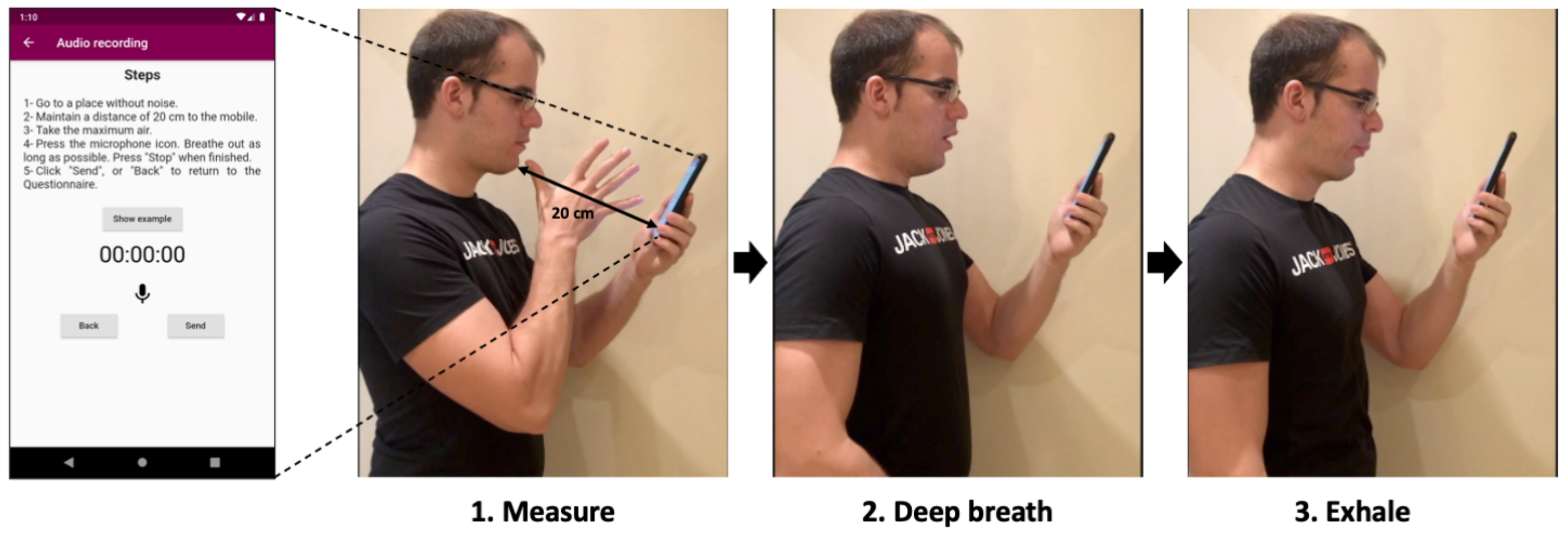
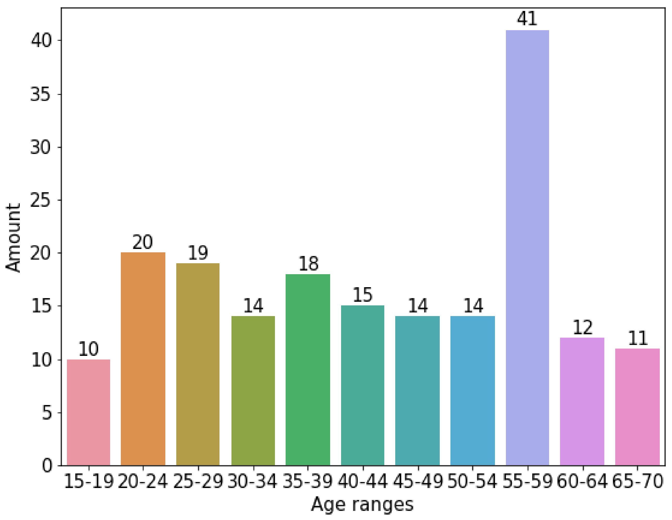
2.1. Corpus
2.2. Features
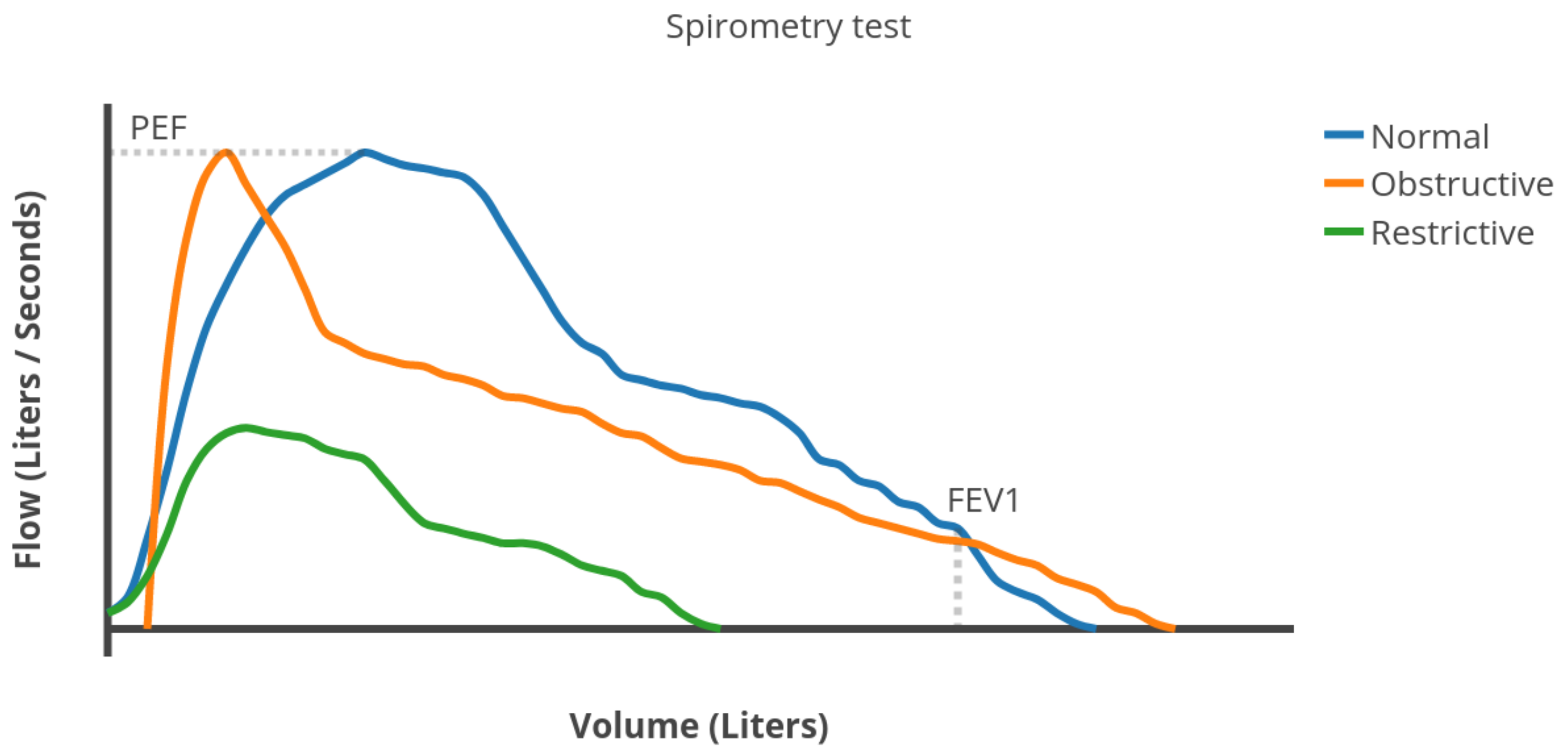
2.2.1. Spimoreter-Like Features
- Forced Vital Capacity (FVC): the total volume of air expelled during the expiration.
- Forced Expiratory Volume in one second (FEV1): the volume of air expelled in the first second of expiration.
- Peak Expiratory Flow (PEF): the maximum expiratory flow rate reached during the exhalation.
- Total_dec: The summation of all the decibels of the audio over all frequencies as an absolute value. This is an approximation to FVC.
- Total_dec_1st_sec. The sum of all the decibels during the first second of the audio over all frequencies as an absolute value. This is an approximation to FEV1.
- Max_peak. The maximum peak of decibels from all the audio and frequencies. This is an approximation to PEF.
2.2.2. Time-Frequency Features
- E_Bn1…E_Bn7: average of the instantaneous spectral energy E(t) (Equation (2)) of each sample, for each 7-bands.where and are the lower and upper frequencies of each band.
- f_Cres1…f_Cres7: average of the Instantaneous Frequency Peak, (Equation (3)), for each 7-bands.
- f_Med1…f_Med7: average of the instantaneous frequency (Equation (4)), for each 7-bands.
- IE_Bn1…IE_Bn7: average of the spectral information, (Equation (5)), for each 7-bands.
- K: Kurtosis (Equation (9)).
- The joint time-frequency moments for and (momC11), and (momC77) and and (momC15).
- The same joint moments of the marginal signals of instantaneous power and spectral density (momM11, momM77 and momM15) were also considered.
2.3. Prediction Models
2.4. Performance Metrics
- Accuracy (Equation (10)). The ratio between the correctly classified samples.
- Sensitivity (Equation (11)). The proportion of correctly classified positive samples compared to the total number of positive samples.
- Specificity (Equation (12)). The proportion of correctly classified negative samples compared to the total number of negative samples.
3. Results
3.1. Prescreening
3.1.1. Correlation Analysis
3.1.2. Principal Component Analysis
3.1.3. Oversampling
3.2. Group Classification
3.3. Classification Accuracy
4. Discussion
4.1. Comparison with Previous Work
4.2. Limitations
5. Conclusions
Author Contributions
Funding
Institutional Review Board Statement
Informed Consent Statement
Data Availability Statement
Acknowledgments
Conflicts of Interest
Sample Availability
Abbreviations
| LDA | Linear Discrimination Analysis. |
| QDA | Quadratic Linear Analysis. |
| PCA | Principal Component Analysis |
| SMOTE | Synthetic Minority Oversampling Technique. |
| FVC | Forced Vital Capacity |
| FEV1 | Forced Expiratory Volume in one second |
| PEF | Peak Expiratory Flow |
| COPD | Chronic obstructive pulmonary disease |
| GSM | Global System for Mobile communications |
| RMSE | Root Mean Square |
| CEIM | Research Ethics Committee for Biomedical Research Projects |
| ALS | Amyotrophic lateral sclerosis |
| STFT | Short-time Fourier transform |
| WD | Wigner distribution |
| CWD | Choi–Williams distribution |
| K-NN | K-Nearest Neighbor |
| C-SVC | C-Support Vector Classification |
| RF | Random Forest |
| DT | Decision Tree |
| NB | Naïve Bayes |
| LR | Logistic Regression |
| LDA | Linear Discriminant Analysis |
| QDA | Quadratic Discriminant Analysis |
| TP | True Positive |
| FN | False Negative |
| FP | False Positive |
| TN | True negative |
References
- World Health Organization (WHO). The Top 10 Causes of Death. Available online: http://www.who.int/en/news-room/fact-sheets/detail/the-top-10-causes-of-death (accessed on 9 December 2020).
- Gibson, G.J.; Loddenkemper, R.; Lundbäck, B.; Sibille, Y. Respiratory health and disease in Europe: The new European Lung White Book. Eur. Respir. J. 2013, 42, 559–563. [Google Scholar] [CrossRef] [PubMed]
- Marques, A.; Oliveira, A.; Jácome, C. Computerized Adventitious Respiratory Sounds as Outcome Measures for Respiratory Therapy: A Systematic Review. Respir. Care 2014, 59, 765–776. [Google Scholar] [CrossRef] [PubMed] [Green Version]
- Rocha, B.M.; Filos, D.; Mendes, L.; Vogiatzis, I.; Perantoni, E.; Kaimakamis, E.; Natsiavas, P.; Jácome, C.; Marques, A.; Paiva, R.P.; et al. A Respiratory Sound Database for the Development of Automated Classification. Precision Medicine Powered by pHealth and Connected Health; Springer: Singapore, 2018; pp. 51–55. [Google Scholar]
- Reichert, S.; Gass, R.; Brandt, C.; Andrès, E. Analysis of respiratory sounds: State of the art. Clin. Med. Circ. Respir. Pulm. Med. 2008, 2, 45–58. [Google Scholar] [CrossRef] [PubMed]
- Sovijärvi, A.R.A.; Dalmasso, F.; Vanderschoot, J.; Malmberg, L.P.; Righini, G.; Stoneman, S.A.T. Definition of terms for applications of respiratory sounds. Eur. Respir. Rev. 2000, 10, 597–610. [Google Scholar]
- Brouwer, A.F.J.; Roorda, R.J.; Brand, P.L.P. Home spirometry and asthma severity in children. Eur. Respir. J. 2006, 28, 1131–1137. [Google Scholar] [CrossRef] [Green Version]
- Sevick, M.A.; Trauth, J.M.; Ling, B.S.; Anderson, R.T.; Piatt, G.A.; Kilbourne, A.M.; Goodman, R.M. Patients with Complex Chronic Diseases: Perspectives on supporting self-management. J. Gen. Intern. Med. 2007, 22, 438–444. [Google Scholar] [CrossRef] [Green Version]
- Grzincich, G.; Gagliardini, R.; Bossi, A.; Bella, S.; Cimino, G.; Cirilli, N.; Viviani, L.; Iacinti, E.; Quattrucci, S. Evaluation of a home telemonitoring service for adult patients with cystic fibrosis: A pilot study. J. Telemed. Telecare 2010, 16, 359–362. [Google Scholar] [CrossRef]
- Chu, S.; Narayanan, S.; Kuo, C.C.J. Environmental Sound Recognition With Time–Frequency Audio Features. IEEE Trans. Audio Speech Lang. Process. 2009, 17, 1142–1158. [Google Scholar] [CrossRef]
- Knudson, R.J.; Slatin, R.C.; Lebowitz, M.D.; Burrows, B. The maximal expiratory flow-volume curve. Normal standards, variability, and effects of age. Am. Rev. Respir. Dis. 1992, 46, 2139–2148. [Google Scholar] [CrossRef]
- Baken, R.J.; Orlikoff, R.F. Clinical Measurement of Speech and Voice, 2nd ed.; Singular Thomson Learning: San Diego, CA, USA, 2000. [Google Scholar]
- Kassem, A.; Hamad, M.; El Moucary, C. A smart spirometry device for asthma diagnosis. In Proceedings of the Annual International Conference of the IEEE Engineering in Medicine and Biology Society, EMBS, Milan, Italy, 25–29 August 2015; pp. 1629–1632. [Google Scholar] [CrossRef]
- Larson, E.C.; Goel, M.; Boriello, G.; Heltshe, S.; Rosenfeld, M.; Patel, S.N. SpiroSmart: Using a Microphone to Measure Lung Function on a Mobile Phone. In Proceedings of the 2012 ACM Conference on Ubiquitous Computing, 5–8 September 2012; ACM: New York, NY, USA, 2012; pp. 280–289. [Google Scholar] [CrossRef]
- Goel, M.; Saba, E.; Stiber, M.; Whitmire, E.; Fromm, J.; Larson, E.C.; Borriello, G.; Patel, S.N. SpiroCall: Measuring lung function over a phone call. In Proceedings of the Conference on Human Factors in Computing Systems, San Jose, CA, USA, 7–12 May 2016; pp. 5675–5685. [Google Scholar] [CrossRef] [Green Version]
- Zubaydi, F.; Sagahyroon, A.; Aloul, F.; Mir, H. MobSpiro: Mobile based spirometry for detecting COPD. In Proceedings of the 2017 IEEE 7th Annual Computing and Communication Workshop and Conference, CCWC 2017, Las Vegas, NV, USA, 9–11 January 2017. [Google Scholar] [CrossRef]
- Viswanath, V.; Garrison, J.; Patel, S. SpiroConfidence: Determining the Validity of Smartphone Based Spirometry Using Machine Learning. In Proceedings of the 2018 40th Annual International Conference of the IEEE Engineering in Medicine and Biology Society (EMBC), Honolulu, HI, USA, 17–21 July 2018; pp. 5499–5502. [Google Scholar]
- Deane, K.; Stevermer, J.J.; Hickner, J. Help smokers quit: Tell them their “lung age”. J. Family Pract. 2008, 57, 584–586. [Google Scholar]
- Carbonneau, M.A.; Gagnon, G.; Sabourin, R.; Dubois, J. Recognition of blowing sound types for real-time implementation in mobile devices. In Proceedings of the 2013 IEEE 11th International New Circuits and Systems Conference, NEWCAS 2013, Paris, France, 16–19 June 2013. [Google Scholar] [CrossRef]
- Miller, M.R.; Hankinson, J.; Brusasco, V.; Burgos, F.; Casaburi, R.; Coates, A.; Crapo, R.; Enright, P.; van der Grinten, C.P.M.; Gustafsson, P.; et al. Standardisation of spirometry. Eur. Respir. J. 2005, 26, 319–338. [Google Scholar] [CrossRef] [PubMed] [Green Version]
- McFee, B.; Raffel, C.; Liang, D.; Ellis, D.P.W.; McVicar, M.; Battenberg, E.; Nieto, O. Librosa: Audio and music signal analysis in python. In Proceedings of the 14th Python in Science Conference, Austin, TX, USA, 6–12 July 2015; pp. 18–25. [Google Scholar]
- Tena, A.; Clarià, F.; Solsona, F. Automated detection of COVID-19 cough. Biomed. Signal Process. Control 2022, 71, 103175. [Google Scholar] [CrossRef] [PubMed]
- Pedregosa, F.; Varoquaux, G.; Gramfort, A.; Michel, V.; Thirion, B.; Grisel, O.; Blondel, M.; Prettenhofer, P.; Weiss, R.; Dubourg, V.; et al. Scikit-Learn: Machine Learning in Python. J. Mach. Learn. Res. 2011, 12, 2825–2830. [Google Scholar]
- Altman, N.S. An Introduction to Kernel and Nearest-Neighbor Nonparametric Regression. Am. Stat. 1992, 46, 175–185. [Google Scholar]
- Novakovic, J.; Veljovic, A. C-Support Vector Classification: Selection of kernel and parameters in medical diagnosis. In Proceedings of the 2011 IEEE 9th International Symposium on Intelligent Systems and Informatics, Subotica, Serbia, 8–10 September 2011; pp. 465–470. [Google Scholar] [CrossRef]
- Cutler, A.; Cutler, D.R.; Stevens, J.R. Random Forests; Springer: Boston, MA, USA, 2012; pp. 157–175. [Google Scholar] [CrossRef]
- Nowozin, S.; Rother, C.; Bagon, S.; Sharp, T.; Yao, B.; Kohli, P. Decision tree fields. In Proceedings of the IEEE International Conference on Computer Vision, Barcelona, Spain, 6–13 November 2011; pp. 1668–1675. [Google Scholar] [CrossRef]
- Rish, I. An Empirical Study of the Naive Bayes Classifier. In Proceedings of the IJCAI 2001 Work Empir Methods Artif Intell, Seattle, WA, USA, 3–10 August 2001. [Google Scholar]
- Lemon, S.C.; Roy, J.; Clark, M.A.; Friedmann, P.D.; Rakowski, W. Classification and regression tree analysis in public health: Methodological review and comparison with logistic regression. Ann. Behav. Med. 2003, 26, 172–181. [Google Scholar] [CrossRef] [PubMed]
- Izenman, A.J. Linear Discriminant Analysis; Springer: New York, NY, USA, 2013; pp. 237–280. [Google Scholar] [CrossRef]
- Tharwat, A. Linear vs. quadratic discriminant analysis classifier: A tutorial. Int. J. Appl. Pattern Recognit. 2016, 3, 145–180. [Google Scholar] [CrossRef]
- Tharwat, A. Classification assessment methods. Appl. Comput. Inform. 2021, 17, 168–192. [Google Scholar] [CrossRef]
- Hothorn, T.; Leisch, F.; Zeileis, A.; Hornik, K. The Design and Analysis of Benchmark Experiments. J. Comput. Graph. Stat. 2005, 14, 675–699. [Google Scholar] [CrossRef] [Green Version]
- Mckinney, W. pandas: A Foundational Python Library for Data Analysis and Statistics. Python High Perform. Sci. Comput. 2011, 14, 1–9. [Google Scholar]
- Chawla, N.; Bowyer, K.; Hall, L.; Kegelmeyer, W. SMOTE: Synthetic Minority Over-sampling Technique. J. Artif. Intell. Res. (JAIR) 2002, 16, 321–357. [Google Scholar] [CrossRef]
- Toda, R.; Hoshino, T.; Kawayama, T.; Imaoka, H.; Sakazaki, Y.; Tsuda, T.; Takada, S.; Kinoshita, M.; Iwanaga, T.; Aizawa, H. Validation of “lung age” measured by spirometry and handy electronic FEV1/FEV6 meter in pulmonary diseases. Intern. Med. 2009, 48, 513–521. [Google Scholar] [CrossRef] [PubMed] [Green Version]


| Classifiers | No SMOTE | SMOTE | ||||
|---|---|---|---|---|---|---|
| Acc. | Sen. | Spe. | Acc. | Sen. | Spe. | |
| K-NN | 4.26% | 10.91% | 90.07% | 50.44% | 56.26% | 95.50% |
| C-SVC | 25.53% | 9.09% | 90.91% | 4.43% | 9.09% | 90.91% |
| DT | 17.02% | 19.78% | 91.36% | 60.18% | 64.75% | 95.99% |
| RF | 12.77% | 6.15% | 90.57% | 74.34% | 77.89% | 97.45% |
| NB | 10.64% | 16.00% | 91.07% | 42.48% | 47.11% | 94.24% |
| LR | 14.89% | 6.91% | 90.64% | 38.05% | 43.87% | 93.91% |
| LDA | 6.38% | 3.90% | 90.33% | 50.44% | 53.86% | 95.05% |
| QDA | 12.77% | 8.20% | 90.97% | 94.69% | 94.45% | 99.45% |
| Classifiers | Men | Women | ||||
|---|---|---|---|---|---|---|
| Acc. | Sen. | Spe. | Acc. | Sen. | Spe. | |
| K-NN | 60.00% | 59.00% | 95.48% | 66.67% | 67.05% | 96.63% |
| C-SVC | 20.00% | 35.00% | 91.52% | 4.17% | 9.09% | 90.91% |
| DT | 45.71% | 48.00% | 93.85% | 65.28% | 64.77% | 96.57% |
| RF | 62.86% | 63.50% | 95.84% | 77.78% | 79.48% | 97.80% |
| NB | 57.14% | 59.00% | 95.21% | 54.17% | 57.88% | 95.37% |
| LR | 48.57% | 49.50% | 94.24% | 47.22% | 53.33% | 94.77% |
| LDA | 57.14% | 57.00% | 95.22% | 66.67% | 68.34% | 96.67% |
| QDA | 74.29% | 74.67% | 97.16% | 91.67% | 92.73% | 99.16% |
Publisher’s Note: MDPI stays neutral with regard to jurisdictional claims in published maps and institutional affiliations. |
© 2022 by the authors. Licensee MDPI, Basel, Switzerland. This article is an open access article distributed under the terms and conditions of the Creative Commons Attribution (CC BY) license (https://creativecommons.org/licenses/by/4.0/).
Share and Cite
Pifarré, M.; Tena, A.; Clarià, F.; Solsona, F.; Vilaplana, J.; Benavides, A.; Mas, L.; Abella, F. A Machine-Learning Model for Lung Age Forecasting by Analyzing Exhalations. Sensors 2022, 22, 1106. https://doi.org/10.3390/s22031106
Pifarré M, Tena A, Clarià F, Solsona F, Vilaplana J, Benavides A, Mas L, Abella F. A Machine-Learning Model for Lung Age Forecasting by Analyzing Exhalations. Sensors. 2022; 22(3):1106. https://doi.org/10.3390/s22031106
Chicago/Turabian StylePifarré, Marc, Alberto Tena, Francisco Clarià, Francesc Solsona, Jordi Vilaplana, Arnau Benavides, Lluis Mas, and Francesc Abella. 2022. "A Machine-Learning Model for Lung Age Forecasting by Analyzing Exhalations" Sensors 22, no. 3: 1106. https://doi.org/10.3390/s22031106
APA StylePifarré, M., Tena, A., Clarià, F., Solsona, F., Vilaplana, J., Benavides, A., Mas, L., & Abella, F. (2022). A Machine-Learning Model for Lung Age Forecasting by Analyzing Exhalations. Sensors, 22(3), 1106. https://doi.org/10.3390/s22031106