
Multi-Modal Song Mood Detection with Deep Learning †


Abstract
:1. Introduction
2. From Audio and Lyrics to Mood
2.1. From Audio to Mood
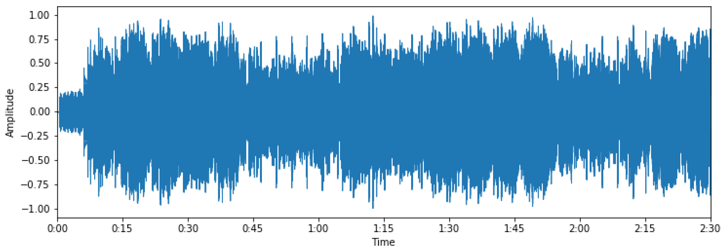
- Spectrogram comes from the Short-Time Fourier Transform of a signal and expresses the sinusoidal frequency and phase content of signal’s sections (windows) as they vary over time. In practice, to calculate the STFT the signal is divided into segments of equal length to which the Fourier transform is applied, highlighting thus the Fourier spectrum. The process of displaying variable spectra as a function of time is known as a Spectrogram.In the case of continuous time, the function we want to transform, let , is multiplied by a window function which is non-zero for a short time. Usually for the window function, , the Hann or Gaussian type windows are used. The Fourier transform, for STFT, is calculated as the window slides up in the signal and mathematically calculated from Equation (1).
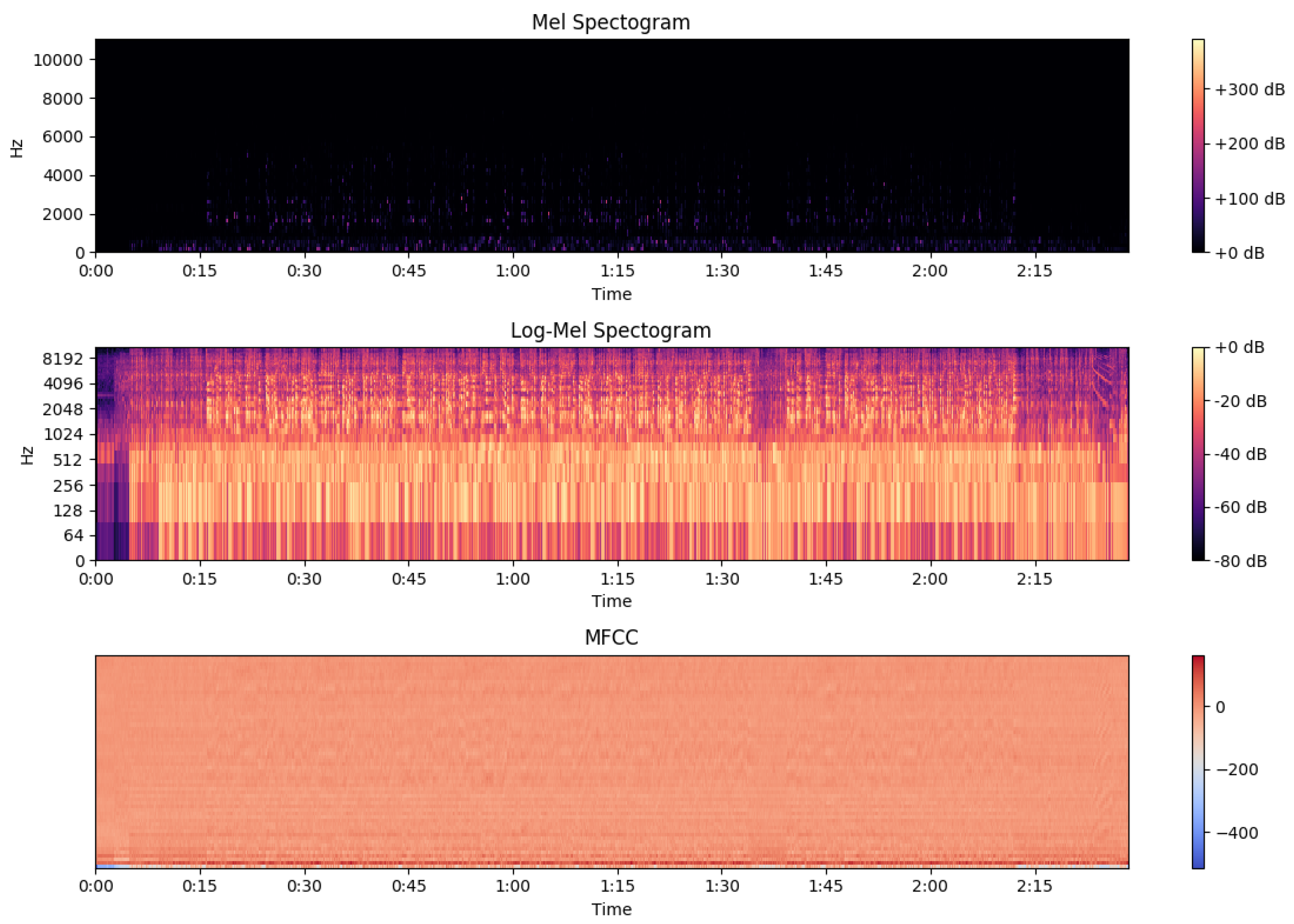
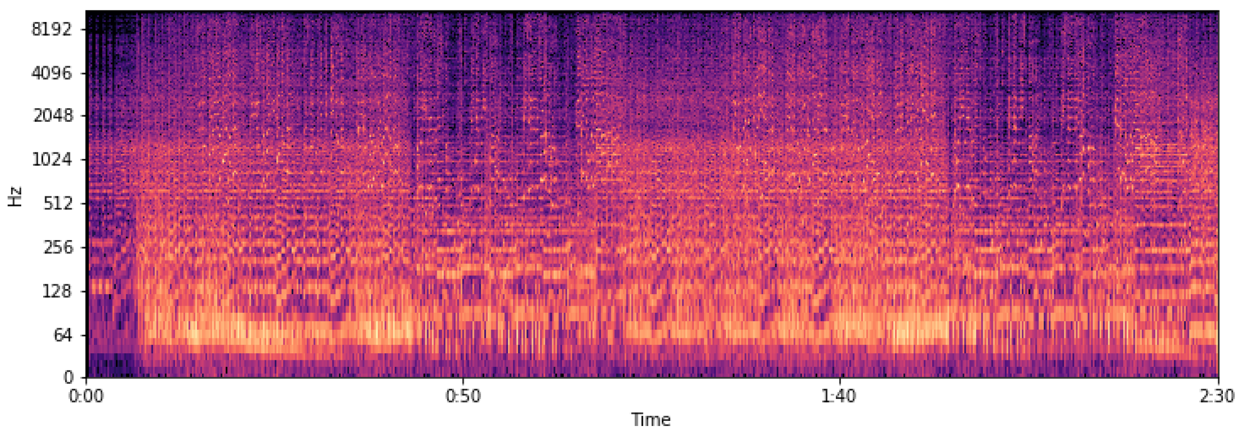
- Mel Spectrogram is almost like Spectrogram, with the only difference that frequencies are transformed to the Mel scale. Mel scale is a scale of pitches, able to mimic the auditory system of a human.Mel filters mimic the response of the human auditory system with better performance than linear frequency bands. Essentially, the term Mel refers to a pitch scale created by experiments on listeners for the purpose of recognizing tonal changes perceived by the human ear. The rendering of the name is due to Stevens, Volkmann, Newman [24] and comes from the word melody (melody).
- Log-Mel Spectrogram is the Mel Spectrogram with a logarithmic transformation on the frequency axis.
- Mel-Frequency Cepstral Coefficients (MFCCs) comes from the Log-Mel Spectrogram with a linear cosine transformation.where is the logarithmic energy of m-th Log-Mel Spectrogram and c is the index of the cepstral coefficient.
- Chroma features, or pitch class profiles, are strongly correlated with music harmony and are widely used in music information retrieval tasks. Chroma features are not affected by changes in tonal quality (timbre) and are directly related to musical harmony. According to Müller [25], Chroma features are strong mid level features capable of retrieving important information from audio.If we assume the tonal scale used in western music (4), then it is easy to describe the matching between audio signal and chroma features. In practice, first we compute the Spectrogram of the signal and then for each window a vector is calculated , where each element represents the corresponding element in scale (4).
- Tonnetz (or centroid tonal features) [29], is a pitch representation of signal. Vector (see Equation (5)) is the result of multiplication chroma vector (see Equation (4)) and a transformation matrix T. Thereafter, vector is divided with the -norm of vector .where refers to the index of the element calculated and is referred to the index in chroma vector.
- Spectral Contrast features represent the intensity and contrast of spectral peaks and valleys. To compute these features, first, we compute the Spectrogram of the audio signal and the result is fed to an octavian scale filter. Then, a Karhunen–Loeve transformation is applied to map the features to a rectangular space and eliminate information on random directions. The result of this process is a powerful representation of the peaks and valleys of the spectrum, and the contrasts between them can be easily identified with these features.
2.2. From Lyrics to Mood
2.2.1. Word Embeddings
- Bag of Words
- TF-IDF
- Word2Vec
- GloVe
- Bert embeddings
3. Dataset Preparation
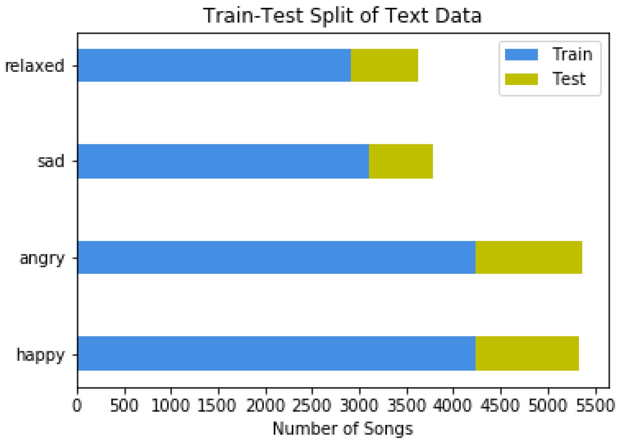
3.1. Lyrics Dataset Corpus, Features and Preprocessing
Proposed Words Embeddings
- Bag of WordsThe corpus preprocessing included the replacement of all the uppercase characters of the English alphabet with the corresponding lowercase characters, the removal of all punctuation and English stopwords (e.g., “the”,“is”,“at”,“which” …). Then, the preprocessing continues with the stemming procedure to reduce the derived words to their base stems, the tokenization of the input text in tokens and the rendering of IDs in the terms. After embedding the input data with the BoW method, our vocabulary size is . From the vocabulary, the 10,000 most common words are chosen to be used for the representation of the texts. Thus, each quatrain is represented by a vector of 10,000 in length, where each element corresponds with the number of occurrences of the corresponding vocabulary word in the quatrain. At the embedding layer layer of model the input vectors are compressed into dense vectors of length .
- TF-IDFThe preprocessing in the TF-IDF method is the same as in the BoW method. The vocabulary size is the same and the 10,000 words with the highest frequency terms are retained. This time, however, the words are represented by the resulting vectors according to the relation (8). Again, at the embedding layer, the input vectors are compressed into dense vectors of length 128.
- Word2VecBefore the Word2Vec method, a preprocessing takes place, converting all characters to lowercase and removing punctuation, numeric characters and stopwords. The processed input sequences are used to train the model. The model produces vectors of length , representing the sentences of each sequence. The value is the maximum number of words in the input sequences, each element represents one word in the input sequence, and the remaining elements are replaced by zeros.At the embedding layer its dimension is set to while this time the embedding initializer is also defined as the table, dimension x, which consists of the integrations of all of vocabulary words and converts each input word to the corresponding vector (embedding vector).
- GloVeThe GloVe method uses the same procedure as Word2Vec to preprocess the input sequences. For word embedding, GloVe provides default pretrained representations. It is essentially a 400,000-word vocabulary with pretrained representation vectors of length 100. From these vectors, the 400,000 × 100 co-occurrence matrix is constructed, which will then replace its untrained weights in the level of integration. Because the GloVe model uses finite vocabulary, it ignores words outside the vocabulary and it replaces their vectors with zeros.
- BERT EmbeddingsBERT’s tokenizer on the other side does not require any further preprocessing from our side. The mechanism (tokenizer) BERT uses is responsible for all preprocessing taking place in the input sentences, before training the model.Specifically, the tokenizer accepts at its input the texts for tokenization and creates a sequence of terms-words matching each input word in the corresponding term provided by its vocabulary, while maintaining occurrence order of words. For input words that are not recognized in the vocabulary, the tokenizer will try to break them down in vocabulary tokens to the maximum number of characters, in the worst case it will split a word into the characters that make it up. In the case of splitting a word the first token will appear in the sequence as it is, while the other tokens will appear augmented by the double symbol # at the beginning, so the model can identify which tokens are the results of splitting. For example, the word “playing” will be split into tokens “play” and “##ing”.
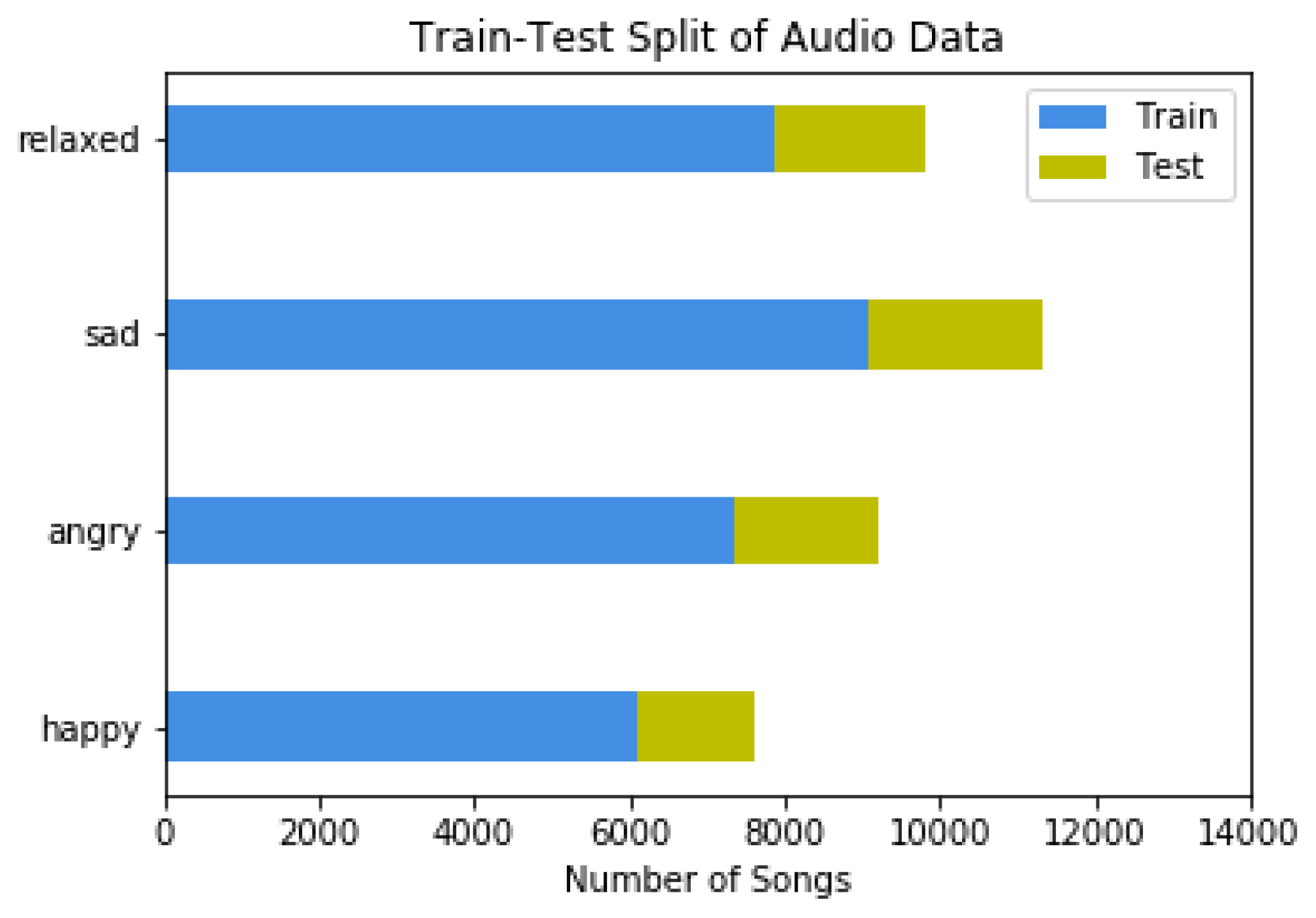
3.2. Audio Dataset Corpus, Features and Preprocessing
4. Methods
4.1. Lyric Analysis Subsystem
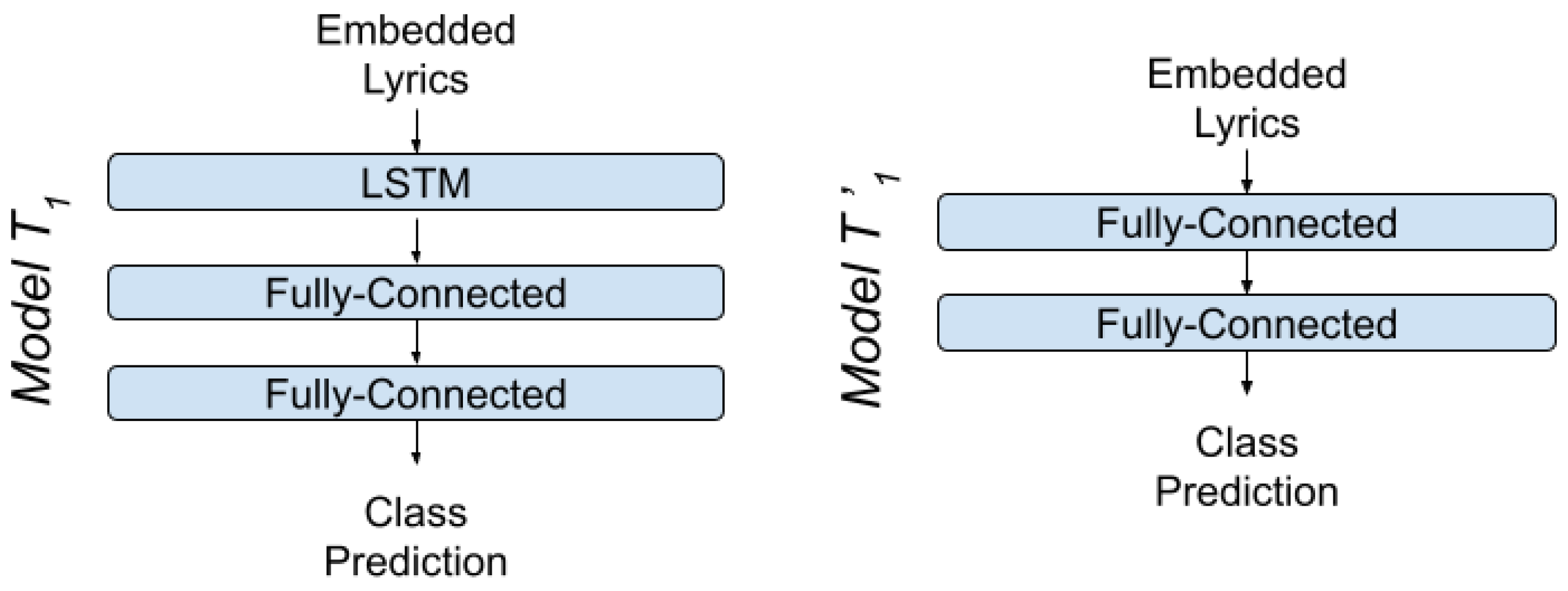
4.1.1. LSTM-MLP Models
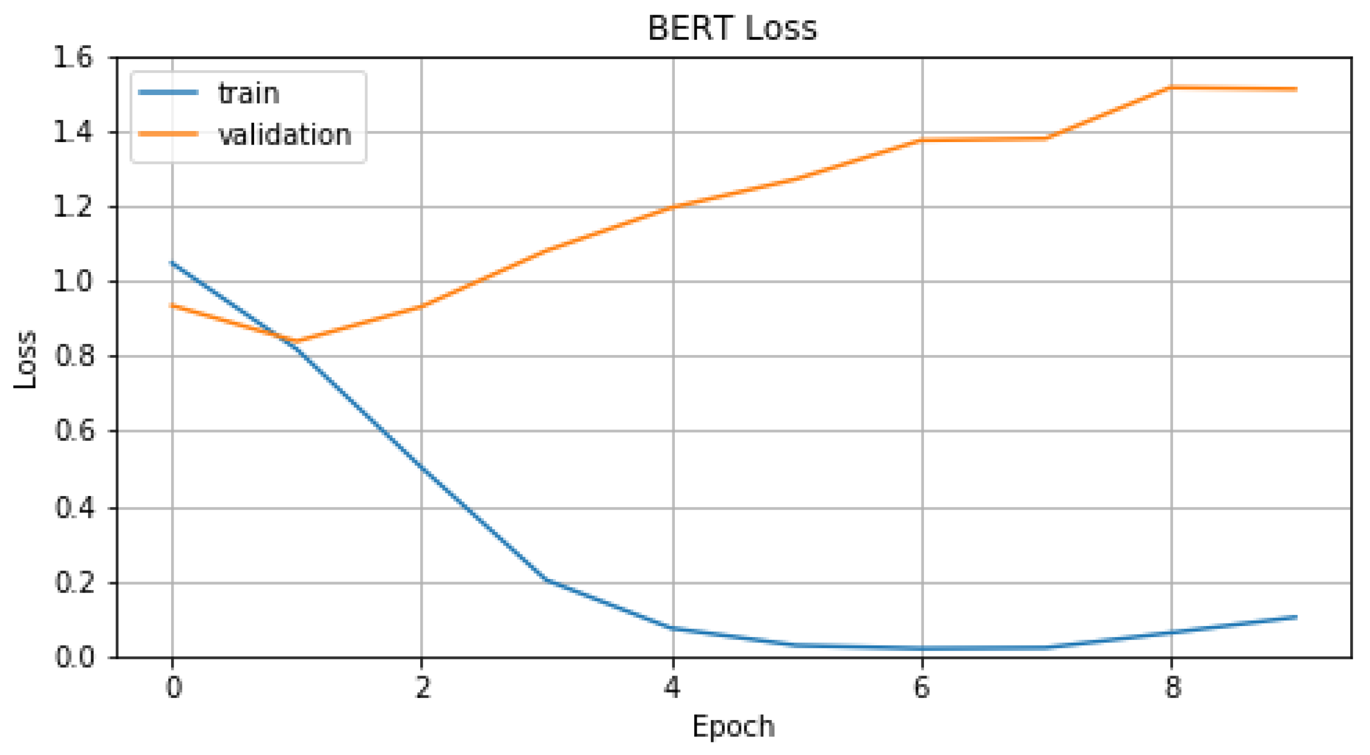
4.1.2. BERT Model
4.2. Audio Analysis Subsystem
4.3. Fuse Analysis System
5. Experimental Results
5.1. Lyric Analysis Subsystem
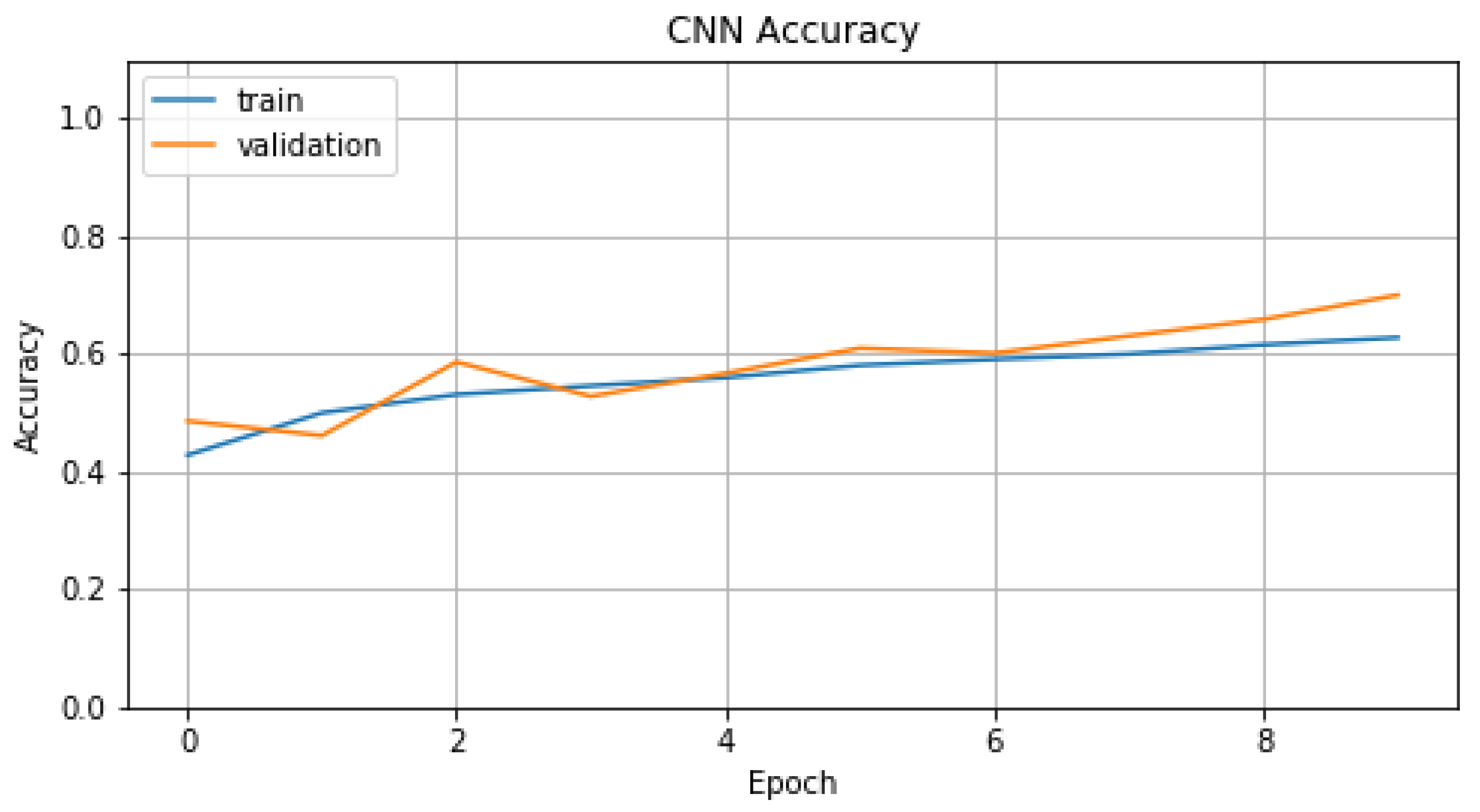
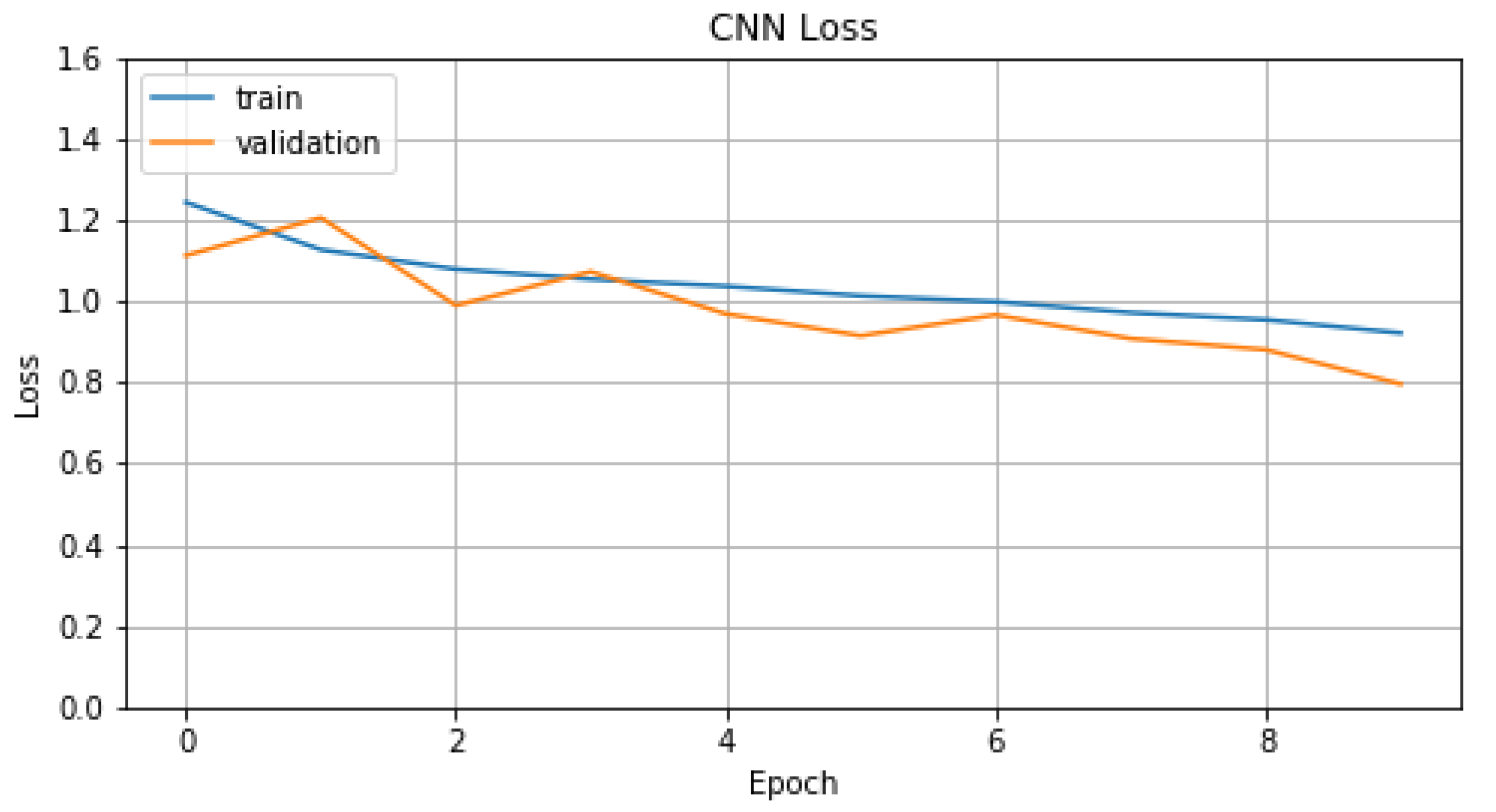
5.2. Audio Analysis Subsystem
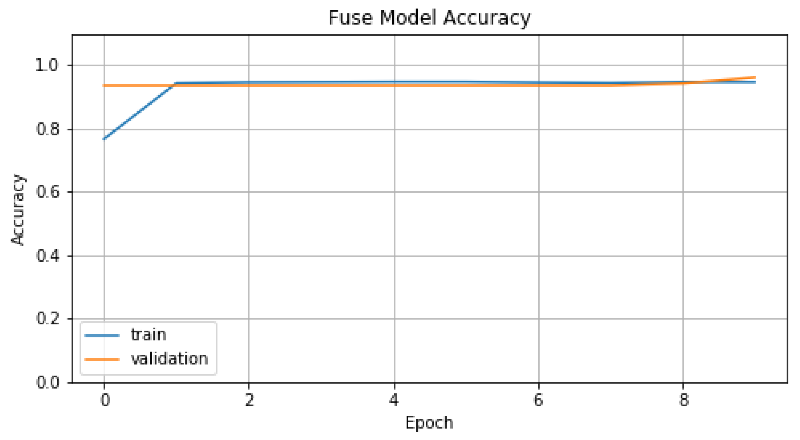
5.3. Fuse Analysis System
6. Conclusions and Future Work
Author Contributions
Funding
Institutional Review Board Statement
Informed Consent Statement
Data Availability Statement
Conflicts of Interest
References
- Hunter, P.; Schellenberg, E. Music and Emotion: Theory and Research; Oxford University Press: Oxford, UK, 2010; Volume 10, pp. 129–164. [Google Scholar] [CrossRef]
- Choi, K.; Fazekas, G.; Sandler, M.B.; Cho, K. Transfer Learning for Music Classification and Regression Tasks. arXiv 2017, arXiv:1703.09179. [Google Scholar]
- Schedl, M.; Zamani, H.; Chen, C.W.; Deldjoo, Y.; Elahi, M. Current challenges and visions in music recommender systems research. Int. J. Multimed. Inf. Retr. 2018, 7, 95–116. [Google Scholar] [CrossRef] [Green Version]
- Hennequin, R.; Khlif, A.; Voituret, F.; Moussallam, M. Spleeter: A fast and efficient music source separation tool with pre-trained models. J. Open Source Softw. 2020, 5, 2154. [Google Scholar] [CrossRef]
- Solanki, A.; Pandey, S. Music instrument recognition using deep convolutional neural networks. Int. J. Inf. Technol. 2019, 1–10. [Google Scholar] [CrossRef]
- Dong, H.W.; Hsiao, W.Y.; Yang, L.C.; Yang, Y.H. MuseGAN: Multi-Track Sequential Generative Adversarial Networks for Symbolic Music Generation and Accompaniment; AAAI: Menlo Park, CA, USA, 2018. [Google Scholar]
- Bruner, G. Music, Mood, and Marketing. J. Mark. 1990, 54, 94–104. [Google Scholar] [CrossRef]
- Zaanen, M.; Kanters, P. Automatic Mood Classification Using TF*IDF Based on Lyrics. In Proceedings of the ISMIR, Utrecht, The Netherlands, 9–13 August 2010; pp. 75–80. [Google Scholar]
- Tzanetakis, G. Marsyas Submissions to Mirex 2007. 2007. Available online: https://www.researchgate.net/profile/George-Tzanetakis/publication/228542053_MARSYAS_submissions_to_MIREX_2009/links/09e4150f71a5cdc52e000000/MARSYAS-submissions-to-MIREX-2009.pdf (accessed on 15 December 2021).
- Peeters, G. A Generic Training and Classification System for MIREX08 Classification Tasks: Audio Music Mood, Audio Genre, Audio Artist and Audio Tag. In Proceedings of the International Symposium on Music Information Retrieval, hiladelphia, PA, USA, 14–18 September 2008. [Google Scholar]
- Lidy, T.; Schindler, A. Parallel Convolutional Neural Networks for Music Genre and Mood Classification. 2016. Available online: http://www.ifs.tuwien.ac.at/~schindler/pubs/MIREX2016.pdf (accessed on 15 December 2021).
- Agrawal, Y.; Guru Ravi Shanker, R.; Alluri, V. Transformer-based approach towards music emotion recognition from lyrics. arXiv 2021, arXiv:2101.02051. [Google Scholar]
- Yang, Z.; Dai, Z.; Yang, Y.; Carbonell, J.; Salakhutdinov, R.; Le, Q.V. XLNet: Generalized Autoregressive Pretraining for Language Understanding. arXiv 2020, arXiv:1906.08237. [Google Scholar]
- Malheiro, R.; Panda, R.; Gomes, P.; Paiva, R.P. Bi-Modal Music Emotion Recognition: Novel Lyrical Features and Dataset. 2016. Available online: https://estudogeral.uc.pt/handle/10316/95162 (accessed on 15 December 2021).
- Hu, X.; Choi, K.; Downie, J. A framework for evaluating multimodal music mood classification. J. Assoc. Inf. Sci. Technol. 2016, 68. [Google Scholar] [CrossRef]
- Delbouys, R.; Hennequin, R.; Piccoli, F.; Royo-Letelier, J.; Moussallam, M. Music Mood Detection Based on Audio and Lyrics with Deep Neural Net. arXiv 2018, arXiv:1809.07276. [Google Scholar]
- Pyrovolakis, K.; Tzouveli, P.; Stamou, G. Mood detection analyzing lyrics and audio signal based on deep learning architectures. In Proceedings of the 2020 25th International Conference on Pattern Recognition (ICPR), Milan, Italy, 10–15 January 2021; pp. 9363–9370. [Google Scholar] [CrossRef]
- Erion Cano, M.M. MoodyLyrics: A Sentiment Annotated Lyrics Dataset. In Proceedings of the 2017 International Conference on Intelligent Systems, Metaheuristics & Swarm Intelligence, Hong Kong, China, 25–27 March 2017. [Google Scholar] [CrossRef] [Green Version]
- Susino, M.; Schubert, E. Cross-cultural anger communication in music: Towards a stereotype theory of emotion in music. Music. Sci. 2017, 21, 60–74. [Google Scholar] [CrossRef]
- Koelsch, S.; Fritz, T.; Cramon, D.Y.; Müller, K.; Friederici, A.D. Investigating emotion with music: An fMRI study. Hum. Brain Mapp. 2006, 27, 239–250. [Google Scholar] [CrossRef] [PubMed]
- Tao Li, M.O. Detecting Emotion in Music. 2003. Available online: https://jscholarship.library.jhu.edu/handle/1774.2/41 (accessed on 15 December 2021).
- Gabrielsson, A.; Lindström, E. The Influence of Musical Structure on Emotional Expression. 2001. Available online: https://psycnet.apa.org/record/2001-05534-004 (accessed on 15 December 2021).
- Music and Emotion. Available online: https://psycnet.apa.org/record/2012-14631-015 (accessed on 14 July 2020).
- Stevens, S.S.; Volkmann, J.; Newman, E.B. A Scale for the Measurement of the Psychological Magnitude Pitch. J. Acoust. Soc. Am. 1937, 8, 185–190. [Google Scholar] [CrossRef]
- Müller, M.; Kurth, F.; Clausen, M. Audio Matching via Chroma-Based Statistical Features. In Proceedings of the ISMIR, London, UK, 11–15 September 2005; pp. 288–295. [Google Scholar]
- Schoenberg, A.; Stein, L. Structural Functions of Harmony; Norton Library, W.W. Norton: New York, NY, USA, 1969. [Google Scholar]
- Plomp, R.; Pols, L.C.W.; van de Geer, J.P. Dimensional Analysis of Vowel Spectra. J. Acoust. Soc. Am. 1967, 41, 707–712. [Google Scholar] [CrossRef]
- Jiang, D.-N.; Lu, L.; Zhang, H.-J.; Tao, J.-H.; Cai, L.-H. Music type classification by spectral contrast feature. In Proceedings of the IEEE International Conference on Multimedia and Expo, Lausanne, Switzerland, 26–29 August 2002; Volume 1, pp. 113–116. [Google Scholar]
- Cohn, R. Introduction to Neo-Riemannian Theory: A Survey and a Historical Perspective. J. Music. Theory 1998, 42, 167–180. [Google Scholar] [CrossRef]
- Russell, J. A circumplex model of affect. J. Personal. Soc. Psychol. 1980, 39, 1161–1178. [Google Scholar] [CrossRef]
- Zhang, Y.; Jin, R.; Zhou, Z.H. Understanding bag-of-words model: A statistical framework. Int. J. Mach. Learn. Cybern. 2010, 1, 43–52. [Google Scholar] [CrossRef]
- Qaiser, S.; Ali, R. Text Mining: Use of TF-IDF to Examine the Relevance of Words to Documents. Int. J. Comput. Appl. 2018, 181. [Google Scholar] [CrossRef]
- Goldberg, Y.; Levy, O. word2vec Explained: Deriving Mikolov et al.’s Negative-Sampling Word-Embedding Method. arXiv 2014, arXiv:1402.3722. [Google Scholar]
- Pennington, J.; Socher, R.; Manning, C.D. GloVe: Global Vectors for Word Representation. In Proceedings of the Empirical Methods in Natural Language Processing (EMNLP), Doha, Qatar, 25–29 October 2014; pp. 1532–1543. [Google Scholar]
- Devlin, J.; Chang, M.W.; Lee, K.; Toutanova, K. BERT: Pre-training of Deep Bidirectional Transformers for Language Understanding. arXiv 2018, arXiv:1810.04805. [Google Scholar]
- Mikolov, T.; Chen, K.; Corrado, G.; Dean, J. Efficient Estimation of Word Representations in Vector Space. arXiv 2013, arXiv:1301.3781. [Google Scholar]
- Makarenkov, V.; Shapira, B.; Rokach, L. Language Models with Pre-Trained (GloVe) Word Embeddings. arXiv 2016, arXiv:1610.03759. [Google Scholar]
- Ryan, S.; Joseph, M.; Thomas, J. Characterization of the Affective Norms for English Words by discrete emotional categories. Behav. Res. Methods 2007, 39, 1020–1024. [Google Scholar] [CrossRef]
- Miller, G.A. WordNet: A Lexical Database for English. Commun. ACM 1995, 38, 39–41. [Google Scholar] [CrossRef]
- Valitutti, R. WordNet-Affect: An Affective Extension of WordNet. In Proceedings of the 4th International Conference on Language Resources and Evaluation, Lisbon, Portugal, 26–28 May 2004; pp. 1083–1086. [Google Scholar]
- Voulodimos, A.; Doulamis, N.; Doulamis, A.; Protopapadakis, E. Deep Learning for Computer Vision: A Brief Review. Comput. Intell. Neurosci. 2018, 2018, 7068349. [Google Scholar] [CrossRef]
- Guo, Y.; Liu, Y.; Oerlemans, A.; Lao, S.; Wu, S.; Lew, M.S. Deep learning for visual understanding: A review. Neurocomputing 2016, 187, 27–48. [Google Scholar] [CrossRef]
- Hochreiter, S.; Schmidhuber, J. Long Short-Term Memory. Neural Comput. 1997, 9, 1735–1780. [Google Scholar] [CrossRef] [PubMed]
- Vaswani, A.; Shazeer, N.; Parmar, N.; Uszkoreit, J.; Jones, L.; Gomez, A.N.; Kaiser, L.; Polosukhin, I. Attention Is All You Need. arXiv 2017, arXiv:1706.03762. [Google Scholar]
- Ioffe, S.; Szegedy, C. Batch Normalization: Accelerating Deep Network Training by Reducing Internal Covariate Shift. In Proceedings of the International Conference on Machine Learning, Lille, France, 6–11 July 2015. [Google Scholar]
- Abdillah, J.; Asror, I.; Wibowo, Y.F.A. Emotion Classification of Song Lyrics Using Bidirectional LSTM Method with GloVe Word Representation Weighting. J. RESTI 2020, 4, 723–729. [Google Scholar] [CrossRef]
- Çano, E. A Deep Learning Architecture for Sentiment Analysis. In Proceedings of the International Conference on Geoinformatics and Data Analysis, Prague, Czech Republic, 20–22 April 2018. [Google Scholar] [CrossRef] [Green Version]
- Siriket, K.; Sa-Ing, V.; Khonthapagdee, S. Mood classification from Song Lyric using Machine Learning. In Proceedings of the 2021 9th International Electrical Engineering Congress (iEECON), Pattaya, Thailand, 10–12 March 2021; pp. 476–478. [Google Scholar]
- Çano, E.; Morisio, M. A Data-driven Neural Network Architecture for Sentiment Analysis. Data Technol. Appl. 2019, 53. [Google Scholar] [CrossRef]
- Deep Mood Detection. Available online: https://github.com/konpyro/DeepMoodDetection (accessed on 15 December 2021).


| Structural Feature | Definition | Associated Emotion |
|---|---|---|
| Tempo | The speed or pace of a musical piece | Fast tempo: happiness, excitement, anger. Slow tempo: sadness, serenity. |
| Mode | The type of scale | Major tonality: happiness, joy. Minor tonality: sadness. |
| Loudness | The physical strength and amplitude of a sound | Intensity, power, or anger |
| Melody | The linear succession of musical tones that the listener perceives as a single entity | Complementing harmonies: happiness, relaxation, serenity. Clashing harmonies: excitement, anger, unpleasantness. |
| Rhythm | The regularly recurring pattern or beat of a song | Smooth/consistent rhythm: happiness, peace. Rough/irregular rhythm: amusement, uneasiness. Varied rhythm: joy. |
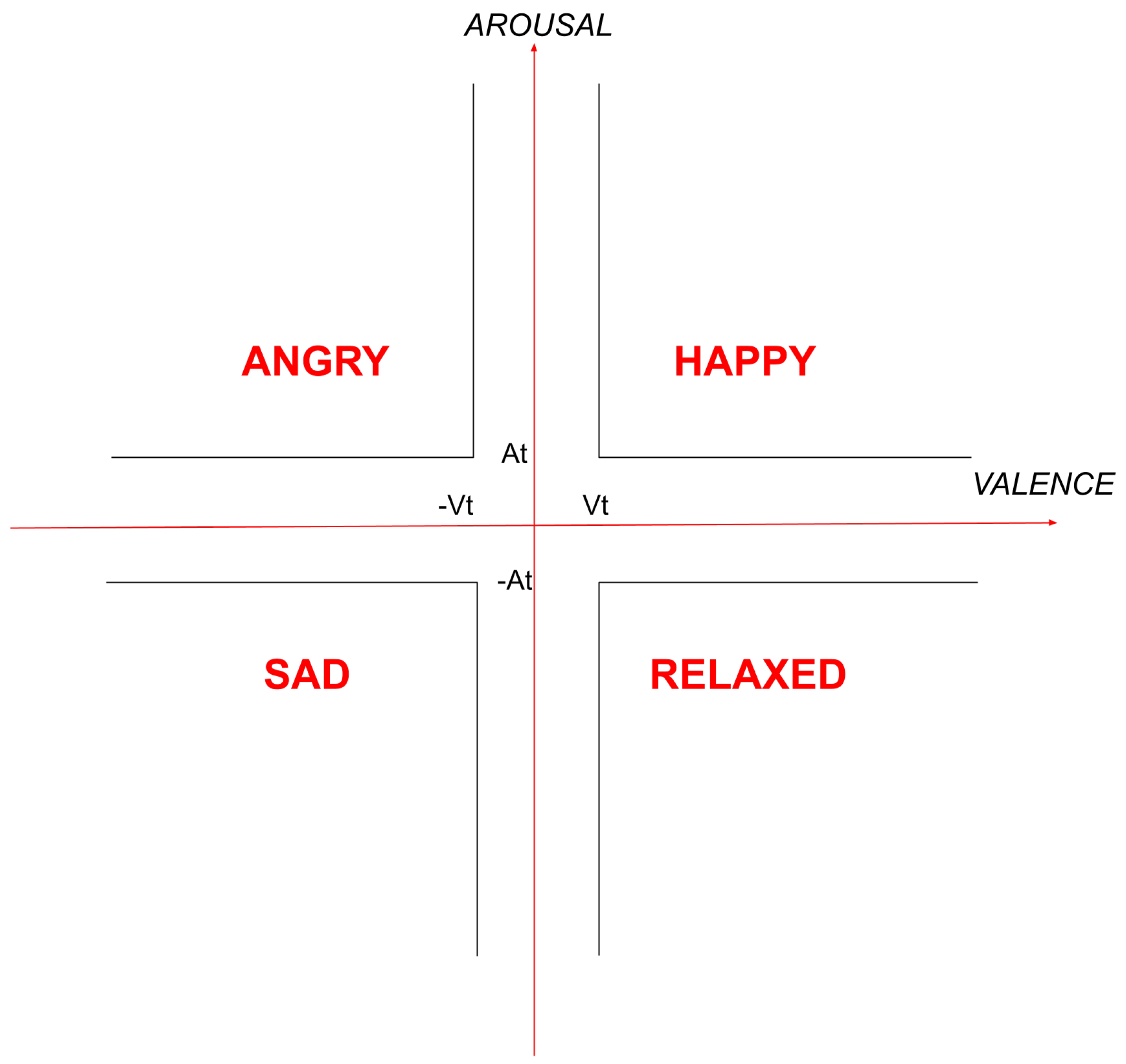
| Valence (V) and Arousal (A) Values | Mood |
|---|---|
| and | Happy |
| and | Angry |
| and | Sad |
| and | Relaxed |
| Model | Embedding Method | Loss | Accuracy (%) |
|---|---|---|---|
| BoW | 1.287 | 65.49 | |
| TF-IDF | 1.381 | 67.98 | |
| Word2Vec | 1.262 | 41.66 | |
| GloVe | 1.064 | 53.33 | |
| Bert | 1.353 | 69.11 |
| Feature Combination | Accuracy (%) |
|---|---|
| Mel | 64.97 |
| Mel, Log-Mel | 68.38 |
| Mel, Chroma, Tonnetz, Spectral Contrast | 60.86 |
| Log-Mel, Chroma, Tonnetz, Spectral Contrast | 58.96 |
| MFCC, Chroma, Tonnetz, Spectral Contrast | 65.36 |
| Mel, Log-Mel, MFCC, Chroma, Tonnetz | 69.77 |
| Mel, Log-Mel, MFCC, Chroma, Tonnetz, Spectral Contrast | 70.34 |
| Model | Loss | Accuracy (%) |
|---|---|---|
| 1.381 | 67.98 | |
| 1.353 | 69.11 | |
| 0.743 | 70.51 |
| Model | Loss | Accuracy (%) | Computational Time |
|---|---|---|---|
| 1.381 | 67.98 | 0 m 25.391 s | |
| 1.353 | 69.11 | 18 m 12.444 s | |
| 0.743 | 70.51 | 80 m 13.064 s | |
| 0.156 | 94.58 | 3 m 38.551 s |
Publisher’s Note: MDPI stays neutral with regard to jurisdictional claims in published maps and institutional affiliations. |
© 2022 by the authors. Licensee MDPI, Basel, Switzerland. This article is an open access article distributed under the terms and conditions of the Creative Commons Attribution (CC BY) license (https://creativecommons.org/licenses/by/4.0/).
Share and Cite
Pyrovolakis, K.; Tzouveli, P.; Stamou, G. Multi-Modal Song Mood Detection with Deep Learning. Sensors 2022, 22, 1065. https://doi.org/10.3390/s22031065
Pyrovolakis K, Tzouveli P, Stamou G. Multi-Modal Song Mood Detection with Deep Learning. Sensors. 2022; 22(3):1065. https://doi.org/10.3390/s22031065
Chicago/Turabian StylePyrovolakis, Konstantinos, Paraskevi Tzouveli, and Giorgos Stamou. 2022. "Multi-Modal Song Mood Detection with Deep Learning" Sensors 22, no. 3: 1065. https://doi.org/10.3390/s22031065
APA StylePyrovolakis, K., Tzouveli, P., & Stamou, G. (2022). Multi-Modal Song Mood Detection with Deep Learning. Sensors, 22(3), 1065. https://doi.org/10.3390/s22031065