
Efficient Spatiotemporal Attention Network for Remote Heart Rate Variability Analysis


Abstract
:1. Introduction
2. Related Work
3. Materials and Methods
3.1. Data Pre-Processing
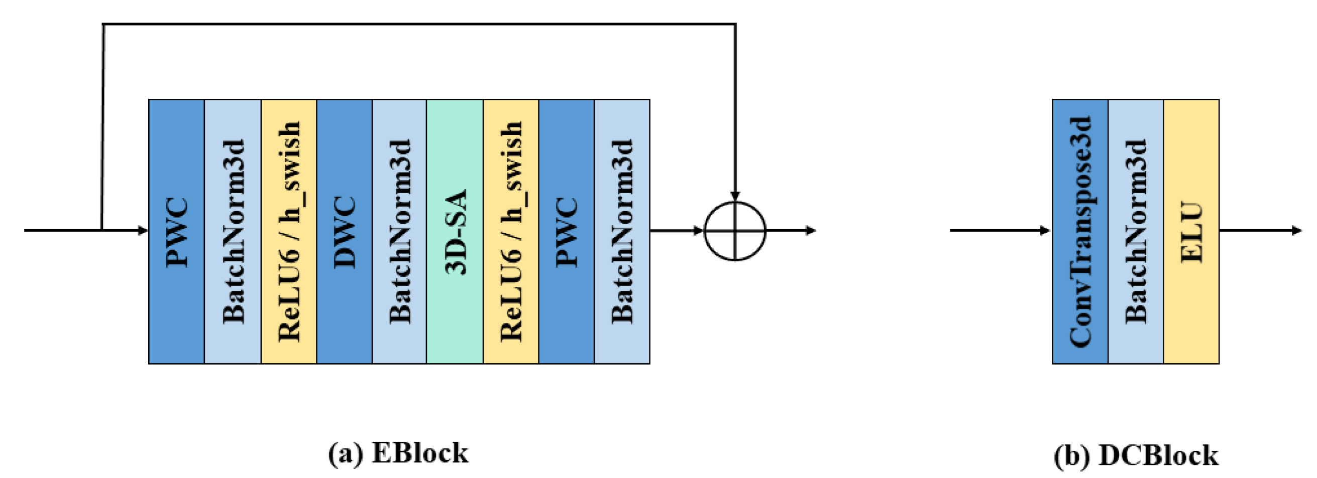
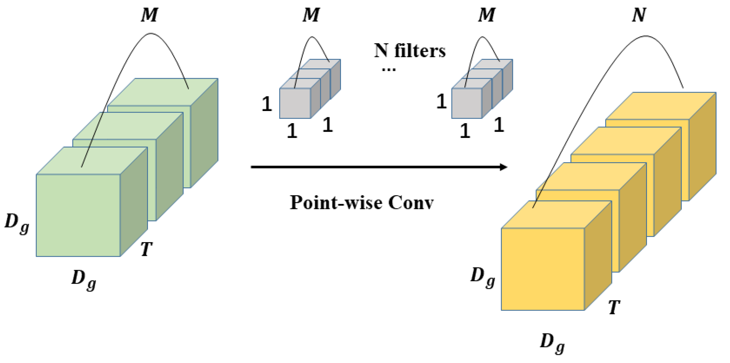
3.2. 3D Depth-Wise Separable Convolution
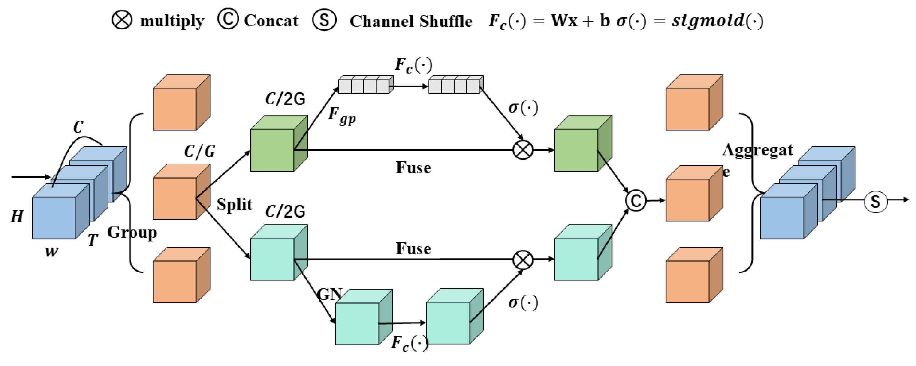
3.3. 3D Shuffle Attention Block
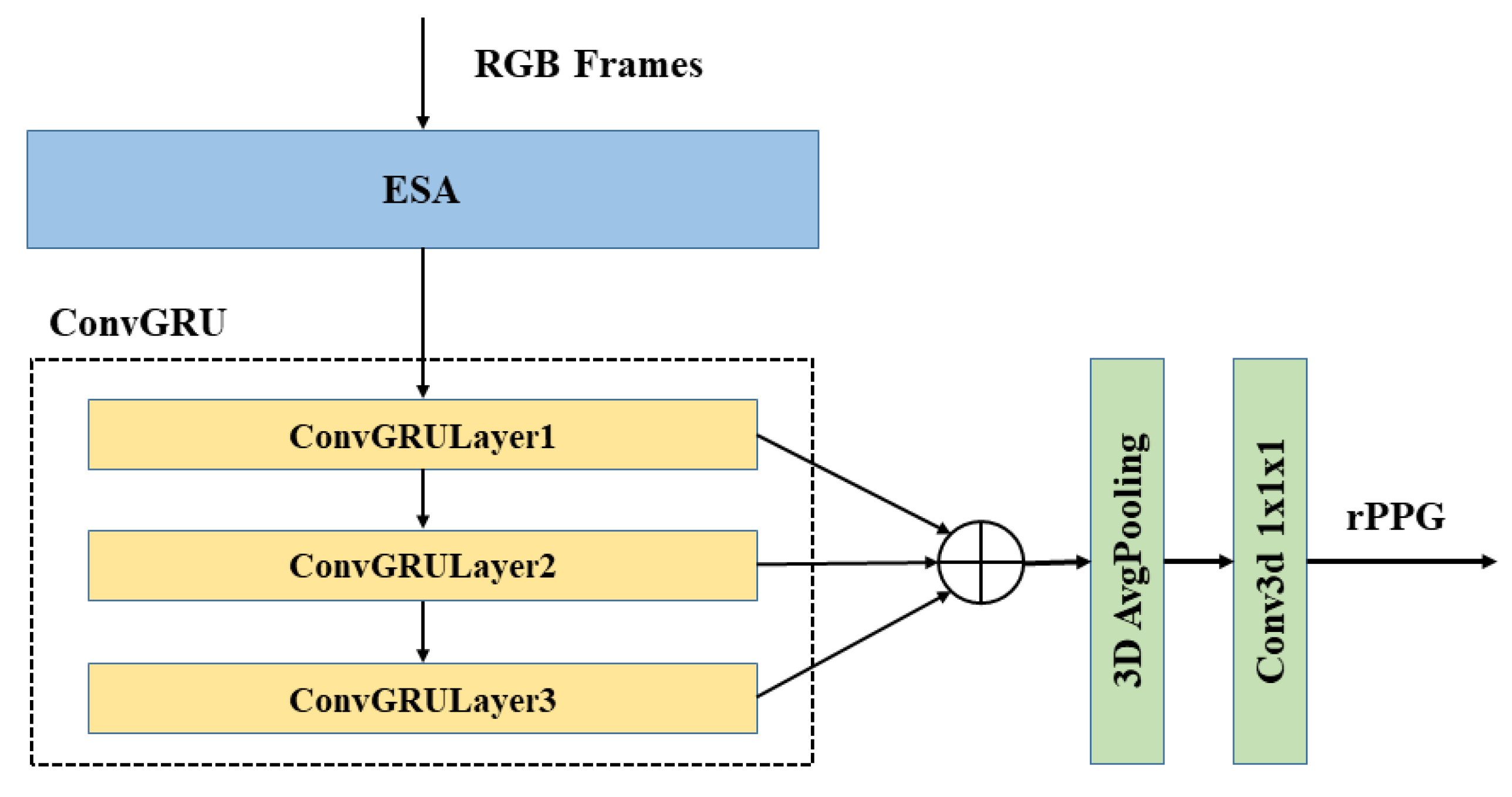
3.4. Recurrent Neural Network ConvGRU
3.5. ESA-rPPGNet
3.6. Loss Function
3.7. Signal Post-Processing
4. Experiments and Result
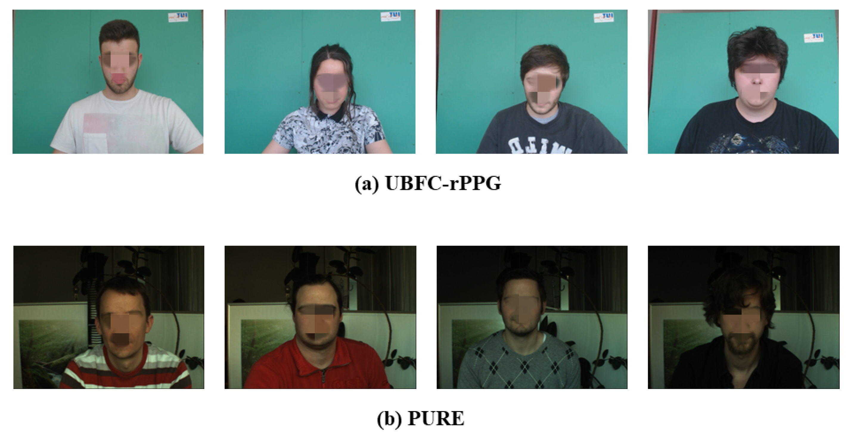
4.1. Datasets
4.2. Experimental Setup
4.3. Evaluation Metrics
4.4. Experimental Results
5. Conclusions and Discussion
Author Contributions
Funding
Conflicts of Interest
References
- Dekker, J.M.; Schouten, E.G.; Klootwijk, P.; Pool, J.; Swenne, C.A.; Kromhout, D. Heart rate variability from short electrocardiographic recordings predicts mortality from all causes in middle-aged and elderly men: The Zutphen Study. Am. J. Epidemiol. 1997, 145, 899–908. [Google Scholar] [CrossRef] [PubMed] [Green Version]
- Kranjec, J.; Beguš, S.; Geršak, G.; Drnovšek, J. Non-contact heart rate and heart rate variability measurements: A review. Biomed. Signal Process. Control 2014, 13, 102–112. [Google Scholar] [CrossRef]
- Hassan, M.A.; Malik, A.S.; Fofi, D.; Saad, N.; Karasfi, B.; Ali, Y.S.; Meriaudeau, F. Heart rate estimation using facial video: A review. Biomed. Signal Process. Control 2017, 38, 346–360. [Google Scholar] [CrossRef]
- Al-Naji, A.; Gibson, K.; Lee, S.H.; Chahl, J. Monitoring of cardiorespiratory signal: Principles of remote measurements and review of methods. IEEE Access 2017, 5, 15776–15790. [Google Scholar] [CrossRef]
- Balakrishnan, G.; Durand, F.; Guttag, J. Detecting pulse from head motions in video. In Proceedings of the IEEE Conference on Computer Vision and Pattern Recognition, Portland, OR, USA, 23–28 June 2013; pp. 3430–3437. [Google Scholar]
- Li, X.; Chen, J.; Zhao, G.; Pietikainen, M. Remote heart rate measurement from face videos under realistic situations. In Proceedings of the IEEE Conference on Computer Vision and Pattern Recognition, Columbus, OH, USA, 23–28 June 2014; pp. 4264–4271. [Google Scholar]
- Poh, M.Z.; McDuff, D.J.; Picard, R.W. Non-contact, automated cardiac pulse measurements using video imaging and blind source separation. Opt. Express 2010, 18, 10762–10774. [Google Scholar] [CrossRef]
- Lewandowska, M.; Rumiński, J.; Kocejko, T.; Nowak, J. Measuring pulse rate with a webcam—A non-contact method for evaluating cardiac activity. In Proceedings of the 2011 Federated Conference on Computer Science and Information Systems (FedCSIS), Szczecin, Poland, 18–21 September 2011; IEEE: Piscataway, NJ, USA, 2011; pp. 405–410. [Google Scholar]
- De Haan, G.; Jeanne, V. Robust pulse rate from chrominance-based rPPG. IEEE Trans. Biomed. Eng. 2013, 60, 2878–2886. [Google Scholar] [CrossRef]
- Wang, W.; den Brinker, A.C.; Stuijk, S.; De Haan, G. Algorithmic principles of remote PPG. IEEE Trans. Biomed. Eng. 2016, 64, 1479–1491. [Google Scholar] [CrossRef] [Green Version]
- Gudi, A.; Bittner, M.; van Gemert, J. Real-Time Webcam Heart-Rate and Variability Estimation with Clean Ground Truth for Evaluation. Appl. Sci. 2020, 10, 8630. [Google Scholar] [CrossRef]
- Chen, W.; McDuff, D. Deepphys: Video-based physiological measurement using convolutional attention networks. In Proceedings of the European Conference on Computer Vision (ECCV), Munich, Germany, 8–14 September 2018; pp. 349–365. [Google Scholar]
- Špetlík, R.; Franc, V.; Matas, J. Visual heart rate estimation with convolutional neural network. In Proceedings of the British Machine Vision Conference, Newcastle, UK, 3–6 September 2018; pp. 3–6. [Google Scholar]
- Niu, X.; Han, H.; Shan, S.; Chen, X. Synrhythm: Learning a deep heart rate estimator from general to specific. In Proceedings of the 2018 24th International Conference on Pattern Recognition (ICPR), Beijing, China, 20–24 August 2018; IEEE: Piscataway, NJ, USA, 2018; pp. 3580–3585. [Google Scholar]
- Lee, E.; Chen, E.; Lee, C.Y. Meta-rppg: Remote heart rate estimation using a transductive meta-learner. In Proceedings of the European Conference on Computer Vision, Glasgow, UK, 23–28 August 2020; Springer: Berlin/Heidelberg, Germany, 2020; pp. 392–409. [Google Scholar]
- Rodríguez, A.M.; Ramos-Castro, J. Video pulse rate variability analysis in stationary and motion conditions. Biomed. Eng. Online 2018, 17, 11. [Google Scholar] [CrossRef] [Green Version]
- Finžgar, M.; Podržaj, P. Feasibility of assessing ultra-short-term pulse rate variability from video recordings. PeerJ 2020, 8, e8342. [Google Scholar] [CrossRef] [Green Version]
- Stricker, R.; Müller, S.; Gross, H.M. Non-contact video-based pulse rate measurement on a mobile service robot. In Proceedings of the 23rd IEEE International Symposium on Robot and Human Interactive Communication, Edinburgh, UK, 25–29 August 2014; IEEE: Piscataway, NJ, USA, 2014; pp. 1056–1062. [Google Scholar]
- Li, P.; Benezeth, Y.; Nakamura, K.; Gomez, R.; Li, C.; Yang, F. An improvement for video-based heart rate variability measurement. In Proceedings of the the 2019 IEEE 4th International Conference on Signal and Image Processing (ICSIP), Wuxi, China, 19–21 July 2019; IEEE: Piscataway, NJ, USA, 2019; pp. 435–439. [Google Scholar]
- Bobbia, S.; Macwan, R.; Benezeth, Y.; Mansouri, A.; Dubois, J. Unsupervised skin tissue segmentation for remote photoplethysmography. Pattern Recognit. Lett. 2019, 124, 82–90. [Google Scholar] [CrossRef]
- Gudi, A.; Bittner, M.; Lochmans, R.; van Gemert, J. Efficient real-time camera based estimation of heart rate and its variability. In Proceedings of the IEEE/CVF International Conference on Computer Vision Workshops, Seoul, Korea, 27–28 October 2019. [Google Scholar]
- Song, R.; Chen, H.; Cheng, J.; Li, C.; Liu, Y.; Chen, X. PulseGAN: Learning to generate realistic pulse waveforms in remote photoplethysmography. IEEE J. Biomed. Health Informatics 2021, 25, 1373–1384. [Google Scholar] [CrossRef] [PubMed]
- Niu, X.; Yu, Z.; Han, H.; Li, X.; Shan, S.; Zhao, G. Video-based remote physiological measurement via cross-verified feature disentangling. In Proceedings of the European Conference on Computer Vision, Glasgow, UK, 23–28 August 2020; Springer: Berlin/Heidelberg, Germany, 2020; pp. 295–310. [Google Scholar]
- Ji, S.; Xu, W.; Yang, M.; Yu, K. 3D convolutional neural networks for human action recognition. IEEE Trans. Pattern Anal. Mach. Intell. 2012, 35, 221–231. [Google Scholar] [CrossRef] [Green Version]
- Yu, Z.; Li, X.; Zhao, G. Remote photoplethysmograph signal measurement from facial videos using spatio-temporal networks. arXiv 2019, arXiv:1905.02419. [Google Scholar]
- Zhang, K.; Zhang, Z.; Li, Z.; Qiao, Y. Joint face detection and alignment using multitask cascaded convolutional networks. IEEE Signal Process. Lett. 2016, 23, 1499–1503. [Google Scholar] [CrossRef] [Green Version]
- Hu, J.; Shen, L.; Sun, G. Squeeze-and-excitation networks. In Proceedings of the IEEE Conference on Computer Vision and Pattern Recognition, Salt Lake City, UT, USA, 18–23 June 2018; pp. 7132–7141. [Google Scholar]
- Woo, S.; Park, J.; Lee, J.Y.; Kweon, I.S. Cbam: Convolutional block attention module. In Proceedings of the European Conference on Computer Vision (ECCV), Munich, Germany, 8–14 September 2018; pp. 3–19. [Google Scholar]
- Zhang, Q.L.; Yang, Y.B. Sa-net: Shuffle attention for deep convolutional neural networks. In Proceedings of the ICASSP 2021–2021 IEEE International Conference on Acoustics, Speech and Signal Processing (ICASSP), Toronto, ON, Canada, 6–11 June 2021; IEEE: Piscataway, NJ, USA, 2021; pp. 2235–2239. [Google Scholar]
- Ma, N.; Zhang, X.; Zheng, H.T.; Sun, J. Shufflenet v2: Practical guidelines for efficient cnn architecture design. In Proceedings of the European Conference on Computer Vision (ECCV), Munich, Germany, 8–14 September 2018; pp. 116–131. [Google Scholar]
- Wu, Y.; He, K. Group normalization. In Proceedings of the European Conference on Computer Vision (ECCV), Munich, Germany, 8–14 September 2018; pp. 3–19. [Google Scholar]
- Chung, J.; Gulcehre, C.; Cho, K.; Bengio, Y. Empirical evaluation of gated recurrent neural networks on sequence modeling. arXiv 2014, arXiv:1412.3555. [Google Scholar]
- Xingjian, S.; Chen, Z.; Wang, H.; Yeung, D.Y.; Wong, W.K.; Woo, W.c. Convolutional LSTM network: A machine learning approach for precipitation nowcasting. In Advances in Neural Information Processing Systems; MIT Press: Cambridge, MA, USA, 2015; pp. 802–810. [Google Scholar]
- Ballas, N.; Yao, L.; Pal, C.; Courville, A. Delving deeper into convolutional networks for learning video representations. arXiv 2015, arXiv:1511.06432. [Google Scholar]
- Howard, A.; Sandler, M.; Chu, G.; Chen, L.C.; Chen, B.; Tan, M.; Wang, W.; Zhu, Y.; Pang, R.; Vasudevan, V.; et al. Searching for mobilenetv3. In Proceedings of the IEEE/CVF International Conference on Computer Vision, Seoul, Korea, 27 October–2 November 2019; pp. 1314–1324. [Google Scholar]
- Lea, C.; Flynn, M.D.; Vidal, R.; Reiter, A.; Hager, G.D. Temporal convolutional networks for action segmentation and detection. In Proceedings of the IEEE Conference on Computer Vision and Pattern Recognition, Honolulu, HI, USA, 21–26 July 2017; pp. 156–165. [Google Scholar]
- Howard, A.; Zhmoginov, A.; Chen, L.C.; Sandler, M.; Zhu, M. Inverted residuals and linear bottlenecks: Mobile networks for classification, detection and segmentation. In Proceedings of the IEEE Conference on Computer Vision and Pattern Recognition, Salt Lake City, UT, USA, 18–23 June 2018. [Google Scholar]
- Ramachandran, P.; Zoph, B.; Le, Q.V. Searching for activation functions. arXiv 2017, arXiv:1710.05941. [Google Scholar]
- Kwon, O.; Jeong, J.; Kim, H.B.; Kwon, I.H.; Park, S.Y.; Kim, J.E.; Choi, Y. Electrocardiogram sampling frequency range acceptable for heart rate variability analysis. Healthc. Inform. Res. 2018, 24, 198–206. [Google Scholar] [CrossRef]
- Poh, M.Z.; McDuff, D.J.; Picard, R.W. Advancements in noncontact, multiparameter physiological measurements using a webcam. IEEE Trans. Biomed. Eng. 2010, 58, 7–11. [Google Scholar] [CrossRef] [Green Version]
- Verkruysse, W.; Svaasand, L.O.; Nelson, J.S. Remote plethysmographic imaging using ambient light. Opt. Express 2008, 16, 21434–21445. [Google Scholar] [CrossRef] [PubMed] [Green Version]


| Input | Operator | Exp Size | Opt Size | Stride | SA | NL |
|---|---|---|---|---|---|---|
| Conv3d, 3 × 3 × 3 | - | 16 | 1 × 2 × 2 | - | - | |
| EBlock, 3 × 3 × 3 | 16 | 16 | 1 × 2 × 2 | 1 | 0 | |
| EBlock, 3 × 3 × 3 | 72 | 24 | 1 × 2 × 2 | 0 | 0 | |
| EBlock, 3 × 3 × 3 | 88 | 24 | 1 × 1 × 1 | 0 | 0 | |
| EBlock, 5 × 5 × 5 | 96 | 40 | 2 × 2 × 2 | 1 | 1 | |
| EBlock, 5 × 5 × 5 | 240 | 40 | 1 × 1 × 1 | 1 | 1 | |
| EBlock, 5 × 5 × 5 | 240 | 40 | 1 × 1 × 1 | 1 | 1 | |
| EBlock, 5 × 5 × 5 | 120 | 48 | 1 × 1 × 1 | 1 | 1 | |
| EBlock, 5 × 5 × 5 | 144 | 48 | 1 × 1 × 1 | 1 | 1 | |
| EBlock, 5 × 5 × 5 | 288 | 96 | 2 × 2 × 2 | 1 | 1 | |
| EBlock, 5 × 5 × 5 | 576 | 96 | 1 × 1 × 1 | 1 | 1 | |
| EBlock, 5 × 5 × 5 | 576 | 96 | 1 × 1 × 1 | 1 | 1 | |
| Conv3d, 1 × 1 × 1 | - | 576 | 1 × 1 × 1 | - | - | |
| DCBlock, 4 × 1 × 1 | - | 288 | 2 × 1 × 1 | - | - | |
| DCBlock, 4 × 1 × 1 | - | 144 | 2 × 1 × 1 | - | - | |
| ConvGRU | - | 64 | - | - | - | |
| GAP | - | 64 | - | - | - | |
| Conv3d, 1 × 1 × 1 | - | 1 | 1 × 1 × 1 | - | - |
| Method | |||
|---|---|---|---|
| CHROM [9] | 16.54 | 40.90 | 93 |
| SSF [19] | - | 25 | 47 |
| FaceRPPG [21] | - | 19 | 16 |
| PulseGAN [22] | 7.52 | 18.36 | - |
| PhysNet [25] | 8.23 | 15.12 | 32.58 |
| Ours | 5.14 | 13.76 | 14.17 |
| Method | LF (u.n) | HF (u.n) | LF/HF | |||
|---|---|---|---|---|---|---|
| RMSE | R | RMSE | R | RMSE | R | |
| POS [10] | 0.169 | 0.479 | 0.169 | 0.479 | 0.399 | 0.518 |
| CHROM [9] | 0.240 | 0.159 | 0.240 | 0.159 | 0.645 | 0.226 |
| Green [41] | 0.186 | 0.280 | 0.186 | 0.280 | 0.365 | 0.492 |
| FaceRPPG [21] | 0.2 | - | 0.2 | - | 1.0 | - |
| CVD [23] | 0.065 | 0.740 | 0.065 | 0.740 | 0.168 | 0.812 |
| PhysNet [25] | 0.0984 | 0.8024 | 0.0984 | 0.8024 | 0.9734 | 0.7991 |
| Ours | 0.0546 | 0.9018 | 0.0546 | 0.9018 | 0.2191 | 0.9424 |
| Method | |||
|---|---|---|---|
| CHROM [9] | 49.63 | 89.30 | - |
| FaceRPPG [21] | - | 18 | 15 |
| PulseGAN [22] | 28.92 | 49.39 | - |
| PhysNet [25] | 12.34 | 14.22 | 34.16 |
| Ours | 8.92 | 11.75 | 26.12 |
| Method | LF (u.n) | HF (u.n) | LF/HF | |||
|---|---|---|---|---|---|---|
| RMSE | R | RMSE | R | RMSE | R | |
| FaceRPPG [21] | 0.1 | - | 0.1 | - | 1.3 | - |
| PhysNet [25] | 0.1115 | 0.8413 | 0.1115 | 0.8413 | 1.0710 | 0.8891 |
| Ours | 0.0824 | 0.9284 | 0.0824 | 0.9284 | 1.0441 | 0.9699 |
| Method | FLOPs (G) | Params (M) |
|---|---|---|
| PhysNet | 115.16 | 0.77 |
| Ours | 4.69 | 1.62 |
Publisher’s Note: MDPI stays neutral with regard to jurisdictional claims in published maps and institutional affiliations. |
© 2022 by the authors. Licensee MDPI, Basel, Switzerland. This article is an open access article distributed under the terms and conditions of the Creative Commons Attribution (CC BY) license (https://creativecommons.org/licenses/by/4.0/).
Share and Cite
Kuang, H.; Lv, F.; Ma, X.; Liu, X. Efficient Spatiotemporal Attention Network for Remote Heart Rate Variability Analysis. Sensors 2022, 22, 1010. https://doi.org/10.3390/s22031010
Kuang H, Lv F, Ma X, Liu X. Efficient Spatiotemporal Attention Network for Remote Heart Rate Variability Analysis. Sensors. 2022; 22(3):1010. https://doi.org/10.3390/s22031010
Chicago/Turabian StyleKuang, Hailan, Fanbing Lv, Xiaolin Ma, and Xinhua Liu. 2022. "Efficient Spatiotemporal Attention Network for Remote Heart Rate Variability Analysis" Sensors 22, no. 3: 1010. https://doi.org/10.3390/s22031010
APA StyleKuang, H., Lv, F., Ma, X., & Liu, X. (2022). Efficient Spatiotemporal Attention Network for Remote Heart Rate Variability Analysis. Sensors, 22(3), 1010. https://doi.org/10.3390/s22031010