

Estimation of Vehicle Longitudinal Velocity with Artificial Neural Network

 , ,
, ,  ,
,  ,
,  and
and 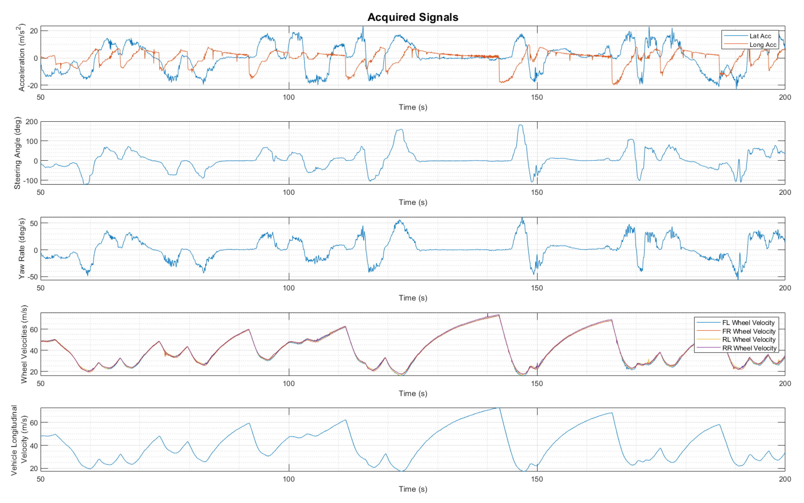
Abstract
1. Introduction
2. Equipped Sensors and Acquired Channels
2.1. Equipped Sensors
2.2. Acquired Channels
- steering angle [deg];
- lateral acceleration [m/s2];
- longitudinal acceleration [m/s2];
- yaw rate [deg/s];
- wheels speed [m/s];
- vehicle longitudinal velocity [m/s].
3. A Feed-Forward Neural Network-Based Longitudinal Velocity Estimation System
3.1. Input Data
- steering angle [deg];
- lateral acceleration [g];
- longitudinal acceleration [g];
- yaw rate [deg/s];
- wheels speed [km/h].
- vehicle longitudinal velocity [km/h].
3.2. Data Scaling
3.3. Preliminary Neural Network Design
3.4. Rprop
3.5. Analyzed Approaches
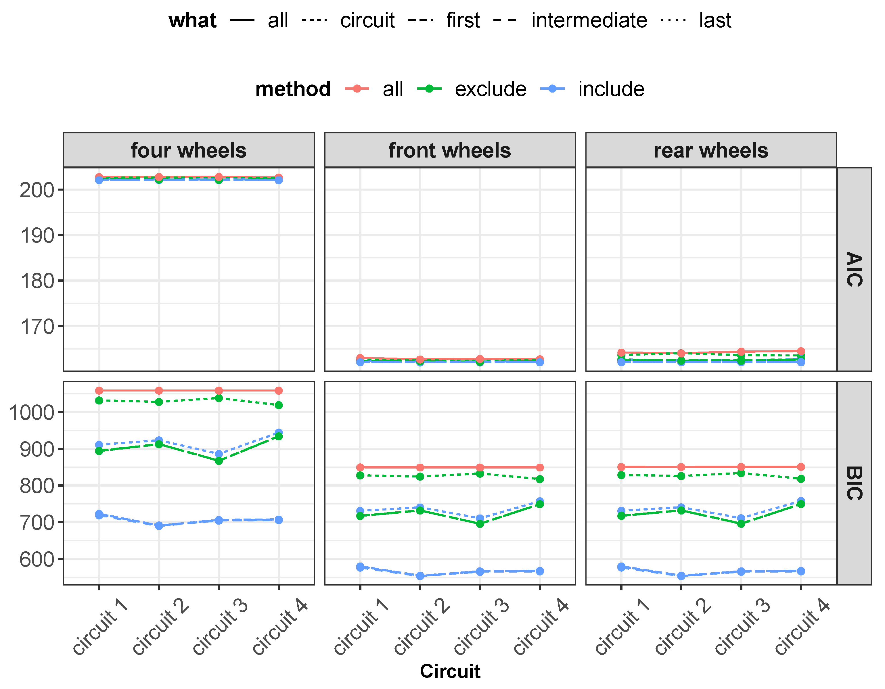
- All: Data from all laps and circuits are used to train and test the neural network. The system randomly selects the data to use for the training set while the remaining ones are used in the test set;
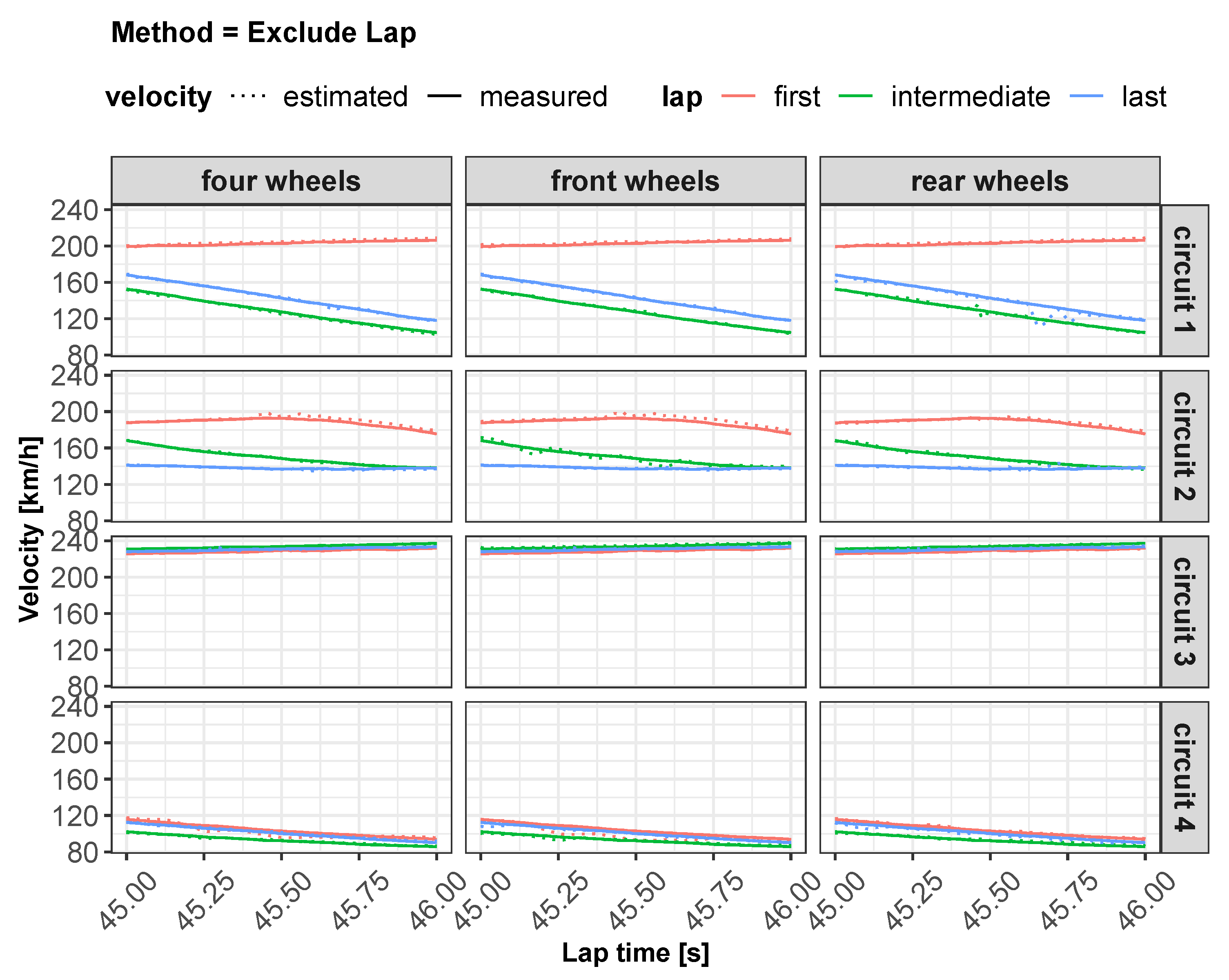
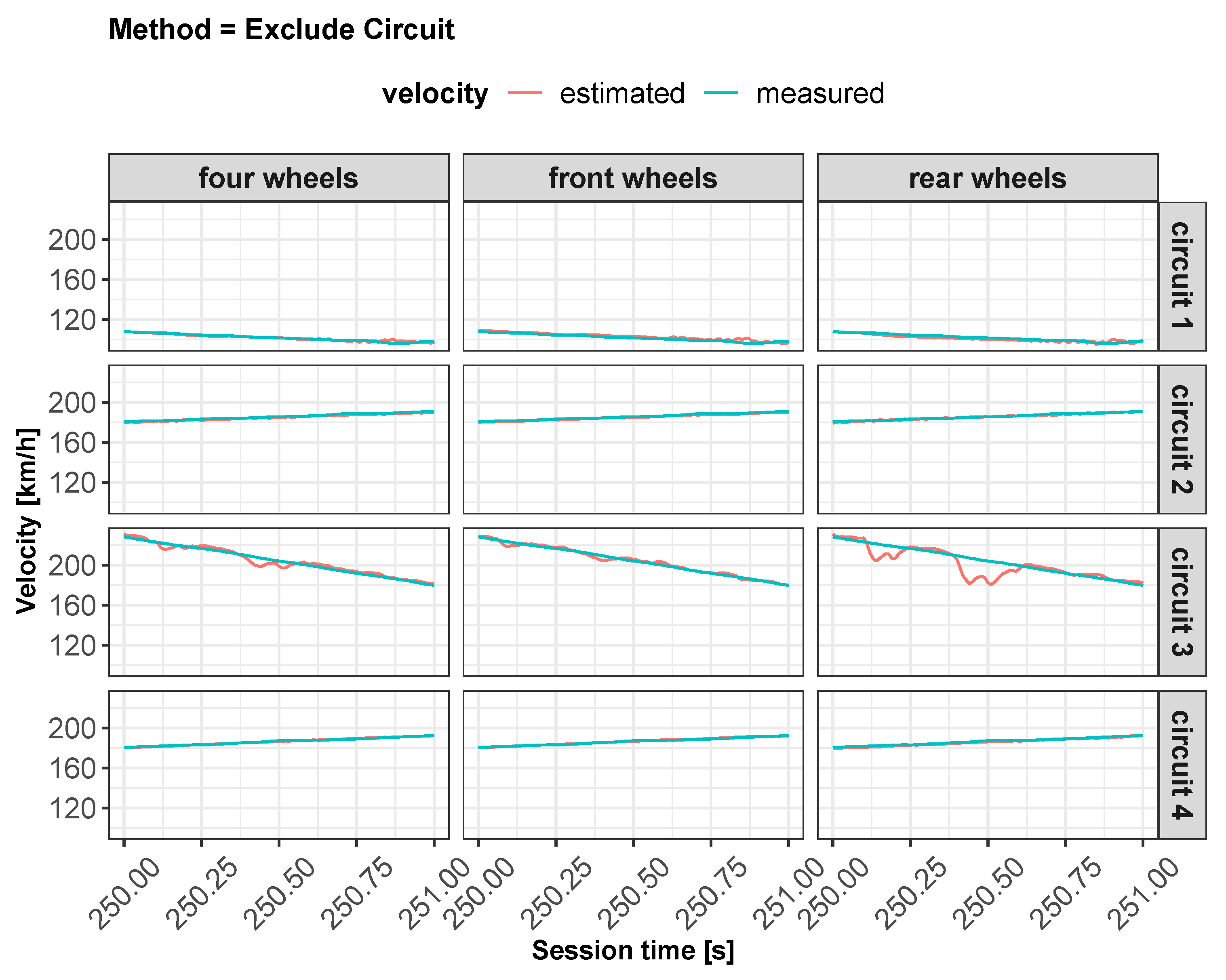
- Exclude: The neural network is trained with a set in which all data from a specific circuit or lap (either the first, intermediate or last one) are removed. These data are then used in the test set;
- Include: The neural network is trained with a set containing only data from a specific circuit or lap (either the first, intermediate or last one). These data are then excluded from the testing set.
3.6. Models’ Evaluation
- AIC (Akaike information criterion): The AIC, evaluated on a given dataset, is an indicator of the relative quality of the developed statistical models. Obtained via a series of different models for the data target, the AIC estimates the quality of each model relative to each of the other models. Thus, the AIC provides a mean for model selection [53].
- BIC (Bayesian information criterion): In statistics, the BIC or Schwarz criterion is a criterion for model selection among a finite set of models which is based, in part, on the likelihood function, and it is closely related to the AIC [54].
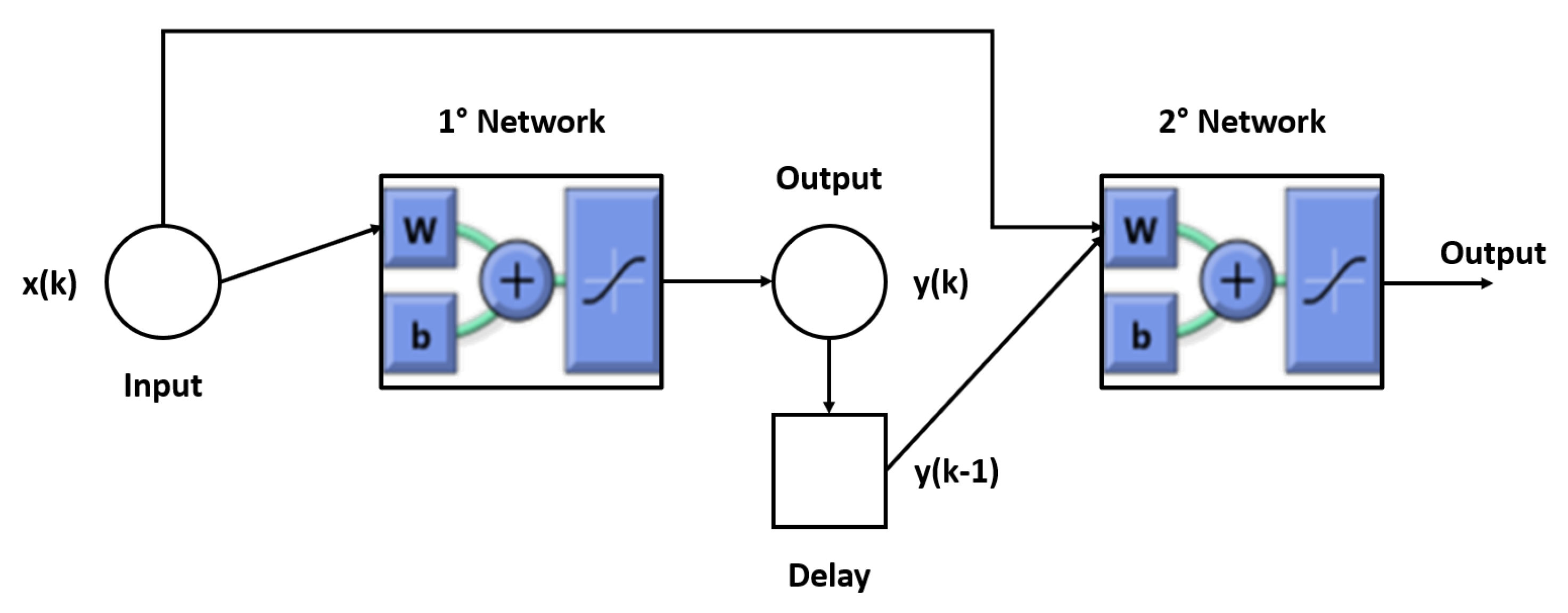
4. Improvements in Velocity Estimation through a Recurrent Neural Network-Based System
Design of Recurrent Neural Network
5. Results
5.1. Experimentation Results
- The “All” method shows a higher accuracy for each track because it involves a larger set of data, which includes data from all circuits, both for training and the testing phase;
- The “Exclude” circuit method shows a lower accuracy because, in such a case, the neural network is tested on a circuit not used for the testing phase so the different boundary conditions can alter the prediction;
- For each methodology, the highest error is registered for the artificial neural network configuration, which involved the rear wheels (i.e., driving wheels). This is caused by the highest value of slip being reached by the driving wheels, which allows the greatest accuracy. For the following considerations, a neural network that involved no-driving wheels has been considered.
5.2. Feed-Forward ANN KPIs Comparisons
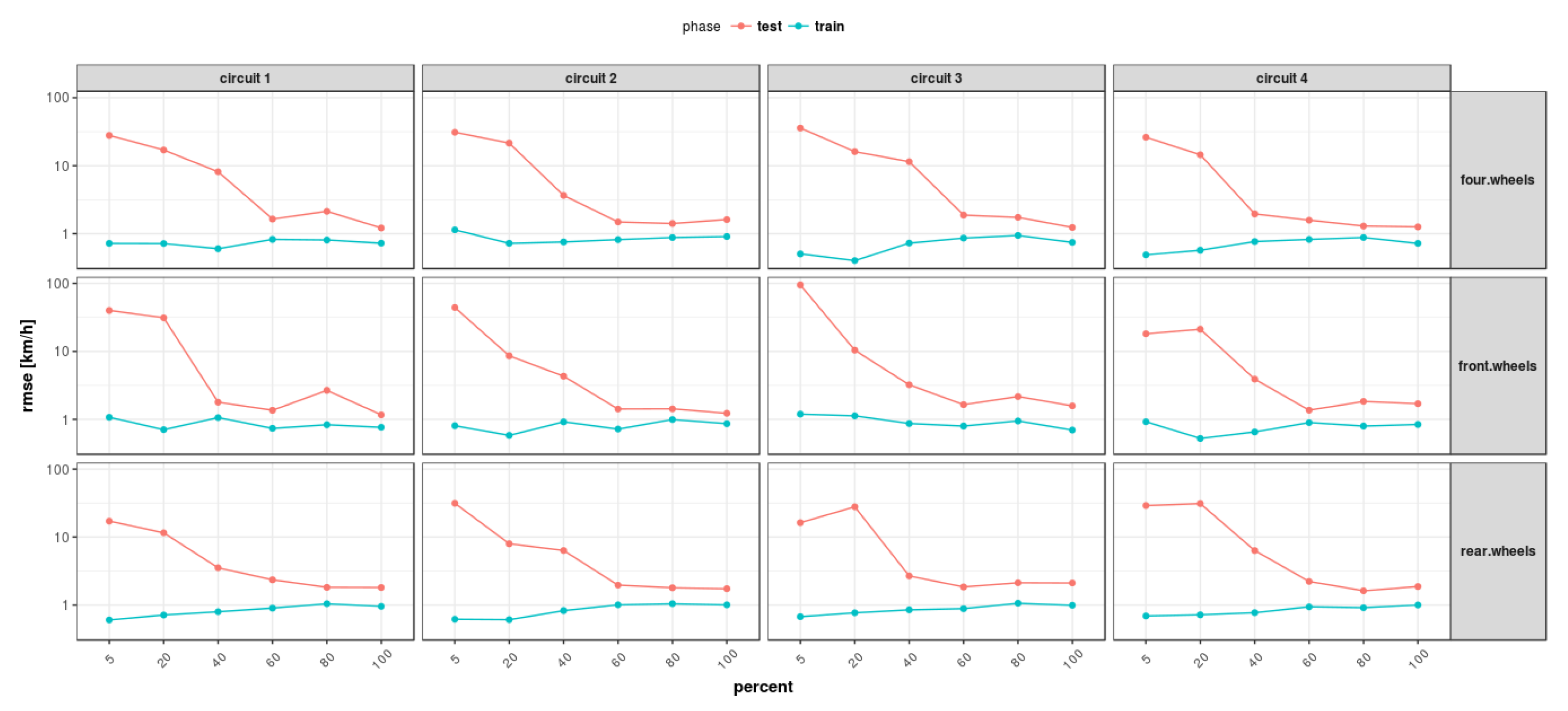
- By increasing the number of training samples after a certain value, the RMSE of the training phase increases as well due to an increase in the constraint condition numbers, which makes the training more difficult.
- Increasing the number of input samples produces an accuracy increment for the testing phase. It is important to notice that after a certain value of training samples, the RMSE of the testing phase reaches a horizontal asymptote.
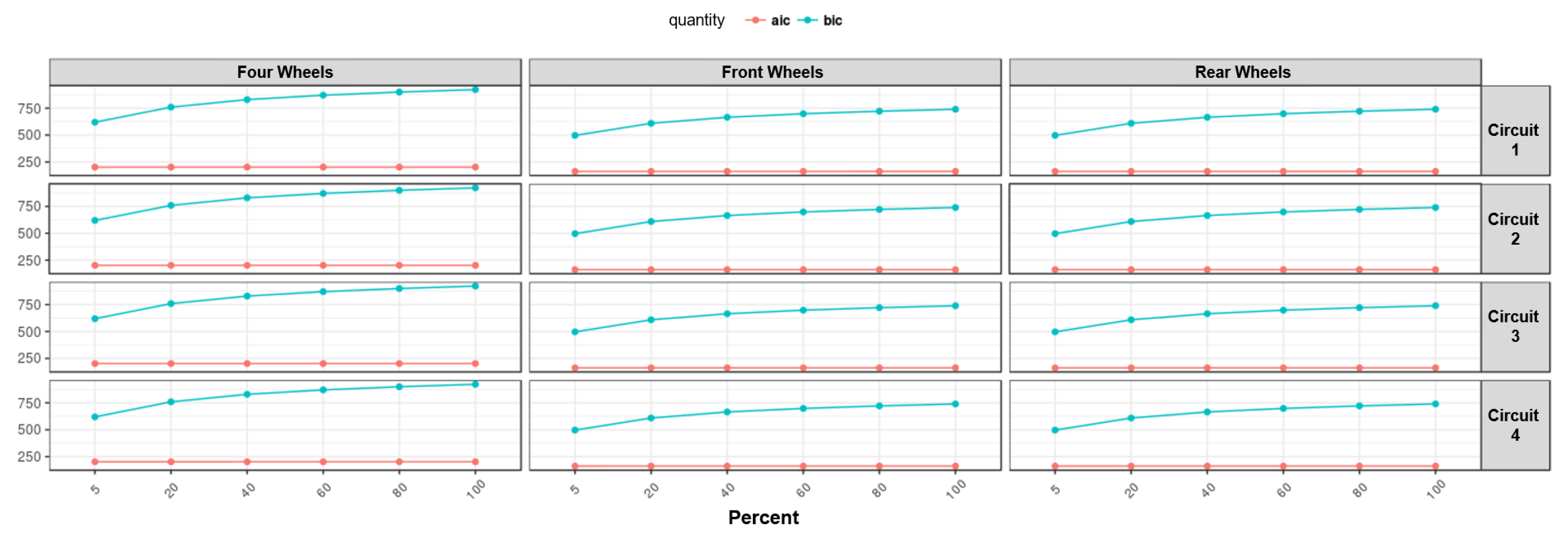
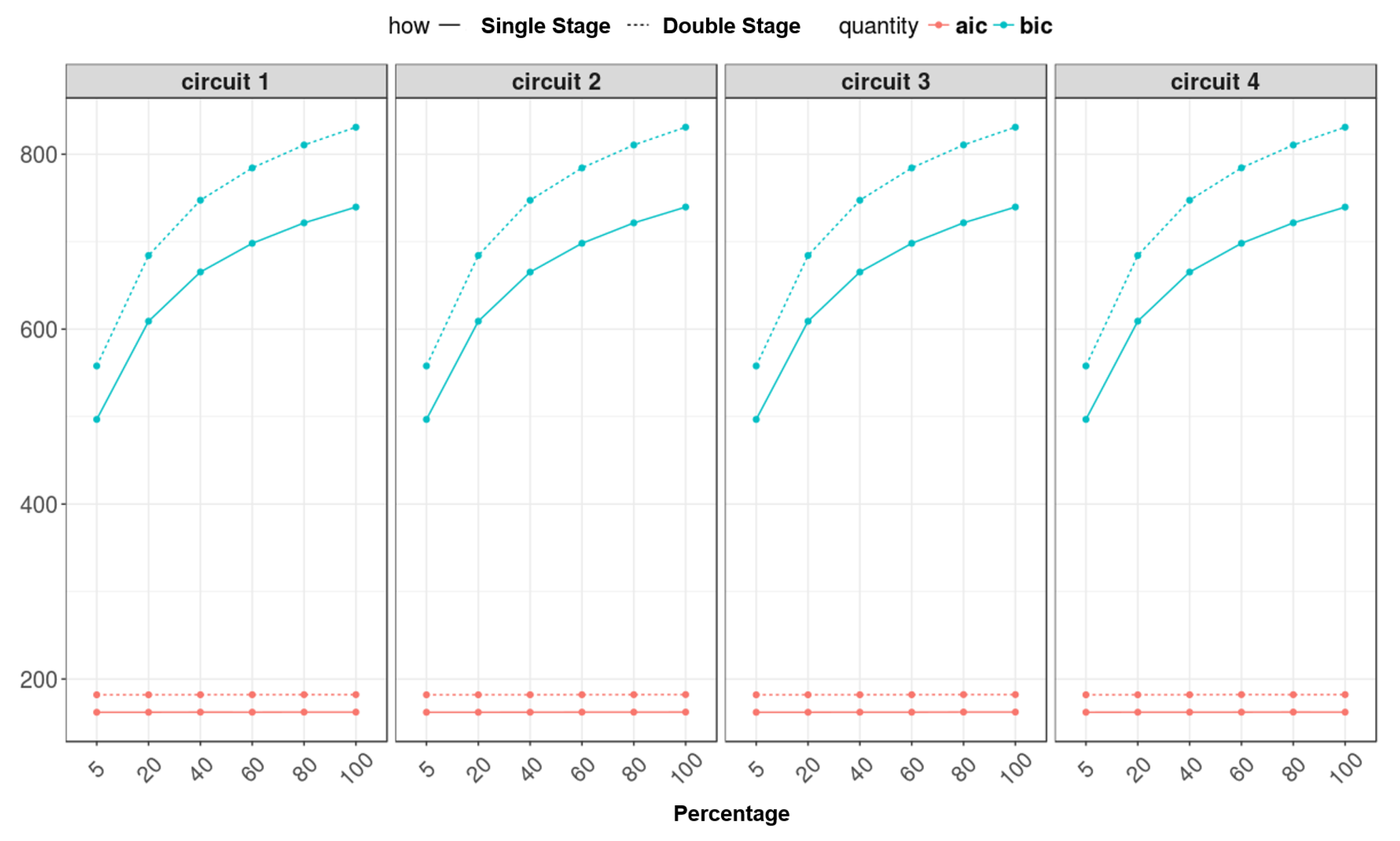
- The AIC and BIC parameters have higher values for the “four wheels” configuration, which involves more parameters, in accordance with what has been reported previously. By increasing the number of training samples, the AIC and BIC increase as well due to the increment of the constraining condition.
- Concerning the RMSE results, in accordance with what has been reported in the previous analysis, the highest error is registered for the artificial neural networks’ configuration involving the rear wheels (i.e., driving wheels).
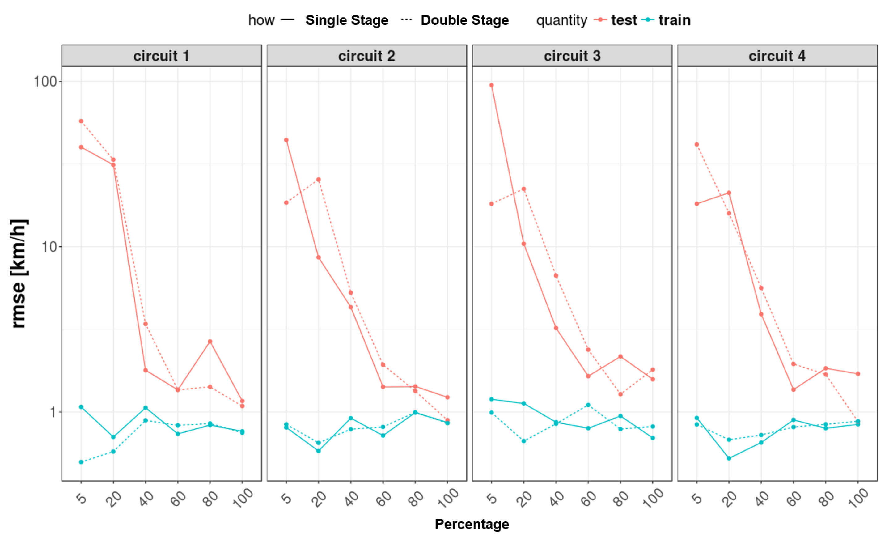
5.3. Feed-Forward and Recurrent Neural Network Comparison
6. Conclusions
Author Contributions
Funding
Institutional Review Board Statement
Informed Consent Statement
Data Availability Statement
Conflicts of Interest
References
- Leen, G.; Heffernan, D. Expanding automotive electronic systems. Computer 2002, 35, 88–93. [Google Scholar] [CrossRef]
- Walta, L.; Marchau, V.; Brookhuis, K. Stakeholder preferences of advanced driver assistance systems (ADAS)—A literature review. In Proceedings of the 13th World Congress and Exhibition on Intelligent Transport Systems and Service, London, UK, 8–12 October 2006. [Google Scholar]
- Tsourveloudis, N.C.; Valavanis, K.P.; Hebert, T. Autonomous vehicle navigation utilizing electrostatic potential fields and fuzzy logic. IEEE Trans. Robot. Autom. 2001, 17, 490–497. [Google Scholar] [CrossRef]
- Levinson, J.; Askeland, J.; Becker, J.; Dolson, J.; Held, D.; Kammel, S.; Kolter, J.Z.; Langer, D.; Pink, O.; Pratt, V.; et al. Towards fully autonomous driving: Systems and algorithms. In Proceedings of the 2011 IEEE Intelligent Vehicles Symposium (IV), Baden-Baden, Germany, 5–9 June 2011; pp. 163–168. [Google Scholar]
- Charette, R.N. This Car Runs on Code. IEEE Spectr. 2009, 46, 3. [Google Scholar]
- Ibañez-Guzmán, J.; Laugier, C.; Yoder, J.D.; Thrun, S. Autonomous Driving: Context and State-of-the-Art. In Handbook of Intelligent Vehicles; Springer: London, UK, 2012; pp. 1271–1310. [Google Scholar] [CrossRef]
- Jin, Y.; Ahn, H.; Kim, K.; Choi, S.; Mueck, M.; Frascolla, V.; Haustein, T. Adaptive automotive communications solutions of 10 years lifetime enabled by ETSI RRS software reconfiguration technology. In Proceedings of the Signal Processing Conference (EUSIPCO), 2017 25th European, Kos Island, Greece, 28 August–2 September 2017; pp. 903–906. [Google Scholar]
- Rajamani, R. Vehicle Dynamics and Control, 2nd ed.; Mechanical Engineering Series; Springer: Boston, MA, USA, 2012; p. 498. [Google Scholar] [CrossRef]
- Russo, R.; Terzo, M.; Timpone, F. Software-in-the-loop development and experimental testing of a semi-active magnetorheological coupling for 4WD on demand vehicles. In Proceedings of the Mini Conference Vehicle System Dynamics, Identification Anomalies (VSDIA 2008), Budapest, Hungary, 6–8 November 2008; pp. 73–82. [Google Scholar]
- Terzo, M.; Timpone, F. The control of the handling of a front wheel drive vehicle by means of a magnetorheological differential. Int. Rev. Mech. Eng. 2013, 7, 395–401. [Google Scholar]
- Santini, S.; Albarella, N.; Arricale, V.M.; Brancati, R.; Sakhnevych, A. On-board road friction estimation technique for autonomous driving vehicle-following maneuvers. Appl. Sci. 2021, 11, 2197. [Google Scholar] [CrossRef]
- Lefevre, S.; Laugier, C.; Ibanez-Guzman, J. Risk assessment at road intersections: Comparing intention and expectation. In Proceedings of the 2012 IEEE Intelligent Vehicles Symposium, Alcalá de Henares, Spain, 3–7 June 2012; pp. 165–171. [Google Scholar] [CrossRef]
- Short, M.; Pont, M. Hardware in the loop simulation of embedded automotive control system. In Proceedings of the 2005 IEEE Intelligent Transportation Systems Conference, Vienna, Austria, 16 September 2005; pp. 426–431. [Google Scholar] [CrossRef]
- Zhao, P.; Chen, J.; Mei, T.; Liang, H. Dynamic motion planning for autonomous vehicle in unknown environments. In Proceedings of the IEEE Intelligent Vehicles Symposium, Baden-Baden, Germany, 5–9 June 2011; pp. 284–289. [Google Scholar] [CrossRef]
- Ono, E.; Hattori, Y.; Muragishi, Y.; Koibuchi, K. Vehicle dynamics integrated control for four-wheel-distributed steering and four-wheel-distributed traction/braking systems. Veh. Syst. Dyn. 2006, 44, 139–151. [Google Scholar] [CrossRef]
- Halbach, S.; Sharer, P.; Pagerit, S.; Rousseau, A.P.; Folkerts, C. Model Architecture, Methods, and Interfaces for Efficient Math-Based Design and Simulation of Automotive Control Systems. In Proceedings of the SAE 2010 World Congress & Exhibition, Corning, NY, USA, 13 April 2010. [Google Scholar] [CrossRef]
- Farroni, F.; Sakhnevych, A.; Timpone, F. A three-dimensional multibody tire model for research comfort and handling analysis as a structural framework for a multi-physical integrated system. Proc. Inst. Mech. Eng. Part D J. Automob. Eng. 2018, 233, 0954407018799006. [Google Scholar] [CrossRef]
- Sakhnevych, A.; Arricale, V.M.; Bruschetta, M.; Censi, A.; Mion, E.; Picotti, E.; Frazzoli, E. Investigation on the model-based control performance in vehicle safety critical scenarios with varying tyre limits. Sensors 2021, 21, 5372. [Google Scholar] [CrossRef]
- Guiggiani, M. The Science of Vehicle Dynamics; Springer International Publishing: Cham, Switzerland, 2018. [Google Scholar] [CrossRef]
- Romano, L.; Sakhnevych, A.; Strano, S.; Timpone, F. A hybrid tyre model for in-plane dynamics. Veh. Syst. Dyn. 2019, 58, 1123–1145. [Google Scholar] [CrossRef]
- Romano, L.; Sakhnevych, A.; Strano, S.; Timpone, F. A novel brush-model with flexible carcass for transient interactions. Meccanica 2019, 54, 1663–1679. [Google Scholar] [CrossRef]
- Romano, L.; Timpone, F.; Bruzelius, F.; Jacobson, B. Analytical results in transient brush tyre models: Theory for large camber angles and classic solutions with limited friction. Meccanica 2022, 57, 165–191. [Google Scholar] [CrossRef]
- Villano, E.; Lenzo, B.; Sakhnevych, A. Cross-combined UKF for vehicle sideslip angle estimation with a modified Dugoff tire model: Design and experimental results. Meccanica 2021, 56, 2653–2668. [Google Scholar] [CrossRef]
- Coppola, L.; De Marco, B.; Niola, V.; Sakhnevych, A.; Timpone, F. Impact attenuator optimum design for a FSAE racing car by numerical and experimental crash analysis. Int. J. Automot. Technol. 2020, 21, 1339–1348. [Google Scholar] [CrossRef]
- Jiang, F.; Gao, Z. An adaptive nonlinear filter approach to the vehicle velocity estimation for ABS. In Proceedings of the 2000 IEEE International Conference on Control Applications. Conference Proceedings (Cat. No.00CH37162), Anchorage, AK, USA, 27 September 2000; pp. 490–495. [Google Scholar] [CrossRef]
- Guofu, L. ABS system is based on data fusion technology, the speed estimation method. J. Sci. Instrum. 2004, 29, 736–765. [Google Scholar]
- Zhao, L.; Liu, Z.; Chen, H. Sliding mode observer for vehicle velocity estimation with road grade and bank angles adaptation. In Proceedings of the 2009 IEEE Intelligent Vehicles Symposium, Xi’an, China, 3–5 June 2009; pp. 701–706. [Google Scholar] [CrossRef]
- Chu, L.; Shi, Y.; Zhang, Y.; Liu, H.; Xu, M. Vehicle lateral and longitudinal velocity estimation based on Adaptive Kalman Filter. In Proceedings of the 2010 3rd International Conference on Advanced Computer Theory and Engineering(ICACTE), Chengdu, China, 20–22 August 2010; Volume 3, pp. V3-325–V3-329. [Google Scholar] [CrossRef]
- Villagra, J.; d’Andrea Novel, B.; Fliess, M.; Mounier, H. Estimation of longitudinal and lateral vehicle velocities: An algebraic approach. In Proceedings of the 2008 American Control Conference, Seattle, WA, USA, 11–13 June 2008; pp. 3941–3946. [Google Scholar] [CrossRef]
- Best, M.; Gordon, T.; Dixon, P. An Extended Adaptive Kalman Filter for Real-time State Estimation of Vehicle Handling Dynamics. Veh. Syst. Dyn. 2000, 34, 57–75. [Google Scholar] [CrossRef]
- Daiss, A.; Kiencke, U. Estimation of vehicle speed fuzzy-estimation in comparison with Kalman-filtering. In Proceedings of the International Conference on Control Applications, Seattle, WA, USA, 21–23 June 1995; pp. 281–284. [Google Scholar] [CrossRef]
- Song, C.K.; Uchanski, M.; Karl Hedrick, J. Vehicle Speed Estimation Using Accelerometer and Wheel Speed Measurements. In Proceedings of the International Body Engineering Conference & Exhibition and Automotive & Transportation Technology Congress, Paris, France, 9 July 2002. [Google Scholar] [CrossRef]
- Jaballah, B.; M’Sirdi, N.K.; Naamane, A.; Messaoud, H. Estimation of longitudinal and lateral velocity of vehicle. In Proceedings of the 2009 17th Mediterranean Conference on Control and Automation, Thessaloniki, Greece, 24–26 June 2009; pp. 582–587. [Google Scholar] [CrossRef]
- Hsu, L.Y.; Chen, T.L. Vehicle Full-State Estimation and Prediction System Using State Observers. IEEE Trans. Veh. Technol. 2009, 58, 2651–2662. [Google Scholar] [CrossRef]
- Farrelly, J.; Wellstead, P. Estimation of vehicle lateral velocity. In Proceedings of the 1996 IEEE International Conference on Control Applications held Together with IEEE International Symposium on Intelligent Contro, Dearborn, MI, USA, 15–18 September 1996; pp. 552–557. [Google Scholar] [CrossRef]
- Hunt, K.J.; Irwin, G.R.; Warwick, K. Neural Network Engineering in Dynamic Control Systems; Advances in Industrial Control; Springer: London, UK, 1995. [Google Scholar] [CrossRef]
- Lee, J. Measurement of machine performance degradation using a neural network model. Comput. Ind. 1996, 30, 193–209. [Google Scholar] [CrossRef]
- Zhai, Y.J.; Yu, D.L. Neural network model-based automotive engine air/fuel ratio control and robustness evaluation. Eng. Appl. Artif. Intell. 2009, 22, 171–180. [Google Scholar] [CrossRef]
- Meijer, G.C. Smart Sensor Systems; John Wiley & Sons, Ltd.: Chichester, UK, 2008. [Google Scholar] [CrossRef]
- Jurgen, R.K. Electronic Engine Control Technologies; SAE International: Warrendale, PN, USA, 2004. [Google Scholar]
- Marko, K.; James, J.; Dosdall, J.; Murphy, J. Automotive control system diagnostics using neural nets for rapid pattern classification of large data sets. In Proceedings of the 1989 International Joint Conference on Neural Networks, Washington, DC, USA, 19–22 June 1989; Volume 13, p. 16. [Google Scholar]
- Puskorius, G.V.; Feldkamp, L.A. Neurocontrol of nonlinear dynamical systems with Kalman filter trained recurrent networks. IEEE Trans. Neural Netw. 1994, 5, 279–297. [Google Scholar] [CrossRef]
- Walczak, S.; Cerpa, N. Heuristic principles for the design of artificial neural networks. Inf. Softw. Technol. 1999, 41, 107–117. [Google Scholar] [CrossRef]
- Li, Z.; Wang, D.; Kang, Q. The Development of Data Acquisition System of Formula SAE Race Car Based on CAN Bus Communication Interface and Closed-Loop Design of Racing Car. Wirel. Commun. Mob. Comput. 2021, 2021, 4211010. [Google Scholar] [CrossRef]
- De Martino, M.; Farroni, F.; Pasquino, N.; Sakhnevych, A.; Timpone, F. Real-time estimation of the vehicle sideslip angle through regression based on principal component analysis and neural networks. In Proceedings of the 2017 IEEE International Systems Engineering Symposium, Vienna, Austria, 11–13 October 2017; pp. 1–6. [Google Scholar] [CrossRef]
- Lippmann, R. An introduction to computing with neural nets. IEEE ASSP Mag. 1987, 4, 4–22. [Google Scholar] [CrossRef]
- Yu, Y.; Si, X.; Hu, C.; Zhang, J. A review of recurrent neural networks: LSTM cells and network architectures. Neural Comput. 2019, 31, 1235–1270. [Google Scholar] [CrossRef]
- Goldberg, D.E.; Holland, J.H. Genetic Algorithms and Machine Learning. Mach. Learn. 1988, 3, 95–99. [Google Scholar] [CrossRef]
- Sola, J.; Sevilla, J. Importance of input data normalization for the application of neural networks to complex industrial problems. IEEE Trans. Nucl. Sci. 1997, 44, 1464–1468. [Google Scholar] [CrossRef]
- Csáji, B.C. Approximation with artificial neural networks. Fac. Sci. Etvs. Lornd. Univ. Hung. 2001, 24, 48. [Google Scholar]
- Igel, C.; Hüsken, M. Improving the Rprop learning algorithm. In Proceedings of the Second International ymposium Neural Computer, NC’2000, Berlin, Germany, 23–26 May 2000. [Google Scholar]
- Connor, J.T.; Martin, R.D.; Atlas, L.E. Recurrent Neural Networks and Robust Time Series Prediction. IEEE Trans. Neural Netw. 1994, 5, 279188. [Google Scholar] [CrossRef]
- Portet, S. A primer on model selection using the Akaike Information Criterion. Infect. Dis. Model. 2020, 5, 111–128. [Google Scholar] [CrossRef]
- Chen, S.S.; Gopalakrishnan, P. Clustering via the Bayesian information criterion with applications in speech recognition. In Proceedings of the 1998 IEEE International Conference Acoustics, Speech and Signal Process, ICASSP ’98 (Cat. No.98CH36181), Seattle, WA, USA, 15 May 1998; Volume 2, pp. 645–648. [Google Scholar] [CrossRef]
- Farroni, F. TRICK-Tire/Road Interaction Characterization & Knowledge-A tool for the evaluation of tire and vehicle performances in outdoor test sessions. Mech. Syst. Signal Process. 2016, 72, 808–831. [Google Scholar]


Publisher’s Note: MDPI stays neutral with regard to jurisdictional claims in published maps and institutional affiliations. |
© 2022 by the authors. Licensee MDPI, Basel, Switzerland. This article is an open access article distributed under the terms and conditions of the Creative Commons Attribution (CC BY) license (https://creativecommons.org/licenses/by/4.0/).
Share and Cite
Napolitano Dell’Annunziata, G.; Arricale, V.M.; Farroni, F.; Genovese, A.; Pasquino, N.; Tranquillo, G. Estimation of Vehicle Longitudinal Velocity with Artificial Neural Network. Sensors 2022, 22, 9516. https://doi.org/10.3390/s22239516
Napolitano Dell’Annunziata G, Arricale VM, Farroni F, Genovese A, Pasquino N, Tranquillo G. Estimation of Vehicle Longitudinal Velocity with Artificial Neural Network. Sensors. 2022; 22(23):9516. https://doi.org/10.3390/s22239516
Chicago/Turabian StyleNapolitano Dell’Annunziata, Guido, Vincenzo Maria Arricale, Flavio Farroni, Andrea Genovese, Nicola Pasquino, and Giuseppe Tranquillo. 2022. "Estimation of Vehicle Longitudinal Velocity with Artificial Neural Network" Sensors 22, no. 23: 9516. https://doi.org/10.3390/s22239516
APA StyleNapolitano Dell’Annunziata, G., Arricale, V. M., Farroni, F., Genovese, A., Pasquino, N., & Tranquillo, G. (2022). Estimation of Vehicle Longitudinal Velocity with Artificial Neural Network. Sensors, 22(23), 9516. https://doi.org/10.3390/s22239516