
Machine Learning-Based Ensemble Classifiers for Anomaly Handling in Smart Home Energy Consumption Data
 ,
,  ,
,  and
and 
Abstract
1. Introduction
- ▪
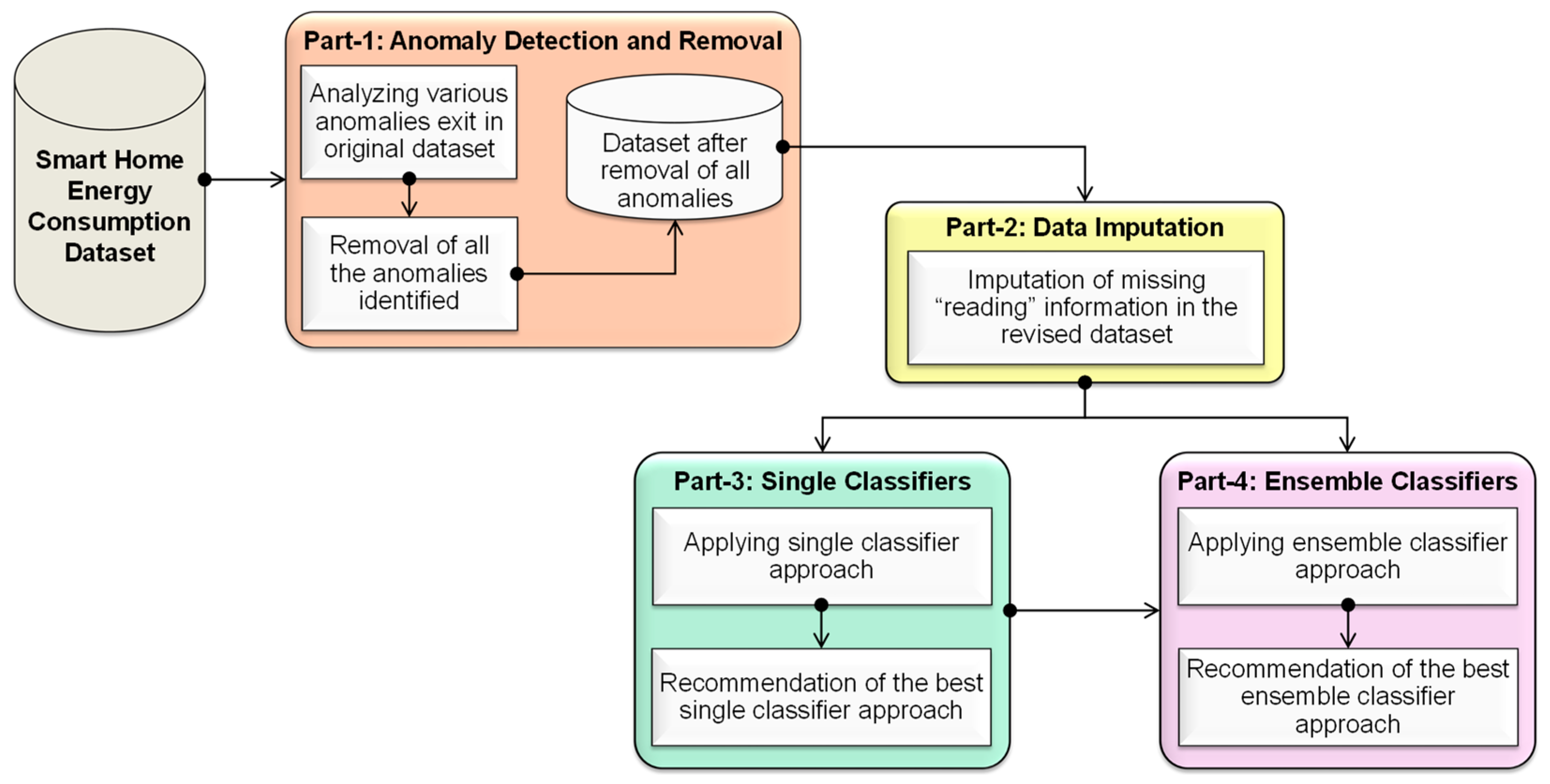
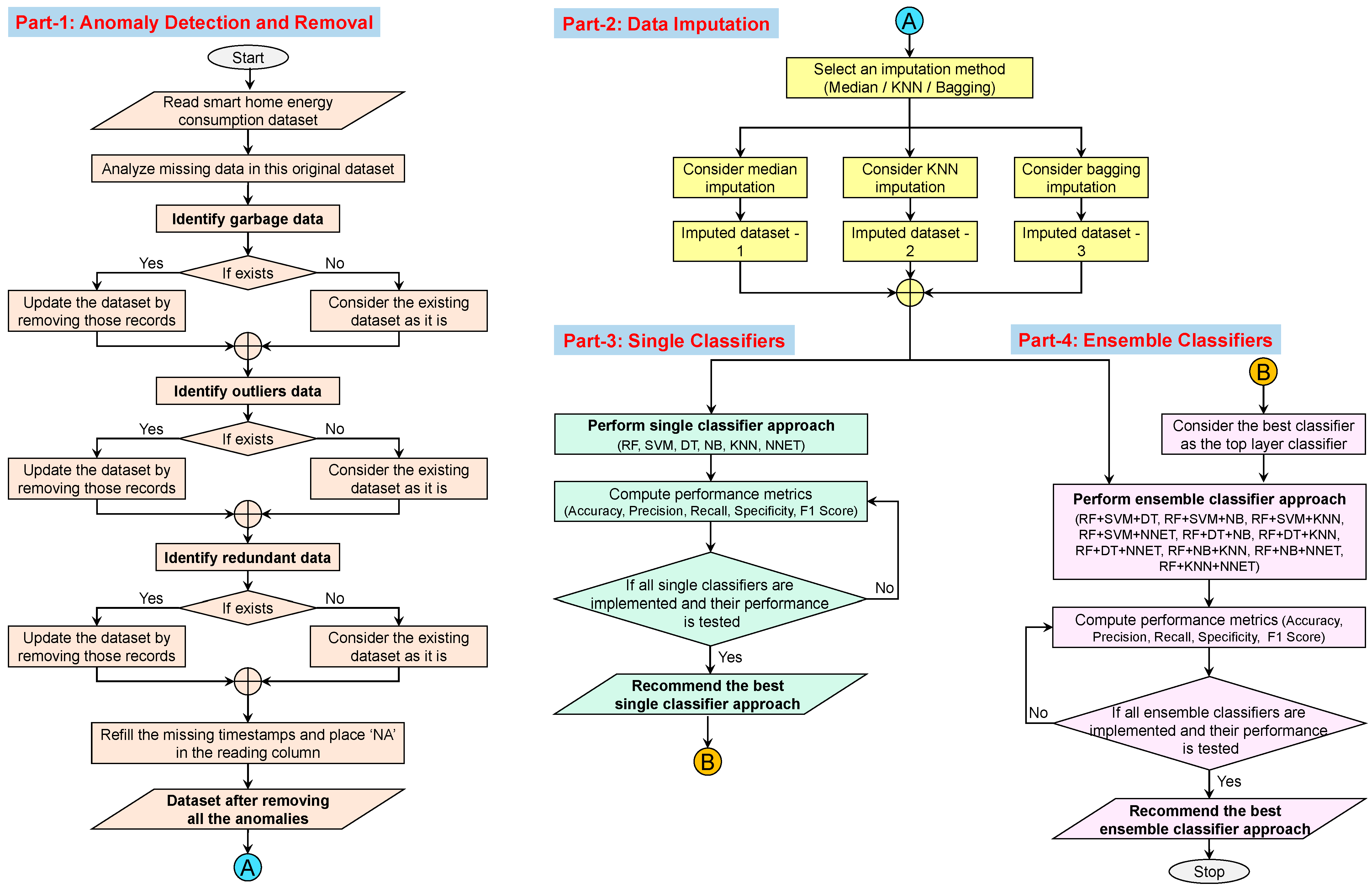
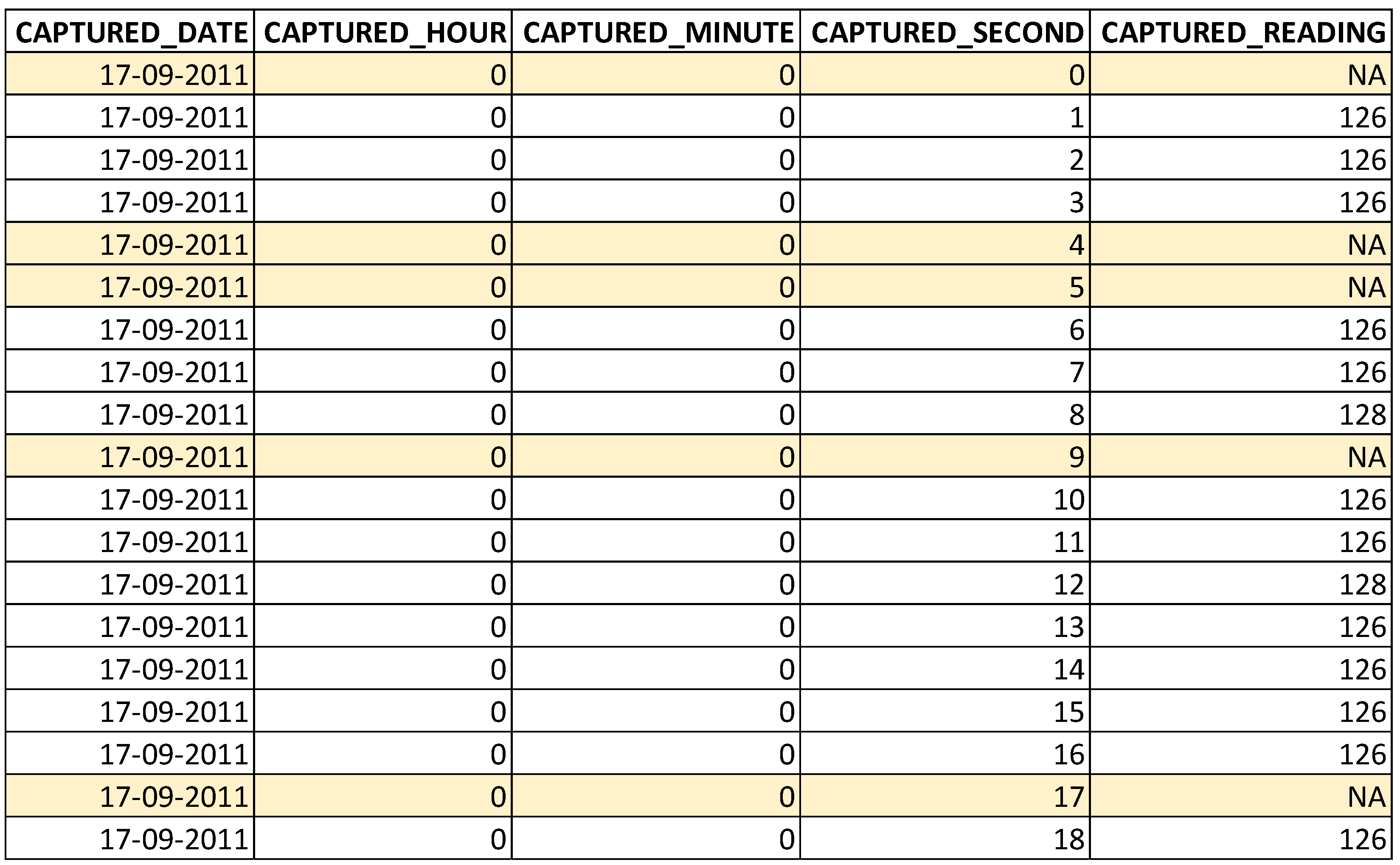
- The proposed approach initially identifies all anomalies and removes them, and then imputes this information. The entire implementation consists of four parts.
- -
- Part 1 (anomaly detection and removal) considers the original dataset and refines it by removing all the identified anomalies.
- -
- Part 2 (data imputation) considers this refined dataset and performs the missing data imputation using median, KNN, and bagging imputation methods, thereby producing an anomaly-free dataset.
- -
- Part 3 (single-classifier approaches) performs the classification of the dataset using the conventional single-classifier approaches such as RF, SVM, DT, NB, KNN, and NNET.
- -
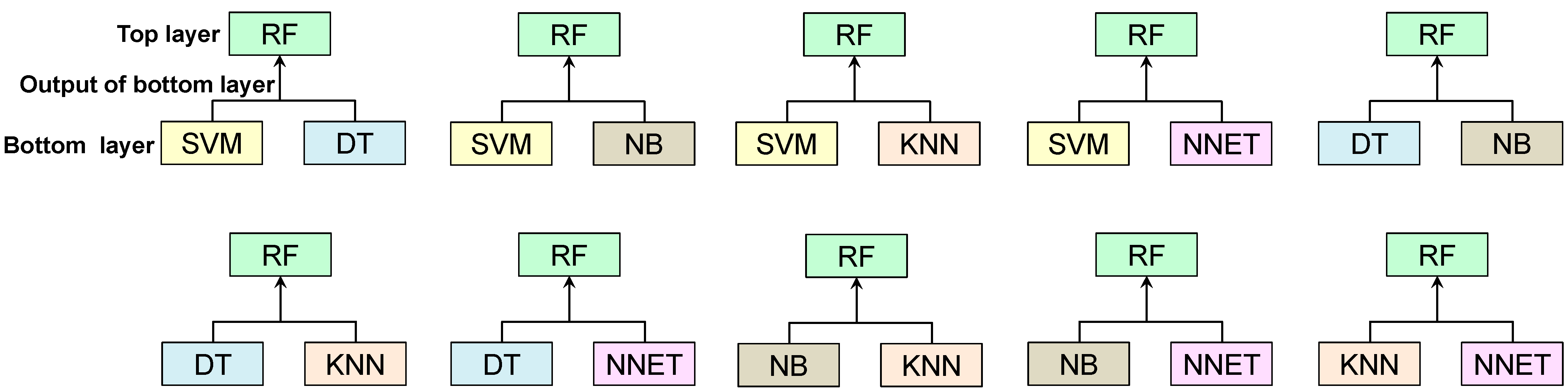
- Part 4 (ensemble classifiers approaches) performs the classification of the dataset using the proposed ensemble classifier approaches such as RF+SVM+DT, RF+SVM+NB, RF+SVM+KNN, RF+SVM+NNET, RF+DT+NB, RF+DT+KNN, RF+DT+NNET, RF+NB+KNN, RF+NB+NNET, and RF+KNN+NNET.
- ▪
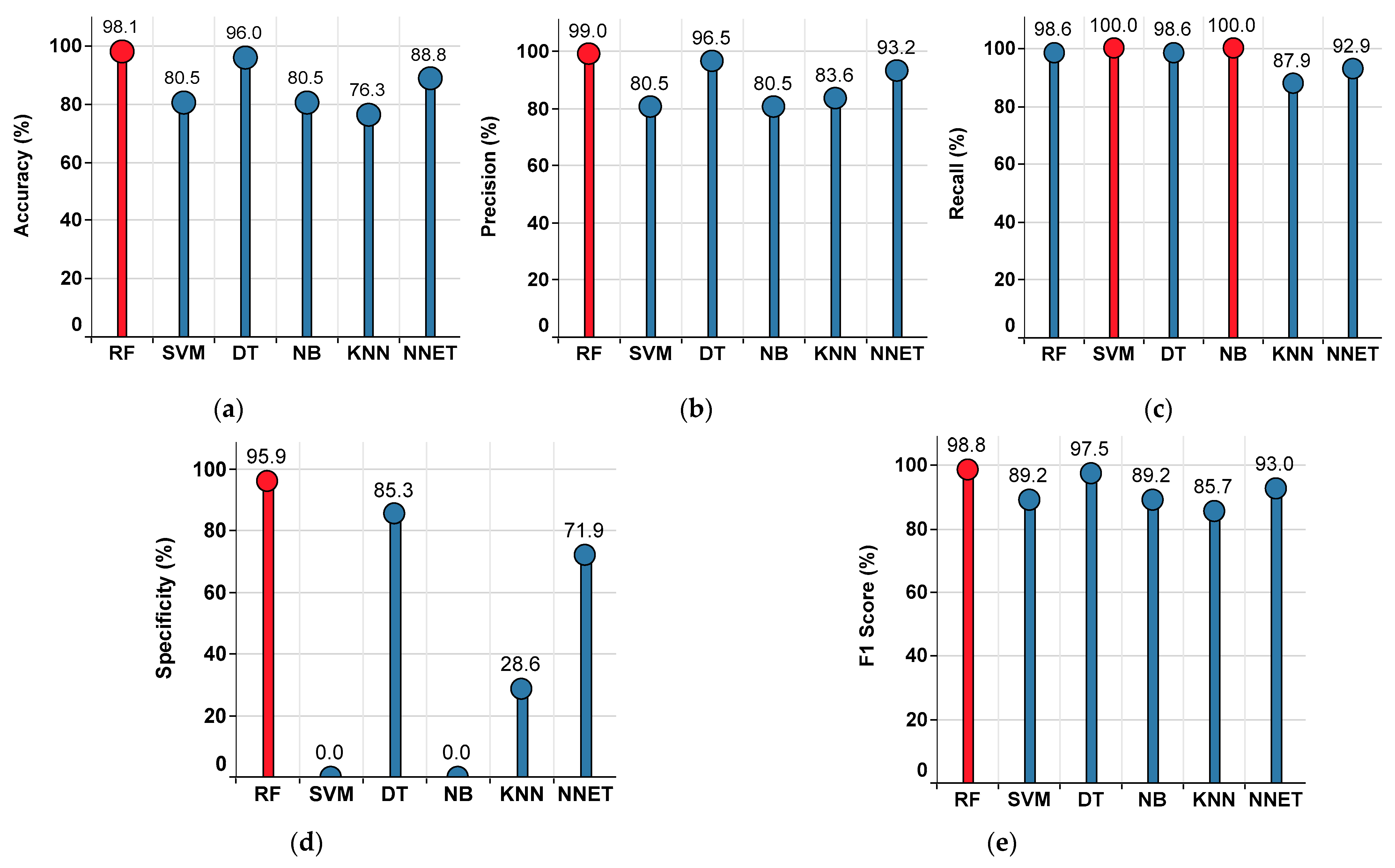
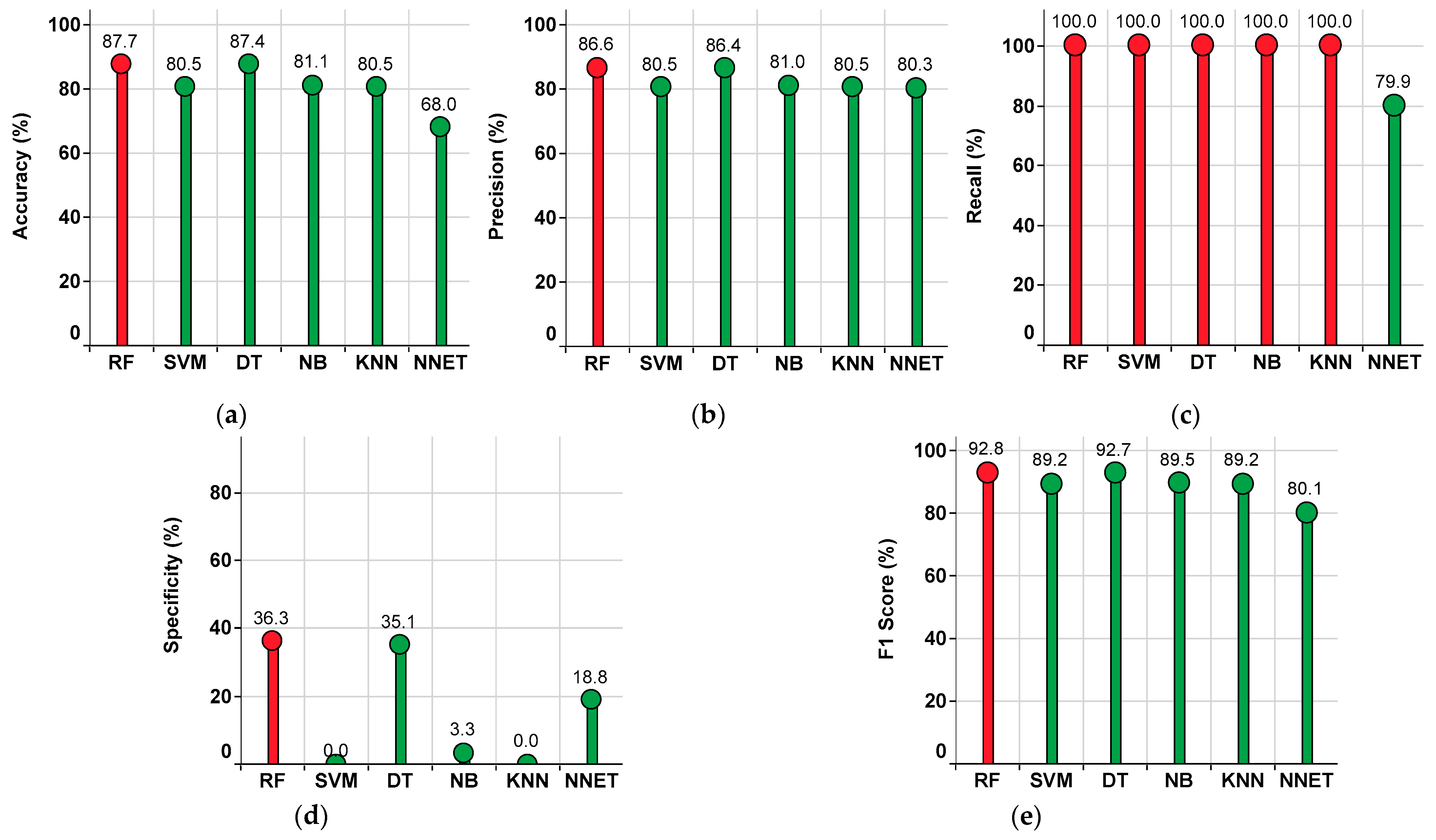
- To assess the classifiers’ performance, various metrics, namely, accuracy, precision, recall/sensitivity, specificity, and F1 score are computed. From these metrics, it is identified that the ensemble classifier “RF+SVM+DT” has shown superior performance over the conventional single classifiers as well the other ensemble classifiers for anomaly handling in smart home energy consumption data.
2. Description of Dataset
3. Description and Implementation of the Proposed Approach
3.1. Implementation of Part 1 (Anomaly Detection and Removal)
3.2. Implementation of Part 2 (Data Imputation)
3.2.1. Implementation of the Median Imputation Method
3.2.2. Implementation of the KNN Imputation Method
3.2.3. Implementation of the Bagging Imputation Method
3.3. Implementation of Part 3 (Single-Classifier Approach)
3.4. Implementation of Part 4 (Ensemble Classifiers Approach)
4. Simulation Results and Discussion
4.1. Results Corresponding to Anomaly Detection and Removal
4.2. Results Corresponding to the Single-Classifier Approach
4.2.1. Performance of the Single-Classifier Approach in the Median Imputation Method
4.2.2. Performance of the Single-Classifier Approach in the KNN Imputation Method
4.2.3. Performance of the Single-Classifier Approach in the Bagging Imputation Method
4.3. Results Corresponding to the Ensemble Classifiers Approach
4.3.1. Performance of the Ensemble Classifiers Approach in the Median Imputation Method
4.3.2. Performance of the Ensemble Classifiers Approach in the KNN Imputation Method
4.3.3. Performance of the Ensemble Classifiers Approach in the Bagging Imputation Method
5. Conclusions
- ▪
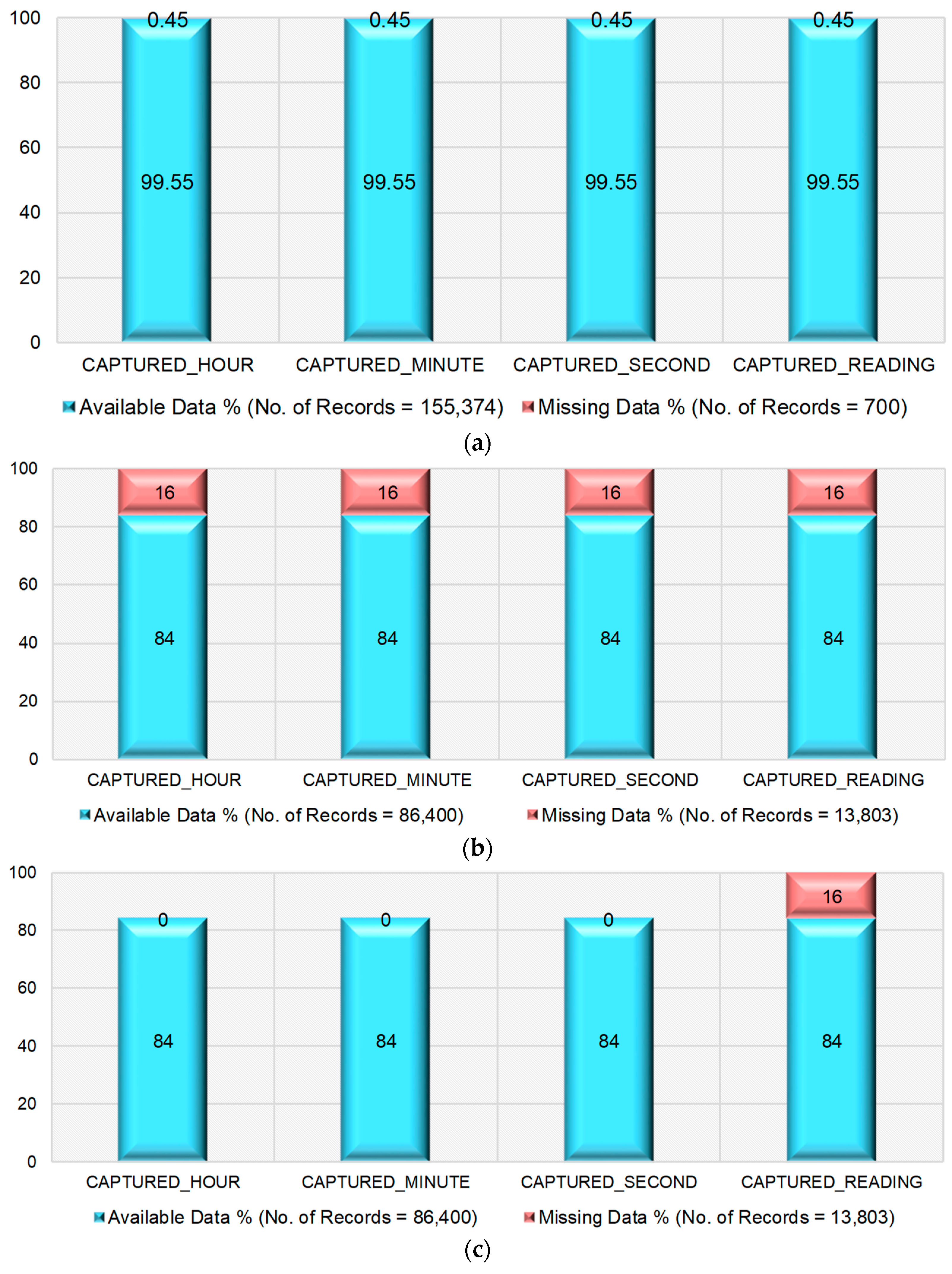
- All the possible anomalies are successfully identified and removed from the dataset. The number of records in the original dataset is 155,374 and the number of records available in the refined dataset after removing anomalies is 86,400, which is the actual expected number of records as per the dataset description.
- ▪
- Out of 86,400 records, 13,803 records are identified as records with missing data. This missing data has been successfully imputed by using various imputation methods (median, KNN, and bagging).
- ▪
- To assess the process of imputation, various conventional single-classifier approaches, as well as the proposed ensemble classifiers approaches, are implemented. From the computation of the performance metrics (accuracy, precision, recall/sensitivity, specificity, and F1 score), the RF classifier is identified as the superior single-classifier to all other single classifiers.
- ▪
- Out of the proposed ensemble classifiers, “RF+SVM+DT” has shown superior performance over the conventionally best single classifier (RF) as well the other ensemble classifiers for imputing the missing reading information.
Impacts and Implications of the Work
Author Contributions
Funding
Institutional Review Board Statement
Informed Consent Statement
Data Availability Statement
Acknowledgments
Conflicts of Interest
Abbreviations
| CSV | comma-separated values |
| DT | decision tree |
| KNN | K-nearest neighbour |
| ML | machine learning |
| MICE | multivariate imputation by chained equations |
| NA | not available |
| NB | naive Bayes |
| NILM | non-intrusive load monitoring |
| NNET | neural networks |
| RF | random forest |
| SVM | support vector machine |
References
- Firmani, D.; Mecella, M.; Scannapieco, M.; Batini, C. On the Meaningfulness of “Big Data Quality”. Data Sci. Eng. 2016, 1, 6–20. [Google Scholar] [CrossRef]
- Chen, W.; Zhou, K.; Yang, S.; Wu, C. Data Quality of Electricity Consumption Data in a Smart Grid Environment. Renew. Sustain. Energy Rev. 2017, 75, 98–105. [Google Scholar] [CrossRef]
- Tu, C.; He, X.; Shuai, Z.; Jiang, F. Big Data Issues in Smart Grid—A Review. Renew. Sustain. Energy Rev. 2017, 79, 1099–1107. [Google Scholar] [CrossRef]
- Ghorbanian, M.; Dolatabadi, S.H.; Siano, P. Big Data Issues in Smart Grids: A Survey. IEEE Syst. J. 2019, 13, 4158–4168. [Google Scholar] [CrossRef]
- Bhattarai, B.P.; Paudyal, S.; Luo, Y.; Mohanpurkar, M.; Cheung, K.; Tonkoski, R.; Hovsapian, R.; Myers, K.S.; Zhang, R.; Zhao, P.; et al. Big Data Analytics in Smart Grids: State-of-the-art, Challenges, Opportunities, and Future Directions. IET Smart Grid 2019, 2, 141–154. [Google Scholar] [CrossRef]
- Kasaraneni, P.P.; Yellapragada, V.P.K. Simple and Effective Descriptive Analysis of Missing Data Anomalies in Smart Home Energy Consumption Readings. J. Energy Syst. 2021, 5, 199–220. [Google Scholar] [CrossRef]
- Kasaraneni, P.P.; Yellapragada Venkata, P.K. Analytical Approach to Exploring the Missing Data Behavior in Smart Home Energy Consumption Dataset. J. Renew. Energy Environ. 2022, 9, 37–48. [Google Scholar] [CrossRef]
- Kasaraneni, P.P.; Yellapragada, V.P.K. Systematic Statistical Analysis to Ascertain the Missing Data Patterns in Energy Consumption Data of Smart Homes. Int. J. Renew. Energy Res. 2022, 12, 1560–1573. [Google Scholar] [CrossRef]
- Emmanuel, T.; Maupong, T.; Mpoeleng, D.; Semong, T.; Mphago, B.; Tabona, O. A Survey on Missing Data in Machine Learning. J. Big Data 2021, 8, 140. [Google Scholar] [CrossRef]
- Jäger, S.; Allhorn, A.; Bießmann, F. A Benchmark for Data Imputation Methods. Front. Big Data 2021, 4, 693674. [Google Scholar] [CrossRef]
- Dimitris, B.; Pawlowski, C.; Ying, D.Z. From Predictive Methods to Missing Data Imputation: An Optimization Approach. J. Mach. Learn. Res. 2018, 18, 1–39. Available online: https://jmlr.csail.mit.edu/papers/volume18/17-073/17-073.pdf (accessed on 2 November 2022).
- Alabadla, M.; Sidi, F.; Ishak, I.; Ibrahim, H.; Affendey, L.S.; Che Ani, Z.; Jabar, M.A.; Bukar, U.A.; Devaraj, N.K.; Muda, A.S.; et al. Systematic Review of Using Machine Learning in Imputing Missing Values. IEEE Access 2022, 10, 44483–44502. [Google Scholar] [CrossRef]
- Wu, R.; Hamshaw, S.D.; Yang, L.; Kincaid, D.W.; Etheridge, R.; Ghasemkhani, A. Data Imputation for Multivariate Time Series Sensor Data with Large Gaps of Missing Data. IEEE Sens. J. 2022, 22, 10671–10683. [Google Scholar] [CrossRef]
- Jiang, X.; Tian, Z.; Li, K. A Graph-Based Approach for Missing Sensor Data Imputation. IEEE Sens. J. 2021, 21, 23133–23144. [Google Scholar] [CrossRef]
- Weber, M.; Turowski, M.; Cakmak, H.K.; Mikut, R.; Kuhnapfel, U.; Hagenmeyer, V. Data-Driven Copy-Paste Imputation for Energy Time Series. IEEE Trans. Smart Grid 2021, 12, 5409–5419. [Google Scholar] [CrossRef]
- Jeong, D.; Park, C.; Ko, Y.M. Missing Data Imputation Using Mixture Factor Analysis for Building Electric Load Data. Appl. Energy 2021, 304, 117655. [Google Scholar] [CrossRef]
- Okafor, N.U.; Delaney, D.T. Missing Data Imputation on IoT Sensor Networks: Implications for on-Site Sensor Calibration. IEEE Sens. J. 2021, 21, 22833–22845. [Google Scholar] [CrossRef]
- Bhagat, H.V.; Singh, M. NMVI: A Data-Splitting Based Imputation Technique for Distinct Types of Missing Data. Chemom. Intell. Lab. Syst. 2022, 223, 104518. [Google Scholar] [CrossRef]
- Su, T.; Shi, Y.; Yu, J.; Yue, C.; Zhou, F. Nonlinear Compensation Algorithm for Multidimensional Temporal Data: A Missing Value Imputation for the Power Grid Applications. Knowl.-Based Syst. 2021, 215, 106743. [Google Scholar] [CrossRef]
- Jurado, S.; Nebot, À.; Mugica, F.; Mihaylov, M. Fuzzy Inductive Reasoning Forecasting Strategies Able to Cope with Missing Data: A Smart Grid Application. Appl. Soft Comput. 2017, 51, 225–238. [Google Scholar] [CrossRef]
- Hemanth, G.R.; Charles Raja, S. Proposing Suitable Data Imputation Methods by Adopting a Stage Wise Approach for Various Classes of Smart Meters Missing Data—Practical Approach. Expert Syst. Appl. 2022, 187, 115911. [Google Scholar] [CrossRef]
- Ryu, S.; Kim, M.; Kim, H. Denoising Autoencoder-Based Missing Value Imputation for Smart Meters. IEEE Access 2020, 8, 40656–40666. [Google Scholar] [CrossRef]
- Le, N.T.; Benjapolakul, W. A Data Imputation Model in Phasor Measurement Units Based on Bagged Averaging of Multiple Linear Regression. IEEE Access 2018, 6, 39324–39333. [Google Scholar] [CrossRef]
- Liu, X.; Zhang, Z. A Two-Stage Deep Autoencoder-Based Missing Data Imputation Method for Wind Farm SCADA Data. IEEE Sens. J. 2021, 21, 10933–10945. [Google Scholar] [CrossRef]
- Andiojaya, A.; Demirhan, H. A Bagging Algorithm for the Imputation of Missing Values in Time Series. Expert Syst. Appl. 2019, 129, 10–26. [Google Scholar] [CrossRef]
- Choudhury, S.J.; Pal, N.R. Imputation of Missing Data with Neural Networks for Classification. Knowl. Based Syst. 2019, 182, 104838. [Google Scholar] [CrossRef]
- Sim, J.; Lee, J.S.; Kwon, O. Missing Values and Optimal Selection of an Imputation Method and Classification Algorithm to Improve the Accuracy of Ubiquitous Computing Applications. Math. Probl. Eng. 2015, 2015, 538613. [Google Scholar] [CrossRef]
- Yadav, M.L.; Roychoudhury, B. Handling Missing Values: A Study of Popular Imputation Packages in R. Knowl. Based Syst. 2018, 160, 104–118. [Google Scholar] [CrossRef]
- Banga, A.; Ahuja, R.; Sharma, S.C. Accurate Detection of Electricity Theft Using Classification Algorithms and Internet of Things in Smart Grid. Arab. J. Sci. Eng. 2022, 47, 9583–9599. [Google Scholar] [CrossRef]
- Khan, I.U.; Javeid, N.; Taylor, C.J.; Gamage, K.A.A.; Ma, X. A Stacked Machine and Deep Learning-Based Approach for Analysing Electricity Theft in Smart Grids. IEEE Trans. Smart Grid 2022, 13, 1633–1644. [Google Scholar] [CrossRef]
- Qu, Z.; Liu, H.; Wang, Z.; Xu, J.; Zhang, P.; Zeng, H. A Combined Genetic Optimization with AdaBoost Ensemble Model for Anomaly Detection in Buildings Electricity Consumption. Energy Build. 2021, 248, 111193. [Google Scholar] [CrossRef]
- Izonin, I.; Tkachenko, R.; Verhun, V.; Zub, K. An Approach towards Missing Data Management Using Improved GRNN-SGTM Ensemble Method. Eng. Sci. Technol. Int. J. 2021, 24, 749–759. [Google Scholar] [CrossRef]
- The Tracebase Data Set. Available online: http://www.tracebase.org (accessed on 30 September 2022).
- Purna Prakash, K.; Pavan Kumar, Y.V.; Reddy, C.P.; Pradeep, D.J.; Flah, A.; Alzaed, A.N.; Al Ahamdi, A.A.; Ghoneim, S.S.M. A Comprehensive Analytical Exploration and Customer Behaviour Analysis of Smart Home Energy Consumption Data with a Practical Case Study. Energy Rep. 2022, 8, 9081–9093. [Google Scholar] [CrossRef]
- Himeur, Y.; Alsalemi, A.; Bensaali, F.; Amira, A. Building Power Consumption Datasets: Survey, Taxonomy and Future Directions. Energy Build. 2020, 227, 110404. [Google Scholar] [CrossRef]
- Iqbal, H.K.; Malik, F.H.; Muhammad, A.; Qureshi, M.A.; Abbasi, M.N.; Chishti, A.R. A Critical Review of State-of-the-Art Non-Intrusive Load Monitoring Datasets. Electr. Power Syst. Res. 2021, 192, 106921. [Google Scholar] [CrossRef]
- Pipattanasomporn, M.; Chitalia, G.; Songsiri, J.; Aswakul, C.; Pora, W.; Suwankawin, S.; Audomvongseree, K.; Hoonchareon, N. CU-BEMS, Smart Building Electricity Consumption and Indoor Environmental Sensor Datasets. Sci. Data 2020, 7, 241. [Google Scholar] [CrossRef]
- Gopinath, R.; Kumar, M.; Prakash Chandra Joshua, C.; Srinivas, K. Energy Management Using Non-Intrusive Load Monitoring Techniques–State-of-the-Art and Future Research Directions. Sustain. Cities Soc. 2020, 62, 102411. [Google Scholar] [CrossRef]
- Kasaraneni, P.P.; Yellapragada, V.P.K.; Moganti, G.L.K.; Flah, A. Analytical Enumeration of Redundant Data Anomalies in Energy Consumption Readings of Smart Buildings with a Case Study of Darmstadt Smart City in Germany. Sustainability 2022, 14, 10842. [Google Scholar] [CrossRef]


| Classifier | Accuracy (%) | Precision (%) | Recall (%) | Specificity (%) | F1 Score (%) |
|---|---|---|---|---|---|
| RF | 98.1 | 99 | 98.6 | 95.9 | 98.8 |
| SVM | 80.5 | 80.5 | 100 | 0 | 89.2 |
| DT | 96 | 96.5 | 98.6 | 85.3 | 97.5 |
| NB | 80.5 | 80.5 | 100 | 0 | 89.2 |
| KNN | 76.3 | 83.6 | 87.9 | 28.6 | 85.7 |
| NNET | 88.8 | 93.2 | 92.9 | 71.9 | 93 |
| Superior Classifier | RF | RF | SVM, NB | RF | RF |
| Classifier | Accuracy (%) | Precision (%) | Recall (%) | Specificity (%) | F1 Score (%) |
|---|---|---|---|---|---|
| RF | 87.7 | 86.6 | 100 | 36.3 | 92.8 |
| SVM | 80.5 | 80.5 | 100 | 0 | 89.2 |
| DT | 87.4 | 86.4 | 100 | 35.1 | 92.7 |
| NB | 81.1 | 81 | 100 | 3.3 | 89.5 |
| KNN | 80.5 | 80.5 | 100 | 0 | 89.2 |
| NNET | 68 | 80.3 | 79.9 | 18.8 | 80.1 |
| Superior Classifier | RF | RF | All except NNET | RF | RF |
| Classifier | Accuracy (%) | Precision (%) | Recall (%) | Specificity (%) | F1 Score (%) |
|---|---|---|---|---|---|
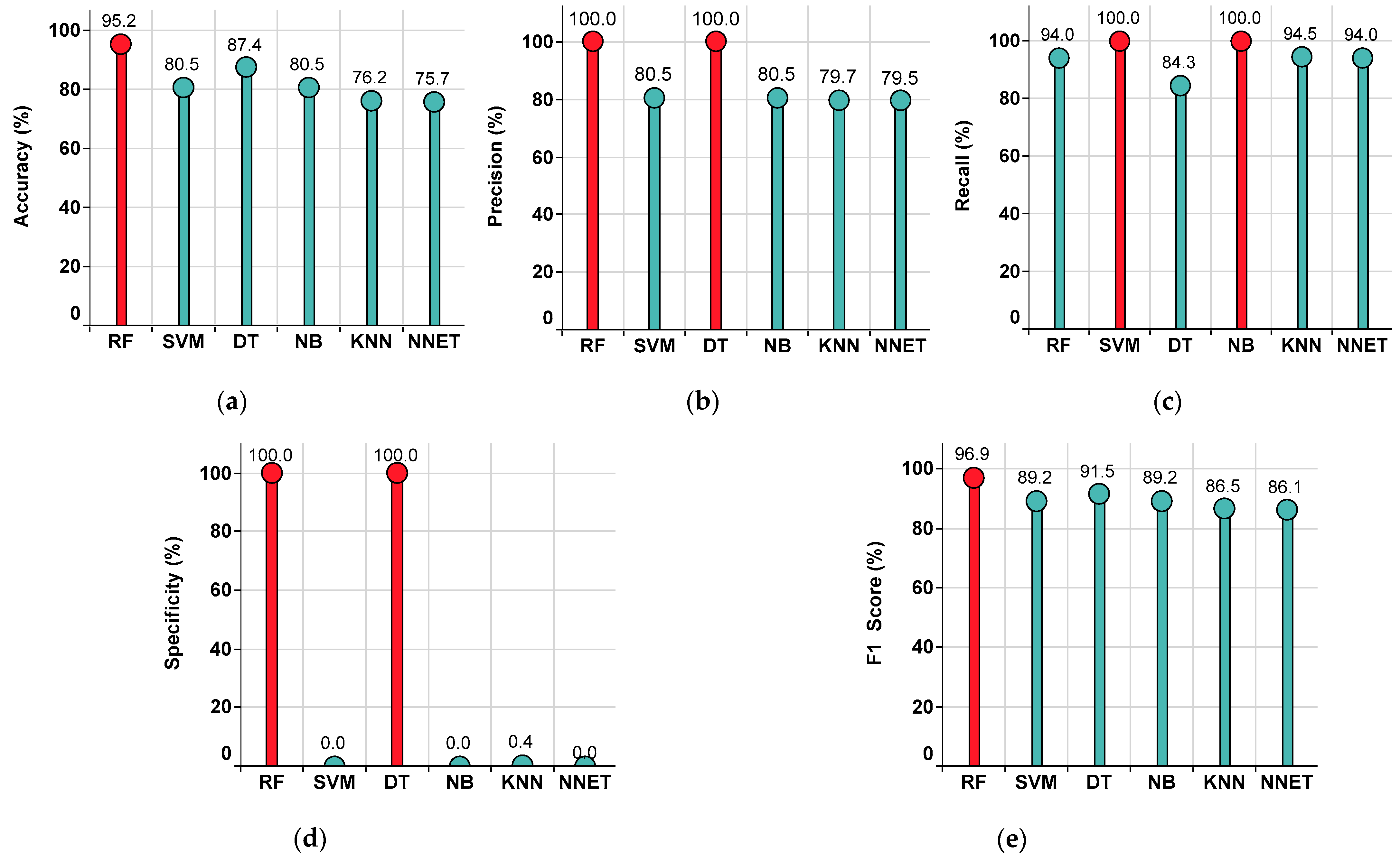
| RF | 95.2 | 100 | 94 | 100 | 96.9 |
| SVM | 80.5 | 80.5 | 100 | 0 | 89.2 |
| DT | 87.4 | 100 | 84.3 | 100 | 91.5 |
| NB | 80.5 | 80.5 | 100 | 0 | 89.2 |
| KNN | 76.2 | 79.7 | 94.5 | 0.4 | 86.5 |
| NNET | 75.7 | 79.5 | 94 | 0 | 86.1 |
| Superior Classifier | RF | RF, DT | SVM, NB | RF, DT | RF |
| Classifier | Accuracy (%) | Precision (%) | Recall (%) | Specificity (%) | F1 Score (%) |
|---|---|---|---|---|---|
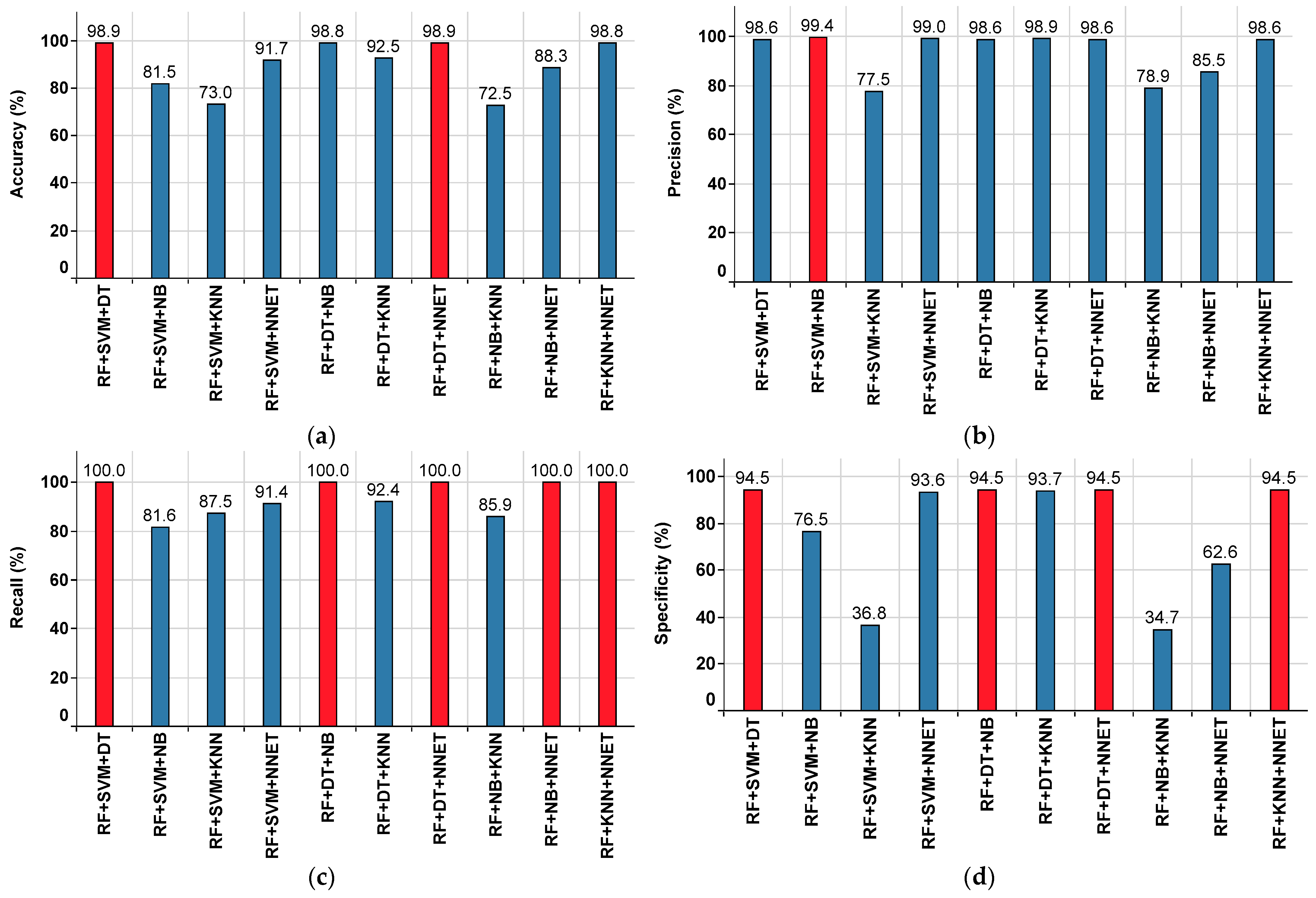
| RF+SVM+DT | 98.9 | 98.6 | 100 | 94.5 | 99.3 |
| RF+SVM+NB | 81.5 | 99.4 | 81.6 | 76.5 | 89.7 |
| RF+SVM+KNN | 73 | 77.5 | 87.5 | 36.8 | 82.2 |
| RF+SVM+NNET | 91.7 | 99 | 91.4 | 93.6 | 95 |
| RF+DT+NB | 98.8 | 98.6 | 100 | 94.5 | 99.3 |
| RF+DT+KNN | 92.5 | 98.9 | 92.4 | 93.7 | 95.5 |
| RF+DT+NNET | 98.9 | 98.6 | 100 | 94.5 | 99.3 |
| RF+NB+KNN | 72.5 | 78.9 | 85.9 | 34.7 | 82.2 |
| RF+NB+NNET | 88.3 | 85.5 | 100 | 62.6 | 92.2 |
| RF+KNN+NNET | 98.8 | 98.6 | 100 | 94.5 | 99.3 |
| Superior Classifier | RF+SVM+DT RF+DT+NNET | RF+SVM+NB | RF+SVM+DT RF+DT+NB RF+DT+NNET RF+NB+NNET RF+KNN+NNET | RF+SVM+DT RF+DT+NB RF+DT+NNET RF+KNN+NNET | RF+SVM+DT RF+DT+NB RF+DT+NNET RF+KNN+NNET |
| Classifier | Accuracy (%) | Precision (%) | Recall (%) | Specificity (%) | F1 Score (%) |
|---|---|---|---|---|---|
| RF+SVM+DT | 78.8 | 97.2 | 80.5 | 19.7 | 88.1 |
| RF+SVM+NB | 75.7 | 88.9 | 82.4 | 31.7 | 85.5 |
| RF+SVM+KNN | 70.9 | 82.9 | 81.4 | 23.3 | 82.1 |
| RF+SVM+NNET | 72.8 | 87.5 | 80.5 | 19.2 | 83.8 |
| RF+DT+NB | 79.9 | 97.8 | 81.1 | 40.1 | 88.7 |
| RF+DT+KNN | 80.2 | 99.3 | 80.6 | 29.5 | 89 |
| RF+DT+NNET | 79.7 | 95.4 | 82.2 | 43.6 | 88.3 |
| RF+NB+KNN | 76.1 | 91.3 | 81.3 | 27 | 86 |
| RF+NB+NNET | 71.1 | 81.3 | 82.6 | 27.4 | 81.9 |
| RF+KNN+NNET | 77.5 | 93.1 | 81.5 | 31.2 | 86.9 |
| Superior Classifier | RF+DT+KNN | RF+DT+KNN | RF+NB+NNET | RF+DT+NNET | RF+DT+KNN |
| Classifier | Accuracy (%) | Precision (%) | Recall (%) | Specificity (%) | F1 Score (%) |
|---|---|---|---|---|---|
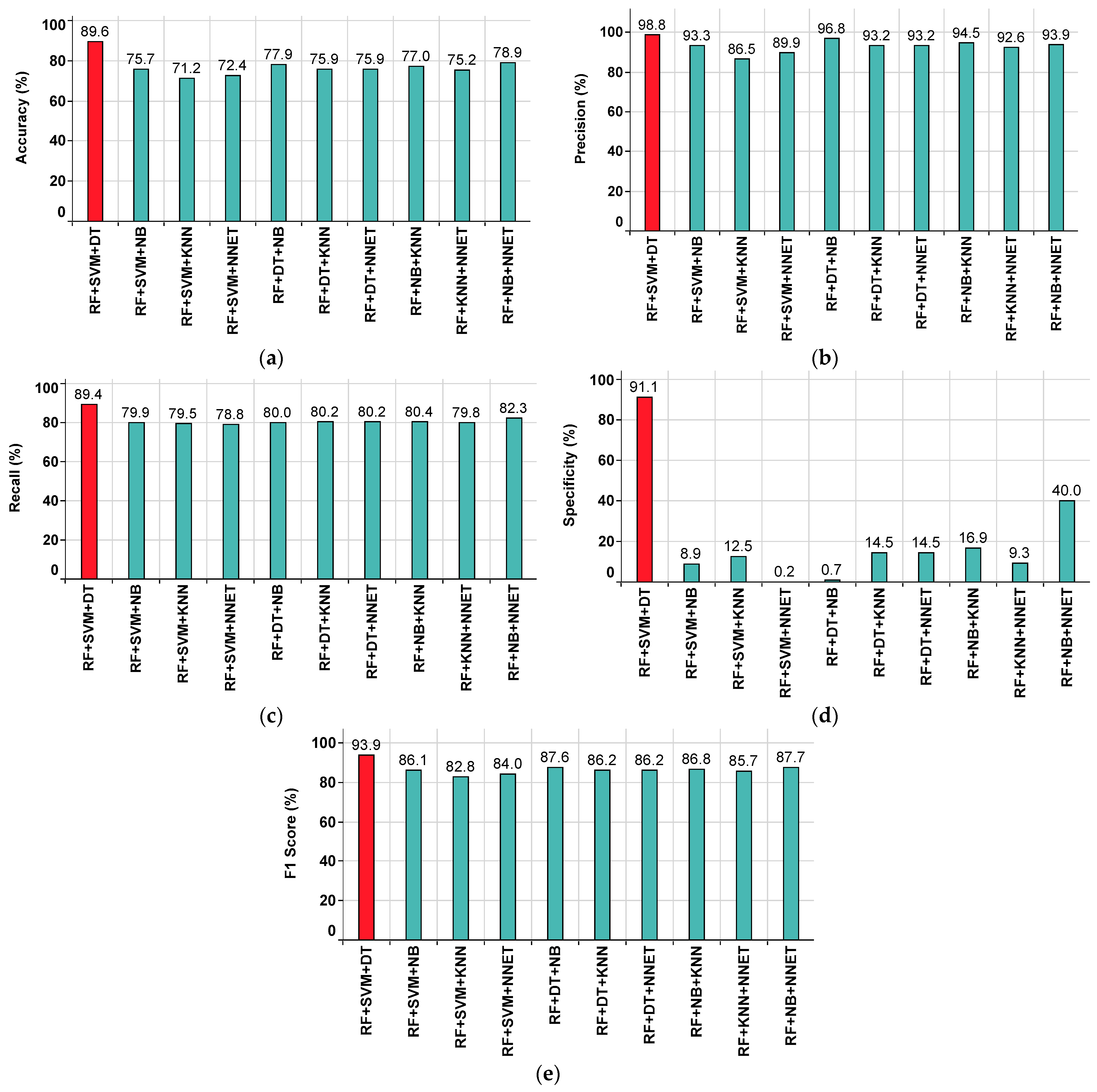
| RF+SVM+DT | 89.6 | 98.8 | 89.4 | 91.1 | 93.9 |
| RF+SVM+NB | 75.7 | 93.3 | 79.9 | 8.9 | 86.1 |
| RF+SVM+KNN | 71.2 | 86.5 | 79.5 | 12.5 | 82.8 |
| RF+SVM+NNET | 72.4 | 89.9 | 78.8 | 0.2 | 84 |
| RF+DT+NB | 77.9 | 96.8 | 80 | 0.7 | 87.6 |
| RF+DT+KNN | 75.9 | 93.2 | 80.2 | 14.5 | 86.2 |
| RF+DT+NNET | 75.9 | 93.2 | 80.2 | 14.5 | 86.2 |
| RF+NB+KNN | 77 | 94.5 | 80.4 | 16.9 | 86.8 |
| RF+NB+NNET | 78.9 | 93.9 | 82.3 | 40 | 87.7 |
| RF+KNN+NNET | 75.2 | 92.6 | 79.8 | 9.3 | 85.7 |
| Superior Classifier | RF+SVM+DT | RF+SVM+DT | RF+SVM+DT | RF+SVM+DT | RF+SVM+DT |
Publisher’s Note: MDPI stays neutral with regard to jurisdictional claims in published maps and institutional affiliations. |
© 2022 by the authors. Licensee MDPI, Basel, Switzerland. This article is an open access article distributed under the terms and conditions of the Creative Commons Attribution (CC BY) license (https://creativecommons.org/licenses/by/4.0/).
Share and Cite
Kasaraneni, P.P.; Venkata Pavan Kumar, Y.; Moganti, G.L.K.; Kannan, R. Machine Learning-Based Ensemble Classifiers for Anomaly Handling in Smart Home Energy Consumption Data. Sensors 2022, 22, 9323. https://doi.org/10.3390/s22239323
Kasaraneni PP, Venkata Pavan Kumar Y, Moganti GLK, Kannan R. Machine Learning-Based Ensemble Classifiers for Anomaly Handling in Smart Home Energy Consumption Data. Sensors. 2022; 22(23):9323. https://doi.org/10.3390/s22239323
Chicago/Turabian StyleKasaraneni, Purna Prakash, Yellapragada Venkata Pavan Kumar, Ganesh Lakshmana Kumar Moganti, and Ramani Kannan. 2022. "Machine Learning-Based Ensemble Classifiers for Anomaly Handling in Smart Home Energy Consumption Data" Sensors 22, no. 23: 9323. https://doi.org/10.3390/s22239323
APA StyleKasaraneni, P. P., Venkata Pavan Kumar, Y., Moganti, G. L. K., & Kannan, R. (2022). Machine Learning-Based Ensemble Classifiers for Anomaly Handling in Smart Home Energy Consumption Data. Sensors, 22(23), 9323. https://doi.org/10.3390/s22239323