
Continuous Monitoring of Suspended Particulate Matter in Tropical Inland Waters by High-Frequency, Above-Water Radiometry
 ,
,  , ,
, ,
Abstract
:1. Introduction
2. Materials and Methods
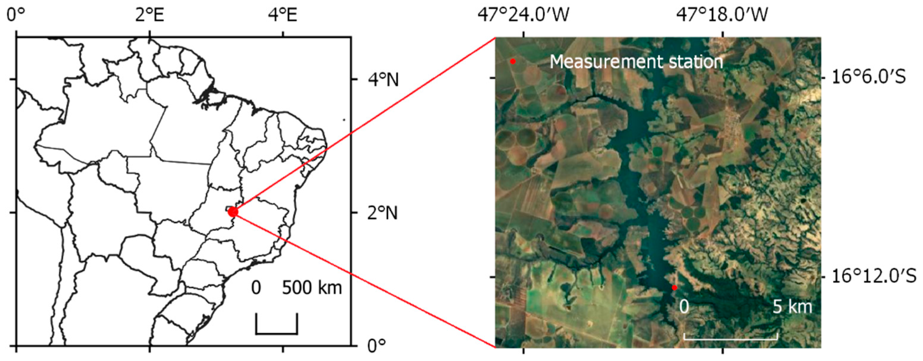
2.1. Test Site
2.2. Radiometric Measurements
2.3. Data Processing
2.3.1. Rrs Calculation Methods
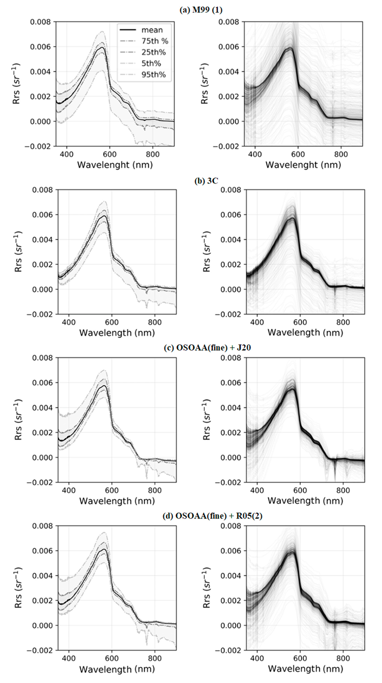
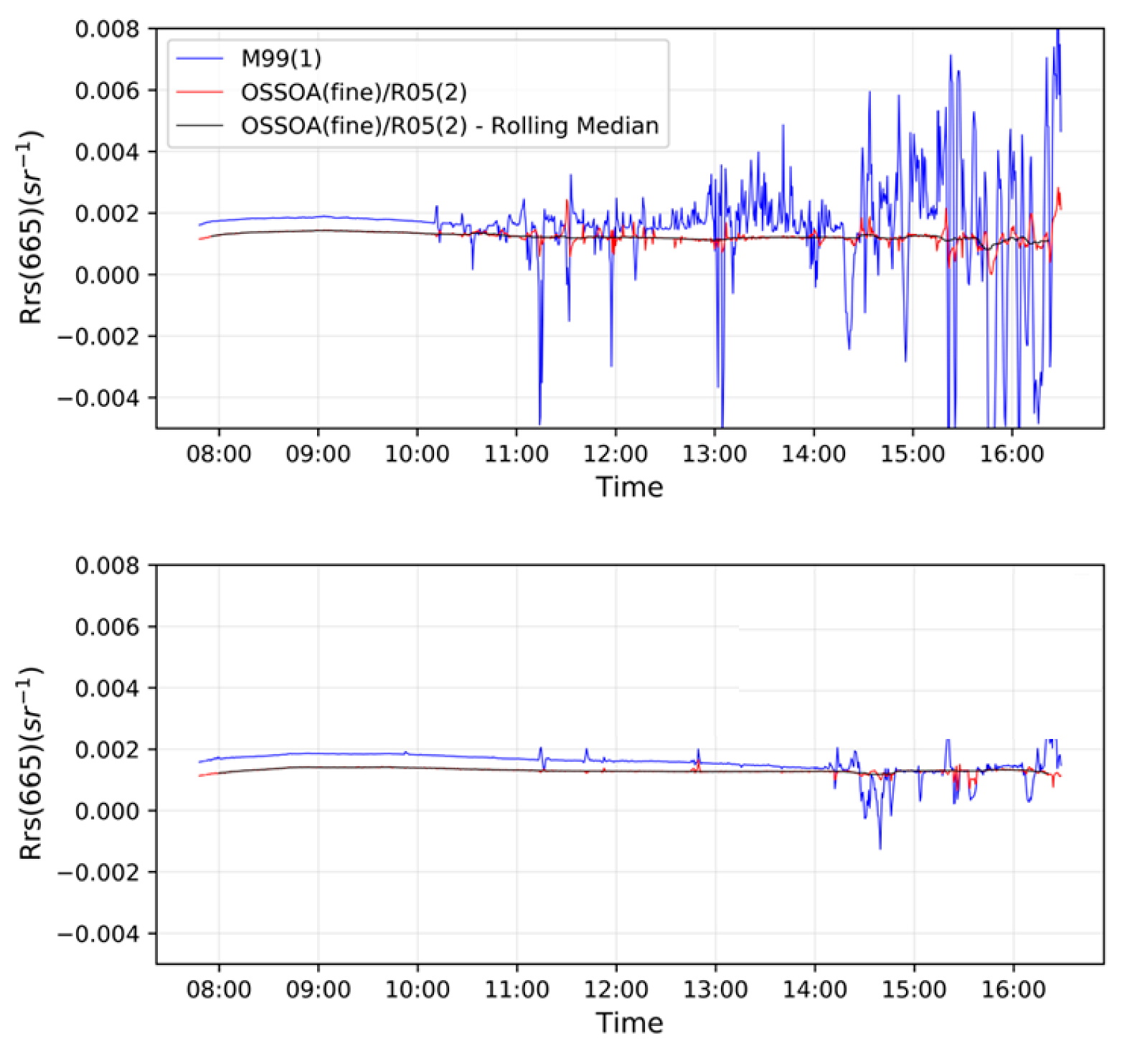
- A value of ρ equal to 0.028 was assessed from the optical modeling for ideal conditions (i.e., perfectly plane surface) and for a viewing angle of 40° and relative azimuth of 135°. This method is henceforth referred to as M99(1) and stands as the simplest correction approach as it does not vary as a function of viewing geometry nor wavelength.
- Rrs calculated using the ρ table from Mobley [28] and applied to Equation (1). The table offers specific ρ-values for combinations of wind speed, relative azimuth, and viewing angle. As such, to find ρ, relative azimuth values were determined at each measurement step, the viewing angle was 40°, and the wind speed was assumed to be 2 m/s for all data points. It should be noted that even though some meteorological wind data were available, it was not accurate enough to be used for shorter time scales; thus, an overall wind velocity average was preferred. Henceforth, it is referred to as M99(2).
- Rrs calculated similarly to M99(2), but using the updated rho table published in [31]. Henceforth, it is referred to as M15.
- Following the abovementioned approach, the ρ-factor was also computed using the radiative transfer code OSOAA [37]. Those computations enable us to directly handle the impact of the light polarization at play in the skylight reflection on the rough water surface [38]. Spectral ρ-factor values were computed for two aerosol-load cases: (i) a fine-mode aerosol model with a modal radius of 0.06 µm and (ii) a coarse aerosol mode with a modal radius of 0.6 µm. For both cases, simulations were performed for a series of aerosol optical thicknesses (from 0 to 1 at 550 nm), several wind speeds (0 to 12 m/s), and for a great number of viewing geometries corresponding to the sun zenith from 0 to 88° (increment 4°) and azimuth angles from 0 to 360° (increment 5°). Note that only clear-sky conditions were considered in those computations. In the rest of the article, the methods using the fine- or the coarse-mode aerosol are referred to as OSOAA(fine) and OSOAA(coarse), respectively.
- The three-component method (hereafter referred to as 3C) exploits an approach in which the spectral dependence of the glint contribution is obtained by distinguishing three irradiance components: the direct solar irradiance, the diffuse molecular-scattered irradiance, and the diffuse aerosol-scattered irradiance. The 3C method combines an aquatic component, in which a semi-analytical, bio-optical model is used to estimate Rrs based on certain optical properties as well as boundary conditions and an atmospheric correction model. An optimization procedure is then used to minimize an objective function related to the differences observed between the modeled and measured values of Lw/Ed, which returns the values of the nine free parameters used in the aquatic and atmospheric models. Rrs is then determined by utilizing the four atmospheric free parameters to calculate a spectrally dependent glint offset and then find Rrs based on measured values of Ed, Lu, and Ld. A more complete description of the model can be seen in the original work [39] as well as in the follow-up paper [40]. It should be noted that, although the 3C method is an Rrs calculation method in the sense that it takes radiometric data as input and outputs Rrs curves, it is also a postprocessing algorithm in the sense used in this article, as it was developed with the intent to correct spectra obtained in suboptimal conditions. For this reason, further postprocessing steps (see next section) used in the present study were not applied to the 3C model.
2.3.2. Rrs Postprocessing Methods
- 1.
- The similarity spectrum, as described in Ruddick et al. [33]. In this method, we assume that the true Rrs is related to the measured Rrs by a flat error factor , as shown in Equation (2).This error factor can be estimated as:in which and are two suitably chosen NIR wavelenghts, and is a related tabulated value provided by the authors. The authors suggest using two suitable pairs of wavelengths, (λ1, λ2) = (720 nm, 780 nm) and (780 nm, 870 nm), which are calculated with = 2.35 and = 1.91, respectively. Both pairs of wavelengths were tested in this study and are further referred to as R05(1) and R05(2).
- 2.
- The correction method proposed by [34]—further referred to as J20, which utilizes the relative height of the water absorption dip-induced reflectance peak at 810 nm—uses RHW as a baseline index. RHW can be calculated using Equations (4) and (5).
- 3.
- An adaptation of the method proposed by [32], in which we fit a power function of the Rrs values between the spectral ranges of 350–380 nm and 890–900 nm, and then subtract the values of the obtained power function from the original Rrs. In the original work, the authors perform the correction directly on the reflectance values (Lu/Ed). Here, we apply the correction scheme to previously calculated Rrs, as presented in the previous section. Henceforth, it is referred to as K13.
2.3.3. Rrs Time-Series Smoothing
2.4. Validation
2.5. SPM Assessment
3. Results
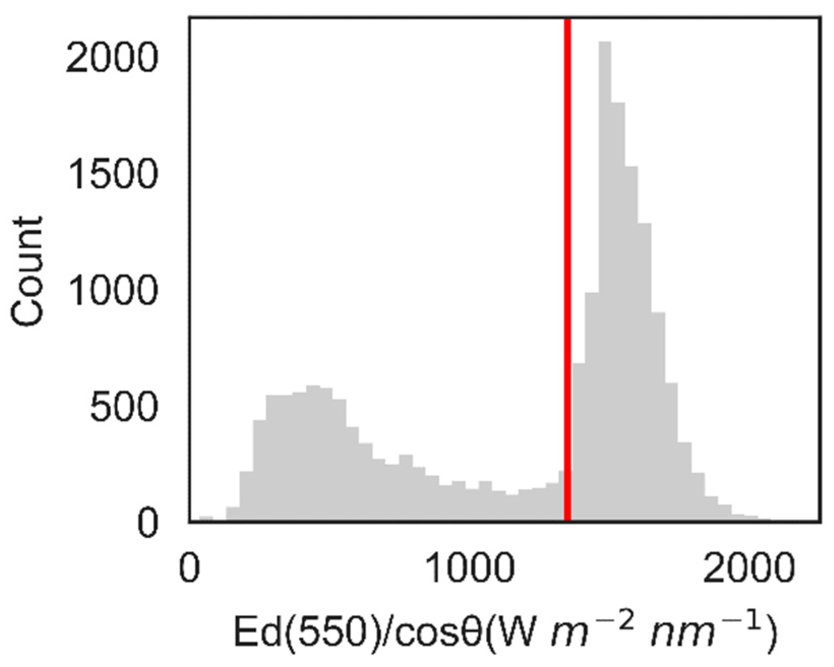
3.1. Radiometric Data
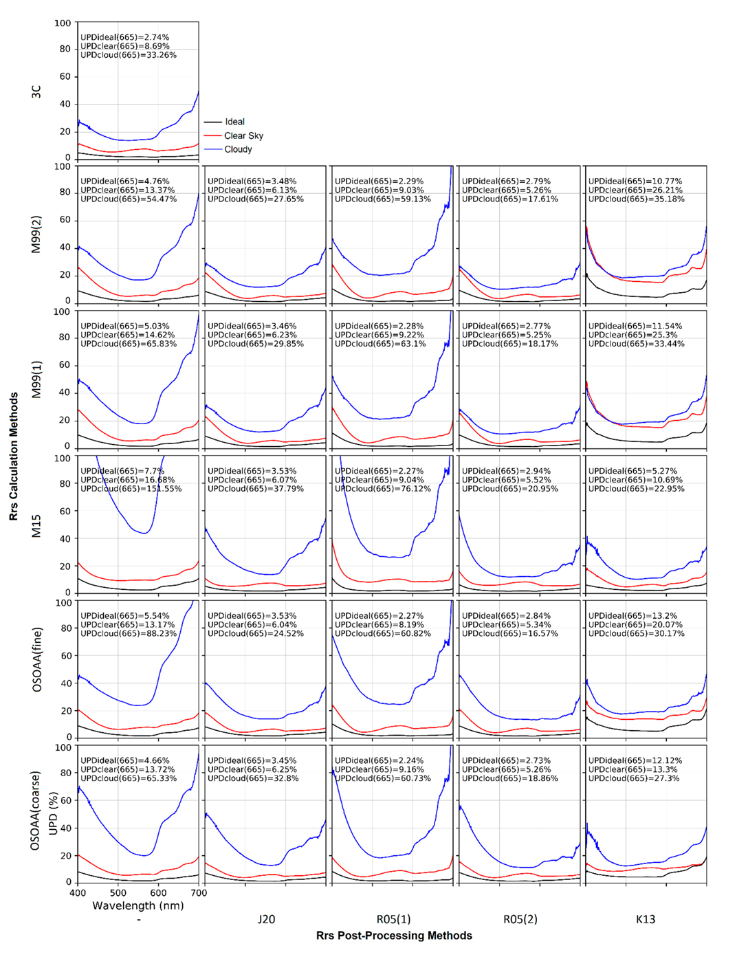
3.2. Obtaining and Processing Remote-Sensing Reflectance
3.3. Time-Series Smoothing
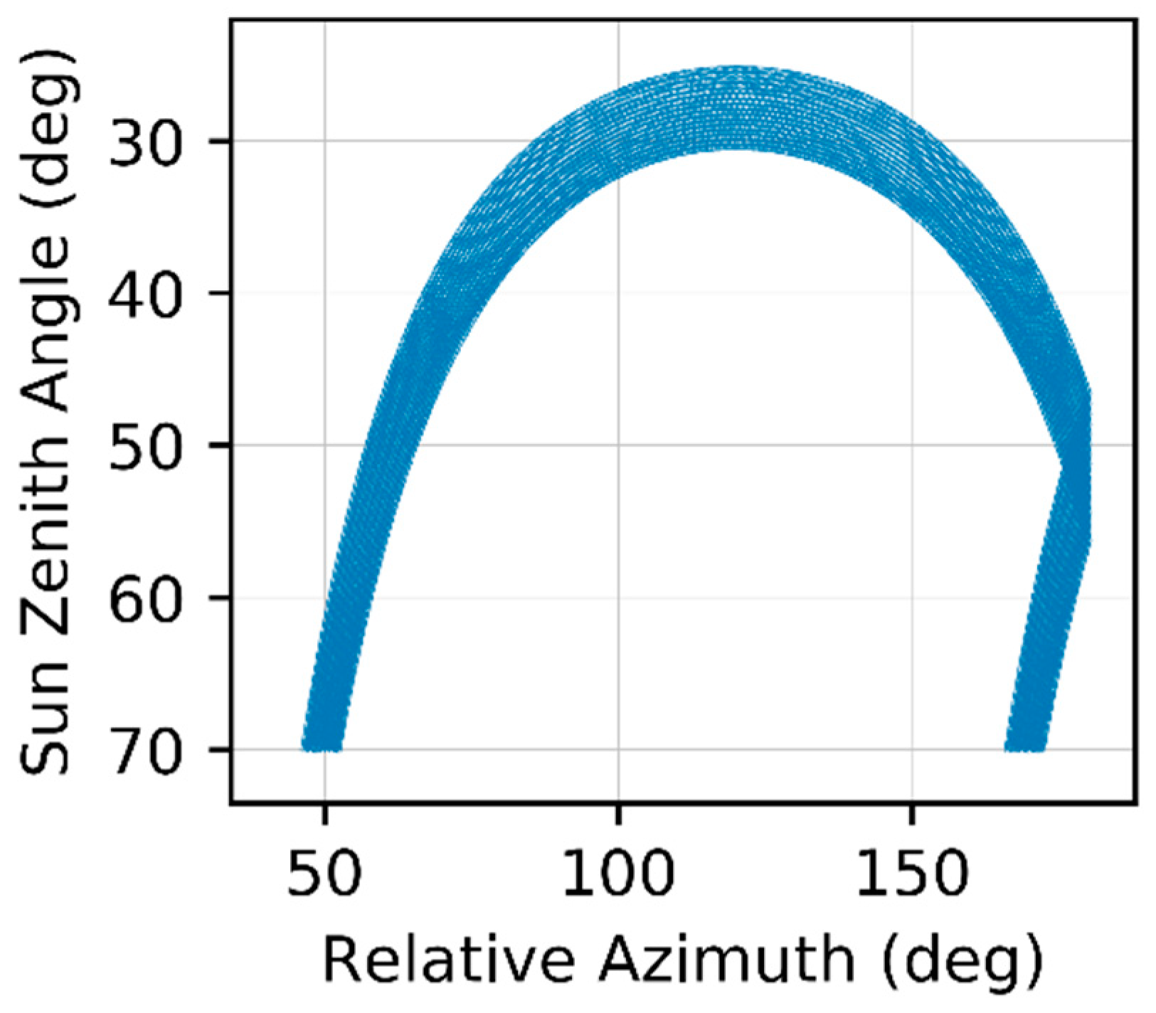
3.4. Variation Due to Sun Angular Position
3.5. SPM Estimation
4. Discussion
Author Contributions
Funding
Institutional Review Board Statement
Informed Consent Statement
Data Availability Statement
Acknowledgments
Conflicts of Interest
References
- Vercruysse, K.; Grabowski, R.C.; Rickson, R.J. Suspended Sediment Transport Dynamics in Rivers: Multi-Scale Drivers of Temporal Variation. Earth-Sci. Rev. 2017, 166, 38–52. [Google Scholar] [CrossRef] [Green Version]
- Gonzalez-Hidalgo, J.C.; Batalla, R.J.; Cerda, A. Catchment Size and Contribution of the Largest Daily Events to Suspended Sediment Load on a Continental Scale. Catena 2013, 102, 40–45. [Google Scholar] [CrossRef]
- Mano, V.; Nemery, J.; Belleudy, P.; Poirel, A. Assessment of Suspended Sediment Transport in Four Alpine Watersheds (France): Influence of the Climatic Regime. Hydrol. Process. 2009, 23, 777–792. [Google Scholar] [CrossRef]
- Hauer, C.; Leitner, P.; Unfer, G.; Pulg, U.; Habersack, H.; Graf, W. The Role of Sediment and Sediment Dynamics in the Aquatic Environment. In Riverine Ecosystem Management; Springer: Cham, Switzerland, 2018; pp. 151–169. [Google Scholar]
- Basson, G. Sedimentation and Sustainable Use of Reservoirs and River Systems; International Commission on Large Dams (ICOLD) Bulletin; CRC Press: Boca Raton, FL, USA, 2010. [Google Scholar]
- Hauer, C.; Holzapfel, P.; Flödl, P.; Wagner, B.; Graf, W.; Leitner, P.; Haimann, M.; Holzer, G.; Haun, S.; Habersack, H.; et al. Controlled Reservoir Drawdown-Challenges for Sediment Management and Integrative Monitoring: An Austrian Case Study-Part B: Local Scale. Water 2020, 12, 1058. [Google Scholar] [CrossRef] [Green Version]
- Wang, X.; Yang, W. Water Quality Monitoring and Evaluation Using Remote-Sensing Techniques in China: A Systematic Review. Ecosyst. Health Sustain. 2019, 5, 47–56. [Google Scholar] [CrossRef] [Green Version]
- Topp, S.N.; Pavelsky, T.M.; Jensen, D.; Simard, M.; Ross, M.R.V. Research Trends in the Use of Remote Sensing for Inland Water Quality Science: Moving towards Multidisciplinary Applications. Water 2020, 12, 169. [Google Scholar] [CrossRef] [Green Version]
- Sagan, V.; Peterson, K.T.; Maimaitijiang, M.; Sidike, P.; Sloan, J.; Greeling, B.A.; Maalouf, S.; Adams, C. Monitoring Inland Water Quality Using Remote Sensing: Potential and Limitations of Spectral Indices, Bio-Optical Simulations, Machine Learning, and Cloud Computing. Earth-Sci. Rev. 2020, 205, 103187. [Google Scholar] [CrossRef]
- Yang, H.; Kong, J.; Hu, H.; Du, Y.; Gao, M.; Chen, F. A Review of Remote Sensing for Water Quality Retrieval: Progress and Challenges. Remote Sens. 2022, 14, 1770. [Google Scholar] [CrossRef]
- Novoa, S.; Doxaran, D.; Ody, A.; Vanhellemont, Q.; Lafon, V.; Lubac, B.; Gernez, P. Atmospheric Corrections and Multi-Conditional Algorithm for Multi-Sensor Remote Sensing of Suspended Particulate Matter in Low-to-High Turbidity Levels Coastal Waters. Remote Sens. 2017, 9, 61. [Google Scholar] [CrossRef] [Green Version]
- de Oliveira Fagundes, H.; Cauduro Dias de Paiva, R.; Mainardi Fan, F.; Costa Buarque, D.; César Fassoni-Andrade, A. Sediment Modeling of a Large-Scale Basin Supported by Remote Sensing and in-Situ Observations. Catena 2020, 190, 104535. [Google Scholar] [CrossRef]
- Wang, C.; Li, W.; Chen, S.; Li, D.; Wang, D.; Liu, J. The Spatial and Temporal Variation of Total Suspended Solid Concentration in Pearl River Estuary during 1987–2015 Based on Remote Sensing. Sci. Total Environ. 2018, 618, 1125–1138. [Google Scholar] [CrossRef] [PubMed]
- Espinoza-Villar, R.; Martinez, J.M.; Armijos, E.; Espinoza, J.C.; Filizola, N.; Dos Santos, A.; Willems, B.; Fraizy, P.; Santini, W.; Vauchel, P. Spatio-Temporal Monitoring of Suspended Sediments in the Solimões River (2000–2014). Comptes Rendus Geosci. 2018, 350, 4–12. [Google Scholar] [CrossRef]
- Olivetti, D.; Roig, H.; Martinez, J.M.; Borges, H.; Ferreira, A.; Casari, R.; Salles, L.; Malta, E. Low-Cost Unmanned Aerial Multispectral Imagery for Siltation Monitoring in Reservoirs. Remote Sens. 2020, 12, 1855. [Google Scholar] [CrossRef]
- Sibanda, M.; Mutanga, O.; Chimonyo, V.G.P.; Clulow, A.D.; Shoko, C.; Mazvimavi, D.; Dube, T.; Mabhaudhi, T. Application of Drone Technologies in SurfaceWater Resources Monitoring and Assessment: A Systematic Review of Progress, Challenges, and Opportunities in the Global South. Drones 2021, 5, 84, Erratum in Drones 2022, 6, 84. [Google Scholar] [CrossRef]
- Skarbøvik, E.; Stålnacke, P.; Bogen, J.; Bønsnes, T.E. Impact of Sampling Frequency on Mean Concentrations and Estimated Loads of Suspended Sediment in a Norwegian River: Implications for Water Management. Sci. Total Environ. 2012, 433, 462–471. [Google Scholar] [CrossRef] [PubMed]
- Moatar, F.; Person, G.; Meybeck, M.; Coynel, A.; Etcheber, H.; Crouzet, P. The Influence of Contrasting Suspended Particulate Matter Transport Regimes on the Bias and Precision of Flux Estimates. Sci. Total Environ. 2006, 370, 515–531. [Google Scholar] [CrossRef]
- López-Tarazón, J.A.; Batalla, R.J.; Vericat, D.; Francke, T. Suspended Sediment Transport in a Highly Erodible Catchment: The River Isábena (Southern Pyrenees). Geomorphology 2009, 109, 210–221. [Google Scholar] [CrossRef]
- Navratil, O.; Esteves, M.; Legout, C.; Gratiot, N.; Nemery, J.; Willmore, S.; Grangeon, T. Global Uncertainty Analysis of Suspended Sediment Monitoring Using Turbidimeter in a Small Mountainous River Catchment. J. Hydrol. 2011, 398, 246–259. [Google Scholar] [CrossRef]
- Esteves, M.; Legout, C.; Navratil, O.; Evrard, O. Medium Term High Frequency Observation of Discharges and Suspended Sediment in a Mediterranean Mountainous Catchment. J. Hydrol. 2019, 568, 562–574. [Google Scholar] [CrossRef]
- Fettweis, M.; Riethmüller, R.; Verney, R.; Becker, M.; Backers, J.; Baeye, M.; Chapalain, M.; Claeys, S.; Claus, J.; Cox, T.; et al. Uncertainties Associated with in Situ High-Frequency Long-Term Observations of Suspended Particulate Matter Concentration Using Optical and Acoustic Sensors. Prog. Oceanogr. 2019, 178, 102162. [Google Scholar] [CrossRef]
- Arabi, B.; Salama, M.S.; Wernand, M.R.; Verhoef, W. Remote Sensing of Water Constituent Concentrations Using Time Series of In-Situ Hyperspectral Measurements in the Wadden Sea. Remote Sens. Environ. 2018, 216, 154–170. [Google Scholar] [CrossRef]
- Arabi, B.; Salama, M.S.; Pitarch, J.; Verhoef, W. Integration of In-Situ and Multi-Sensor Satellite Observations for Long-Term Water Quality Monitoring in Coastal Areas. Remote Sens. Environ. 2020, 239, 111632. [Google Scholar] [CrossRef]
- Cao, Q.; Yu, G.; Sun, S.; Dou, Y.; Li, H.; Qiao, Z. Monitoring Water Quality of the Haihe River Based on Ground-Based Hyperspectral Remote Sensing. Water 2022, 14, 22. [Google Scholar] [CrossRef]
- Harmel, T.; Gilerson, A.; Hlaing, S.; Weidemann, A.; Arnone, R.; Ahmed, S. Long Island Sound Coastal Observatory: Assessment of above-Water Radiometric Measurement Uncertainties Using Collocated Multi and Hyper-Spectral Systems: Reply to Comment. Appl. Opt. 2012, 51, 3893. [Google Scholar] [CrossRef]
- Vansteenwegen, D.; Ruddick, K.; Cattrijsse, A.; Vanhellemont, Q.; Beck, M. The Pan-and-Tilt Hyperspectral Radiometer System (PANTHYR) for Autonomous Satellite Validation Measurements-Prototype Design and Testing. Remote Sens. 2019, 11, 1360. [Google Scholar] [CrossRef] [Green Version]
- Mobley, C.D. Estimation of the Remote-Sensing Reflectance from above-Surface Measurements. Appl. Opt. 1999, 38, 7442. [Google Scholar] [CrossRef]
- Ruddick, K.G.; Voss, K.; Boss, E.; Castagna, A.; Frouin, R.; Gilerson, A.; Hieronymi, M.; Carol Johnson, B.; Kuusk, J.; Lee, Z.; et al. A Review of Protocols for Fiducial Reference Measurements of Water-Leaving Radiance for Validation of Satellite Remote-Sensing Data over Water. Remote Sens. 2019, 11, 2198. [Google Scholar] [CrossRef] [Green Version]
- Zibordi, G.; Voss, K.; Johnson, B.C.; Mueller, J.L. Protocols for Satellite Ocean Colour Data Validation: In Situ Optical Radiometry. In Ocean Optics and Biogeochemistry Protocols for Satellite Ocean Colour Sensor Validation; IOCCG Protocol Series; IOCCG: Dartmouth, NS, Canada, 2019; Volume 3, p. 3. [Google Scholar]
- Mobley, C.D. Polarized Reflectance and Transmittance Properties of Windblown Sea Surfaces. Appl. Opt. 2015, 54, 4828–4849. [Google Scholar] [CrossRef]
- Kutser, T.; Vahtmäe, E.; Paavel, B.; Kauer, T. Removing Glint Effects from Field Radiometry Data Measured in Optically Complex Coastal and Inland Waters. Remote Sens. Environ. 2013, 133, 85–89. [Google Scholar] [CrossRef]
- Ruddick, K.; De Cauwer, V.; Van Mol, B. Use of the near Infrared Similarity Reflectance Spectrum for the Quality Control of Remote Sensing Data. Remote Sens. Coast. Ocean. Environ. 2005, 5885, 588501. [Google Scholar] [CrossRef]
- Jiang, D.; Matsushita, B.; Yang, W. A Simple and Effective Method for Removing Residual Reflected Skylight in Above-Water Remote Sensing Reflectance Measurements. ISPRS J. Photogramm. Remote Sens. 2020, 165, 16–27. [Google Scholar] [CrossRef]
- Condé, R.d.C.; Martinez, J.M.; Pessotto, M.A.; Villar, R.; Cochonneau, G.; Henry, R.; Lopes, W.; Nogueira, M. Indirect Assessment of Sedimentation in Hydropower Dams Using MODIS Remote Sensing Images. Remote Sens. 2019, 11, 314. [Google Scholar] [CrossRef] [Green Version]
- Walter, W.G. Standard Methods for the Examination of Water and Wastewater, 11th ed.; American Public Health Association: Washington, DC, USA, 1961; Volume 51, ISBN 0875532357. [Google Scholar]
- Chami, M.; Lafrance, B.; Fougnie, B.; Chowdhary, J.; Harmel, T.; Waquet, F. OSOAA: A Vector Radiative Transfer Model of Coupled Atmosphere-Ocean System for a Rough Sea Surface Application to the Estimates of the Directional Variations of the Water Leaving Reflectance to Better Process Multi-Angular Satellite Sensors Data over the Ocean. Opt. Express 2015, 23, 27829. [Google Scholar] [CrossRef] [Green Version]
- Harmel, T.; Gilerson, A.; Tonizzo, A.; Chowdhary, J.; Weidemann, A.; Arnone, R.; Ahmed, S. Polarization Impacts on the Water-Leaving Radiance Retrieval from above-Water Radiometric Measurements. Appl. Opt. 2012, 51, 8324. [Google Scholar] [CrossRef] [PubMed]
- Groetsch, P.M.M.; Gege, P.; Simis, S.G.H.; Eleveld, M.A.; Peters, S.W.M. Validation of a Spectral Correction Procedure for Sun and Sky Reflections in Above-Water Reflectance Measurements. Opt. Express 2017, 25, A742. [Google Scholar] [CrossRef] [PubMed] [Green Version]
- Pitarch, J.; Talone, M.; Zibordi, G.; Groetsch, P. Determination of the Remote-Sensing Reflectance from above-Water Measurements with the “3C Model”: A Further Assessment. Opt. Express 2020, 28, 15885. [Google Scholar] [CrossRef] [PubMed]
- Nechad, B.; Ruddick, K.G.; Park, Y. Calibration and Validation of a Generic Multisensor Algorithm for Mapping of Total Suspended Matter in Turbid Waters. Remote Sens. Environ. 2010, 114, 854–866. [Google Scholar] [CrossRef]
- Balasubramanian, S.V.; Pahlevan, N.; Smith, B.; Binding, C.; Schalles, J.; Loisel, H.; Gurlin, D.; Greb, S.; Alikas, K.; Randla, M.; et al. Robust Algorithm for Estimating Total Suspended Solids (TSS) in Inland and Nearshore Coastal Waters. Remote Sens. Environ. 2020, 246, 111768. [Google Scholar] [CrossRef]
- Lee, Z.; Carder, K.L.; Arnone, R.A. Deriving Inherent Optical Properties from Water Color: A Multiband Quasi-Analytical Algorithm for Optically Deep Waters. Appl. Opt. 2002, 41, 5755. [Google Scholar] [CrossRef]
- Dethier, E.N.; Renshaw, C.E.; Magilligan, F.J. Toward Improved Accuracy of Remote Sensing Approaches for Quantifying Suspended Sediment: Implications for Suspended-Sediment Monitoring. J. Geophys. Res. Earth Surf. 2020, 125, e2019JF005033. [Google Scholar] [CrossRef]
- Volpe, V.; Silvestri, S.; Marani, M. Remote Sensing Retrieval of Suspended Sediment Concentration in Shallow Waters. Remote Sens. Environ. 2011, 115, 44–54. [Google Scholar] [CrossRef]
- Marinho, R.R.; Harmel, T.; Martinez, J.M.; Junior, N.P.F. Spatiotemporal Dynamics of Suspended Sediments in the Negro River, Amazon Basin, from in Situ and Sentinel-2 Remote Sensing Data. ISPRS Int. J. Geo-Inf. 2021, 10, 86. [Google Scholar] [CrossRef]
- Dang, T.D.; Cochrane, T.A.; Arias, M.E. Quantifying Suspended Sediment Dynamics in Mega Deltas Using Remote Sensing Data: A Case Study of the Mekong Floodplains. Int. J. Appl. Earth Obs. Geo-Inf. 2018, 68, 105–115. [Google Scholar] [CrossRef]
- Umar, M.; Rhoads, B.L.; Greenberg, J.A. Use of Multispectral Satellite Remote Sensing to Assess Mixing of Suspended Sediment Downstream of Large River Confluences. J. Hydrol. 2018, 556, 325–338. [Google Scholar] [CrossRef]


| CV at 400 nm | CV at 550 nm | CV at 665 nm | |
|---|---|---|---|
| Lu/cos(θ) | 29.7% | 37.6% | 60.2% |
| Ld/cos(θ) | 48.2% | 86.2% | 108.7% |
| Ed/cos(θ) | 41.2% | 45.5% | 48.0% |
| No Smoothing | With Smoothing | ||||
|---|---|---|---|---|---|
| Rrs Model | SPM Model | Mean (g/m3) | CV (%) | Mean (g/m3) | CV (%) |
| M99(1) | N10 | 1.74 | 69.5% | 1.68 | 53.6% |
| SOLID | 2.23 | 17.5% | 2.24 | 10.3% | |
| 3C | N10 | 1.76 | 43.8% | 1.72 | 25.6% |
| SOLID | 2.24 | 10.7% | 2.26 | 4.9% | |
| OSOAA(fine) J20 | N10 | 1.60 | 52.5% | 1.58 | 30.4% |
| SOLID | 2.32 | 7.3% | 2.33 | 3.9% | |
| OSOAA(fine) R05(2) | N10 | 1.65 | 48.5% | 1.63 | 29.4% |
| SOLID | 2.20 | 4.1% | 2.2 | 2.7% | |
Publisher’s Note: MDPI stays neutral with regard to jurisdictional claims in published maps and institutional affiliations. |
© 2022 by the authors. Licensee MDPI, Basel, Switzerland. This article is an open access article distributed under the terms and conditions of the Creative Commons Attribution (CC BY) license (https://creativecommons.org/licenses/by/4.0/).
Share and Cite
Borges, H.D.; Martinez, J.-M.; Harmel, T.; Cicerelli, R.E.; Olivetti, D.; Roig, H.L. Continuous Monitoring of Suspended Particulate Matter in Tropical Inland Waters by High-Frequency, Above-Water Radiometry. Sensors 2022, 22, 8731. https://doi.org/10.3390/s22228731
Borges HD, Martinez J-M, Harmel T, Cicerelli RE, Olivetti D, Roig HL. Continuous Monitoring of Suspended Particulate Matter in Tropical Inland Waters by High-Frequency, Above-Water Radiometry. Sensors. 2022; 22(22):8731. https://doi.org/10.3390/s22228731
Chicago/Turabian StyleBorges, Henrique Dantas, Jean-Michel Martinez, Tristan Harmel, Rejane Ennes Cicerelli, Diogo Olivetti, and Henrique Llacer Roig. 2022. "Continuous Monitoring of Suspended Particulate Matter in Tropical Inland Waters by High-Frequency, Above-Water Radiometry" Sensors 22, no. 22: 8731. https://doi.org/10.3390/s22228731
APA StyleBorges, H. D., Martinez, J.-M., Harmel, T., Cicerelli, R. E., Olivetti, D., & Roig, H. L. (2022). Continuous Monitoring of Suspended Particulate Matter in Tropical Inland Waters by High-Frequency, Above-Water Radiometry. Sensors, 22(22), 8731. https://doi.org/10.3390/s22228731