Abstract
This paper presents an experimental validation of deep learning-based direction-of-arrival (DoA) estimation by using realistic data collected via universal software radio peripheral (USRP). Deep neural network (DNN) and convolutional neural network (CNN) structures are designed to estimate the DoA. Two types of data are used for training networks. One is the data synthesized by the signal model, and the other is the data collected by USRP. Here, the signal model considers both mutual coupling and multipath signals. Experimental results show that the estimation performance is most accurate when training DNN and CNN with the collected data. Furthermore, the estimation tends to be poor in the indoor environment, which suffers from the strong non-line-of-sight (NLoS) signals.
1. Introduction
Direction-of-arrival (DoA) estimation is one of the long-studied research topics in array signal processing. DoA estimation algorithms have been adopted in various applications, such as localization and radar [1]. Traditional DoA estimation algorithms such as MUSIC [2] and ESPRIT [3] are proposed based on the characteristic of the signal model. Although they can ideally achieve high estimation accuracy and resolution, unexpected problems (e.g., multipath effect [4], gain-phase error [5], mutual coupling [6], antenna misalignment [7], etc.) may exist in practice. In this case, the signal model cannot capture the characteristics of a real received signal, thereby causing degradation of the DoA estimation performance.
There have been various studies to deal with problems that may cause model mismatch. One of these studies is coherent DoA estimation, which can estimate multipath signals impinging from different directions [4,8,9]. On the other hand, there are problems induced by hardware impairments such as gain-phase error, mutual coupling, and antenna misalignment. There have been efforts to calibrate these errors without using reference signals, where [5,10,11] deal with gain-phase error, [6,12,13] deal with mutual coupling between antennas in an array, and [7,14] deal with the errors in the steering vector that can be caused by antenna misalignment. However, the performance of the aforementioned works may degrade when several problems simultaneously occur or there are more unexpected problems.
After the introduction of deep learning [15], DoA estimation algorithms based on various types of neural network (NN) have been proposed in [16,17,18,19,20]. One of the benefits of using deep learning is that the user does not have to know the exact signal model if there are sufficient training data. For this reason, it is expected that the deep learning-based DoA estimation does not suffer from model mismatch problems by using data that capture all kinds of errors (e.g., actual measured data). In [16,17], deep neural network (DNN)-based DoA estimation was proposed, where these works report that the DNN-based estimation is more accurate than the traditional DoA estimation. After the proposal of the DNN-based DoA estimation, convolutional neural network (CNN)-based DoA estimation has been studied in [18,19]. The CNN-based DoA estimation shows better estimation accuracy and resolution compared to the DNN-based DoA estimation. In [20], the DoA estimation based on unsupervised learning was proposed, where unsupervised learning can make data collection easier since data labeling is not required. In recent works, there have been efforts to exploit features of classical DoA estimation, rather than solely depending on NN. Refs. [21,22,23] respectively employ DNN, CNN, and recurrent neural network (RNN) to estimate the ideal noiseless covariance matrix, which is denoted as a pseudo covariance matrix. Then, the classical DoA estimation such as MUSIC and root-MUSIC estimates the DoA with pseudo covariance matrix. In [24], the residual neural network (ResNet) first estimates the candidates of DoAs. From the candidates, the classical maximum likelihood estimation (MLE) [25] picks the final DoAs. A combination of these two methods enhances the accuracy while achieving lower complexity than only using MLE.
However, the existing works on the deep learning-based DoA estimation lack experimental validation, even though the deep learning-based DoA estimation is expected to be effective in a practical situation where there are many problems that cause a model mismatch. In this paper, we validate deep learning-based DoA estimation with realistic data collected by a universal software radio peripheral (USRP). In the experiment, two types of data—data synthesized by the signal model and data collected by USRP—are used for training networks. The estimation accuracy is then analyzed according to the type of training data.
2. System Model
In this paper, we consider one transmitter, which is equipped with an omni-directional antenna. A receiver is equipped with a uniform linear array (ULA), which has M antenna elements. The spacing between adjacent antennas is set to half-wavelength , where denotes the wavelength of the transmitted signal.
To generate the data for training DNN and CNN, the signal model should be defined. Here, the generated data are expected to be well-suited for training if the signal model can capture the state of the hardware systems. Among the many kinds of hardware-induced problems, the gain-phase error in our systems is calibrated using the method in [26]. The antenna spacing is designed to be half-wavelength so that there is no antenna misalignment. However, the current systems cannot calibrate mutual coupling and multipath effects. Thus, in this paper, we consider mutual coupling and multipath effects to design the received signal model.
An array manifold vector whose DoA is , can be given as follows:
To capture mutual coupling and multipath effects, we model a received signal as:
where denotes the mutual coupling matrix [27]. P denotes the number of non-line-of-sight (NLoS) paths. and respectively denote the channel gain and the DoA of the p-th signal path. Specifically, and denote the channel gain and the DoA of the line-of-sight (LoS) path. denotes a signal vector, whose power equals . D is a number of signal snapshots. is a noise matrix, whose entries all follow . denotes the power of the noise. , the covariance matrix of , can be defined as:
3. Deep Learning Network Structure for DoA Estimation
This section introduces two network structures for DoA estimation, which are respectively based on DNN and CNN. A scheme of deep learning-based DoA estimation is depicted in Figure 1. In the presence of multipath signals and mutual couplings, the deep learning network aims to estimate the DoA of the LoS path using the covariance matrix.
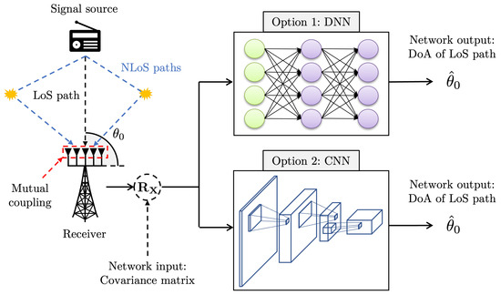
Figure 1.
A scheme of deep learning-based DoA estimation. The proposed DNN or CNN structure estimates the DoA of the LoS path in the presence of multipath signals and mutual coupling.
3.1. DoA Estimation via Deep Neural Network
Since the input of the DNN has to be a real vector, the input of the DNN is formulated as:
where denotes the vectorization. and respectively denote the real and imaginary values of the argument. denotes the Frobenius norm.
Letting L, , and respectively denote the number of dense layers, the output of the l-th layer, and the size of , can be given by:
where . denotes the ReLU function, which is widely used as the activation function of the neuron [15]. and denote the weights and the bias of the l-th layers. The loss function of the DNN is given by MSE, , where denotes the estimated value of the DoA of the LoS path. The weights and the bias that minimize the loss function can be denoted as:
where and denote the weights and the bias of the l-th dense layer that minimize the loss function. (6) is implemented by back propagation. A parameter setting for the DNN structure used in this paper is summarized in Table 1.

Table 1.
Parameter setting for DNN structure.
3.2. DoA Estimation via Convolutional Neural Network
Since the input of the CNN can be a three-dimensional matrix, the input of the CNN is formulated as:
where ; denotes an operator that overlaps matrices with the same dimension.
An output of the k-th convolutional layer, , can be represented as in [18]:
where ∗ denotes the convolution. denotes the j-th channel of 3D tensor and . and K are the number of kernels and the number of convolutional layers. denotes the j-th kernel in the k-th layer, where is a dimension of the kernels in the k-th layer. denotes the bias for the j-th kernel in the k-th convolutional layer.
After undergoing K convolutional layers, all values of are summed to yield the output. The loss function of the CNN is given by MSE, . The convolution kernel and the bias that minimize the loss function can be given by:
where and denote the j-th convolution kernel and the bias of the k-th layer that minimize the loss function. (9) is implemented by back propagation. A parameter setting for CNN structure used in this paper is summarized in Table 2.

Table 2.
Parameter setting for CNN structure.
4. Experimental Results and Discussion
4.1. Experimental Setup
In this paper, we use two types of data. One is synthesized data generated based on the signal model in (2). We generated 4,000,000 synthesized data via MATLAB. Here, M, D, and the maximum mutual coupling strength were respectively set to 4, 512, and . was fixed to 1. P was randomly set between 0 and 10, and was randomly set between 0 and . The signal-to-noise ratio (SNR) of synthesized data was also randomly set between 0 dB and 20 dB, where the SNR is defined as [dB].
Another type of data is that collected with USRP. Note that this data may differ from the signal model in (2). If so, the estimation is expected to be inaccurate when the network is trained with synthesized data. Figure 2 shows a transmitter and a receiver used for the experiment. The transmitter mainly consists of USRP 2954R and the transmitting antenna. The receiver mainly consists of USRP 2955 and a receiving antenna array. Although USRP 2954R and USRP 2955 support a frequency range of 10 MHz–6 GHz, we set the carrier frequency to 5.8 GHz, which is the center frequency of antennas. For this reason, the spacing between patch antennas in the array is designed to the half-wavelength of 5.8 GHz. USRP 2954R generates a 5.8 GHz cosine wave, and the transmitting antenna emits the wave. Then, USRP 2955 receives the cosine wave via the antenna array at a sampling rate of 1 MHz. By using GNU radio, the covariance matrices of the received signals are collected with USRP 2955.
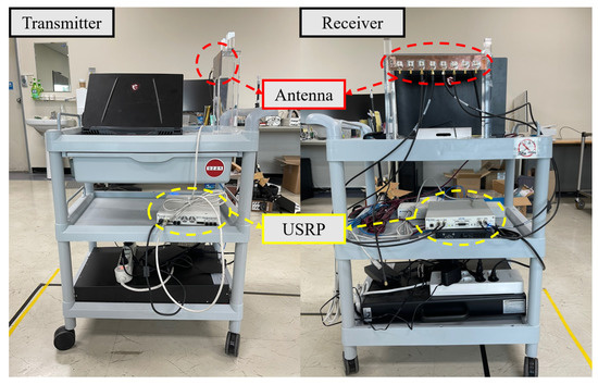
Figure 2.
A picture of transmitter and receiver used for the experiment.
As shown in Figure 3, we data in two different environments, the indoor hallway and the outdoor parking lot. In the indoor hallway, the NLoS signals were expected to be stronger than those in the outdoor parking lot. For this reason, the DoA estimation was expected to be inaccurate in the indoor hallway. DoA estimation range is restricted to since the radiation pattern of each patch antenna in an array is directional. From to in increments, a total of 17,600 covariance matrices were collected, where half of the data were collected in the indoor hallway while the other half weere collected in the outdoor parking lot. During the experiment, the transmitting power was set to 20 dBm, and the distance between transmitter and receiver was fixed to 6 m. With the collected data, the DoA estimation accuracy is analyzed in the following subsection.
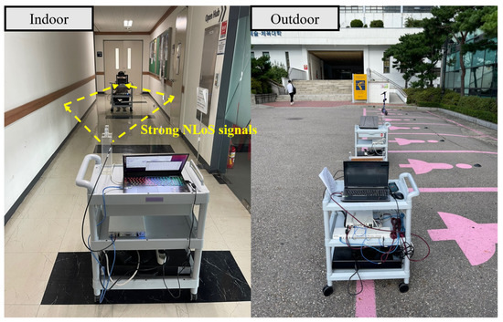
Figure 3.
A picture of the indoor hallway and outdoor parking lot. The NLoS signals were expected to be strong in the indoor hallway.
4.2. Peformance Analysis and Discussion
Before analyzing the DoA estimation performance, we checked the similarity between collected data and synthesized data. Since the DoAs of the multipath signals weere not measured, we compared the collected covariance matrices with ideal covariance matrices. Ideal covariance matrices are the covariance matrices calculated without considering multipath signals and other hardware-induced errors. The ideal covariance matrix is defined as:
where denotes an ideal covariance matrix according to . is a set consisting of labeled DoAs of collected data, which equals .
The correlation between collected covariance matrices and ideal covariance matrices is defined as:
where denotes the correlation according to DoA. denotes the collected covariance matrix whose DoA label is . denotes the correlation between two matrices, which equals . denotes the mean calculated using collected data. , where when can be represented as . Here, a is a constant. Figure 4 shows the correlation between collected covariance matrices and ideal covariance matrices according to DoA and the experiment environment. As expected, the data collected in the indoor environment has a low correlation since it suffers from strong multipath signals. On the other hand, the data collected in the outdoor environment has a higher correlation since there are fewer objects that can make multipath signals.
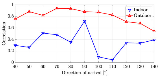
Figure 4.
Correlation between collected covariance matrices and ideal covariance matrices according to DoA and experiment environment.
To analyze the DoA estimation performance, we compared five algorithms. One was MUSIC [2]; two were based on DNN and CNN in Section 3.1, and were trained with 4,000,000 synthesized data. The other two algorithms were also based on DNN and CNN in Section 3.1, but they were trained with 75% of the 17,600 collected data points. When using the collected data for training networks, 25% of the 17,600 collected data points were used for testing DoA estimation accuracy. The root mean squared error (RMSE) is defined as , where and respectively denote the true DoA and the DoA estimated using the test data.
Figure 5 presents two results for the indoor environment, the RMSE of the DoA estimation algorithms and the histogram of estimation results. Both results are derived based on indoor collected data. As expected, Figure 5a,b show that the estimation accuracy is poor in the indoor environment due to the strong NLoS signals. Furthermore, the results also show that the signal model in (2) fails to capture the indoor propagation characteristics since estimation accuracy decreases when using synthesized data for training. However, the DNN and the CNN trained with collected data show much better performance than others. The RMSE of the DNN and the CNN trained with collected data do not surpass in every DoA. To be more specific, Figure 5b shows that estimation results tend to gather around the actual DoA when using collected data. When using synthesized data, however, there is a difference between the mean of estimation results and the actual DoA. Moreover, the variance of the estimation is high.
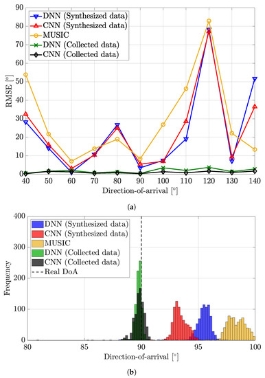
Figure 5.
Performance analysis of DoA estimation algorithms in the indoor environment. The first figure shows the RMSE according to DoA, and the second figure is a histogram of estimation results when the actual DoA is 90°. (a) RMSE. (b) Histogram.
Figure 6 presents two results for the outdoor environment, the RMSE of the DoA estimation algorithms and the histogram of estimation results. Since the NLoS signals are expected to be much weaker in the outdoor environment, the RMSE of all algorithms are much lower than those in Figure 5a. The RMSE tended to increase when the DoA got far from . We think that this is due to the directivity of the antenna elements. The gain of each antenna element was 5 dBi when the DoA was . However, the gain dropped to 2 dBi when the DoA was or . Overall, the DNN trained with synthesized data were more accurate than MUSIC except in a few DoAs, but the RMSE of the CNN trained with synthesized data was unexpectedly high when the DoA was . Meanwhile, the DNN and the CNN trained with collected data were more accurate than others. To be more specific, when using synthesized data, there was a difference between the mean of estimation results and the actual DoA. However, this difference was smaller than that in Figure 5b. When using collected data, estimation results tended to gather around the actual DoA.
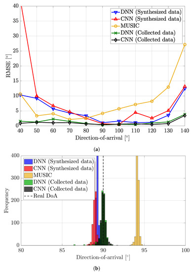
Figure 6.
Performance analysis of DoA estimation algorithms in the outdoor environment. The first figure shows the RMSE according to DoA, and the second figure is a histogram of estimation results when the actual DoA is 90°. (a) RMSE. (b) Histogram.
Table 3 shows a total RMSE of all DoA estimation algorithms. In the indoor environment, the algorithms except those using collected data showed poor performance. Among them, the DNN and CNN trained with synthesized data showed slightly better performance than MUSIC. Although the performance of all algorithms improved in the outdoor, the DNN and CNN trained collected data showed much better performance than others. Since the RMSE of the CNN trained with synthesized data soared when the DoA was —its total RMSE was larger than that of MUSIC.

Table 3.
A total RMSE of DoA estimation algorithms.
Table 4 shows the training time, computation time, and computational complexity of each algorithm. Here, the computational complexity of CNN is derived using [28]. The training time is proportional to the amount of training data. When training a network with 4,000,000 synthesized data points, it took 3500 and 4400 seconds to train the DNN and CNN. On the other hand, it took 190 and 230 seconds to train the DNN and CNN when using collected data points. Although the DNN and CNN-based DoA estimation take a long time for training, their computational complexity is much less than MUSIC once the networks are trained.

Table 4.
Analysis on training time, computation time, and computational complexity.
From all results, we conclude that training with collected data enables accurate DoA estimation. However, collecting sufficient data can be difficult in practice. One of the solutions to this problem is using the synthesized data that well capture the characteristics of the realistic wave. Another solution is to use unsupervised learning such as [20]. Unsupervised learning can make collecting data much easier since data labeling is not required.
5. Conclusions
We present the experimental validation of the deep learning-based DoA estimation using USRP. The DNN and the CNN structures are designed to estimate the DoA of the LoS path with the covariance matrix. In the experiment, two types of data are exploited. One is the data synthesized with the signal model, and the other is the data collected by USRP. The experimental results show that the DoA estimation is most accurate when training DNN and CNN with the collected data. Furthermore, the DoA estimation performance is poor in the indoor environment, which suffers from the strong NLoS signals. However, collecting sufficient data may not be feasible in practice. We expect that this can be resolved by better signal modeling and unsupervised learning.
Author Contributions
Conceptualization, H.C., H.P. and S.K.; methodology, H.C., H.P. and S.K.; software, H.C. and H.P.; validation, H.C., H.P. and S.K.; formal analysis, H.C. and H.P.; investigation, H.C. and H.P.; resources, S.K.; data curation, H.C. and H.P.; writing—original draft preparation, H.C. and S.K.; writing—review and editing, H.C. and S.K.; visualization, H.C. and H.P.; supervision, S.K.; project administration, S.K.; funding acquisition, S.K. All authors have read and agreed to the published version of the manuscript.
Funding
This work was supported by the Future Combat System Network Technology Research Center program of Defense Acquisition Program Administration and Agency for Defense Development (UD190033ED).
Institutional Review Board Statement
Not applicable.
Informed Consent Statement
Not applicable.
Data Availability Statement
Not applicable.
Conflicts of Interest
The authors declare no conflict of interest.
Abbreviations
The following abbreviations are used in this manuscript:
| DoA | Direction-of-arrival |
| USRP | Universal software radio peripheral |
| DNN | Deep neural network |
| CNN | Convolution neural network |
| RNN | Recurrent neural network |
| ResNet | Residual neural network |
| MLE | Maximum likelihood estimation |
| LoS | Line-of-sight |
| NLoS | Non-line-of-sight |
| MUSIC | Multiple signal classification |
| ESPRIT | Estimation of signal parameters via rotational invariance techniques |
| ULA | Uniform linear array |
| MSE | Mean squared error |
| SNR | Signal-to-noise ratio |
| RMSE | Root mean squared error |
References
- Chen, J.C.; Yao, K.; Hudson, R.E. Source localization and beamforming. IEEE Signal Process. Mag. 2002, 19, 30–39. [Google Scholar] [CrossRef]
- Schmidt, R. Multiple emitter location and signal parameter estimation. IEEE Trans. Antennas Propag. 1986, 34, 276–280. [Google Scholar] [CrossRef]
- Roy, R.; Kailath, T. ESPRIT-estimation of signal parameters via rotational invariance techniques. IEEE Trans. Acoust. Speech Signal Process. 1989, 37, 984–995. [Google Scholar] [CrossRef]
- Du, W.; Kirlin, R. Improved spatial smoothing techniques for DOA estimation of coherent signals. IEEE Trans. Signal Process. 1991, 39, 1208–1210. [Google Scholar] [CrossRef]
- Cao, S.; Ye, Z.; Xu, D.; Xu, X. A Hadamard Product Based Method for DOA Estimation and Gain-Phase Error Calibration. IEEE Trans. Aerosp. Electron. Syst. 2013, 49, 1224–1233. [Google Scholar] [CrossRef]
- Ye, Z.; Dai, J.; Xu, X.; Wu, X. DOA Estimation for Uniform Linear Array with Mutual Coupling. IEEE Trans. Aerosp. Electron. Syst. 2009, 45, 280–288. [Google Scholar] [CrossRef]
- Swindlehurst, A.; Kailath, T. A performance analysis of subspace-based methods in the presence of model errors. I. The MUSIC algorithm. IEEE Trans. Signal Process. 1992, 40, 1758–1774. [Google Scholar] [CrossRef]
- Han, F.M.; Zhang, X.D. An ESPRIT-like algorithm for coherent DOA estimation. IEEE Antennas Wirel. Propag. Lett. 2005, 4, 443–446. [Google Scholar] [CrossRef]
- Cadzow, J.; Kim, Y.S.; Shiue, D.C. General direction-of-arrival estimation: A signal subspace approach. IEEE Trans. Aerosp. Electron. Syst. 1989, 25, 31–47. [Google Scholar] [CrossRef]
- Liu, A.; Liao, G.; Zeng, C.; Yang, Z.; Xu, Q. An Eigenstructure Method for Estimating DOA and Sensor Gain-Phase Errors. IEEE Trans. Signal Process. 2011, 59, 5944–5956. [Google Scholar] [CrossRef]
- Chen, P.; Chen, Z.; Cao, Z.; Wang, X. A New Atomic Norm for DOA Estimation With Gain-Phase Errors. IEEE Trans. Signal Process. 2020, 68, 4293–4306. [Google Scholar] [CrossRef]
- Liao, B.; Zhang, Z.G.; Chan, S.C. DOA Estimation and Tracking of ULAs with Mutual Coupling. IEEE Trans. Aerosp. Electron. Syst. 2012, 48, 891–905. [Google Scholar] [CrossRef]
- Lin, M.; Yang, L. Blind Calibration and DOA Estimation With Uniform Circular Arrays in the Presence of Mutual Coupling. IEEE Antennas Wirel. Propag. Lett. 2006, 5, 315–318. [Google Scholar] [CrossRef]
- Kintz, A.L.; Gupta, I.J. A Modified MUSIC Algorithm for Direction of Arrival Estimation in the Presence of Antenna Array Manifold Mismatch. IEEE Trans. Antennas Propag. 2016, 64, 4836–4847. [Google Scholar] [CrossRef]
- Schmidhuber, J. Deep Learning in neural networks: An Overview. Neural Netw. 2015, 61, 85–117. [Google Scholar] [CrossRef]
- Huang, H.; Yang, J.; Huang, H.; Song, Y.; Gui, G. Deep Learning for Super-Resolution Channel Estimation and DOA Estimation Based Massive MIMO System. IEEE Trans. Veh. Technol. 2018, 67, 8549–8560. [Google Scholar] [CrossRef]
- Liu, Z.; Zhang, C.; Yu, P.S. Direction-of-Arrival Estimation Based on Deep Neural Networks With Robustness to Array Imperfections. IEEE Trans. Antennas Propag. 2018, 66, 7315–7327. [Google Scholar] [CrossRef]
- Wu, L.; Liu, Z.; Huang, Z. Deep Convolution Network for Direction of Arrival Estimation With Sparse Prior. IEEE Signal Process. Lett. 2019, 26, 1688–1692. [Google Scholar] [CrossRef]
- Papageorgiou, G.K.; Sellathurai, M.; Eldar, Y.C. Deep Networks for Direction-of-Arrival Estimation in Low SNR. IEEE Trans. Signal Process. 2021, 69, 3714–3729. [Google Scholar] [CrossRef]
- Yuan, Y.; Wu, S.; Wu, M.; Yuan, N. Unsupervised Learning Strategy for Direction-of-Arrival Estimation Network. IEEE Signal Process. Lett. 2021, 28, 1450–1454. [Google Scholar] [CrossRef]
- Mei, R.; Tian, Y.; Huang, Y.; Wang, Z. 2D-DOA Estimation in Switching UCA Using Deep Learning-Based Covariance Matrix Completion. Sensors 2022, 22, 3754. [Google Scholar] [CrossRef] [PubMed]
- Wu, X.; Yang, X.; Jia, X.; Tian, F. A Gridless DOA Estimation Method Based on Convolutional Neural Network With Toeplitz Prior. IEEE Signal Process. Lett. 2022, 29, 1247–1251. [Google Scholar] [CrossRef]
- Merkofer, J.P.; Revach, G.; Shlezinger, N.; van Sloun, R.J.G. Deep Augmented MUSIC Algorithm for Data-Driven DoA Estimation. In Proceedings of the ICASSP 2022—2022 IEEE International Conference on Acoustics, Speech and Signal Processing (ICASSP), Singapore, 23–27 May 2022; pp. 3598–3602. [Google Scholar] [CrossRef]
- de Oliveira, M.L.L.; Bekooij, M.J.G. Deep-MLE: Fusion between a Neural Network and MLE for A Single Snapshot DOA Estimation. In Proceedings of the ICASSP 2022—2022 IEEE International Conference on Acoustics, Speech and Signal Processing (ICASSP), Singapore, 23–27 May 2022; pp. 3673–3677. [Google Scholar] [CrossRef]
- Forster, P.; Larzabal, P.; Boyer, E. Threshold performance analysis of maximum likelihood DOA estimation. IEEE Trans. Signal Process. 2004, 52, 3183–3191. [Google Scholar] [CrossRef]
- Ettus Research. gr-doa. 2019. Available online: https://github.com/EttusResearch/gr-doa (accessed on 26 September 2022).
- Friedlander, B.; Weiss, A. Direction finding in the presence of mutual coupling. IEEE Trans. Antennasm Propag. 1991, 39, 273–284. [Google Scholar] [CrossRef]
- Maji, P.; Mullins, R. On the Reduction of Computational Complexity of Deep Convolutional Neural Networks. Entropy 2018, 20, 305. [Google Scholar] [CrossRef] [PubMed]
Publisher’s Note: MDPI stays neutral with regard to jurisdictional claims in published maps and institutional affiliations. |
© 2022 by the authors. Licensee MDPI, Basel, Switzerland. This article is an open access article distributed under the terms and conditions of the Creative Commons Attribution (CC BY) license (https://creativecommons.org/licenses/by/4.0/).