
Deep Learning-Based Remaining Useful Life Estimation of Bearings with Time-Frequency Information


Abstract
:1. Introduction
2. Related Work
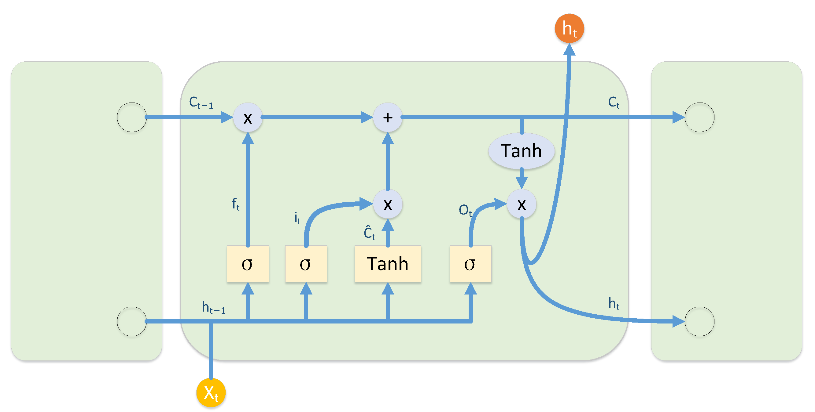
2.1. Long Short-Term Memory
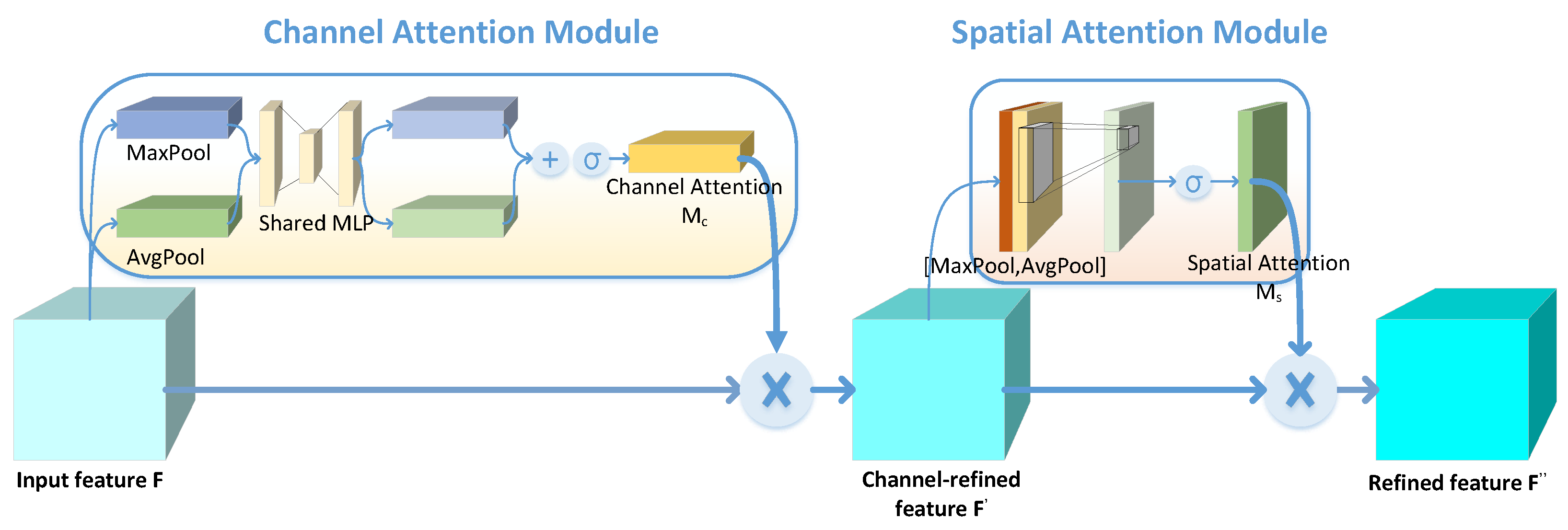
2.2. Convolutional Block Attention Module
3. Framework
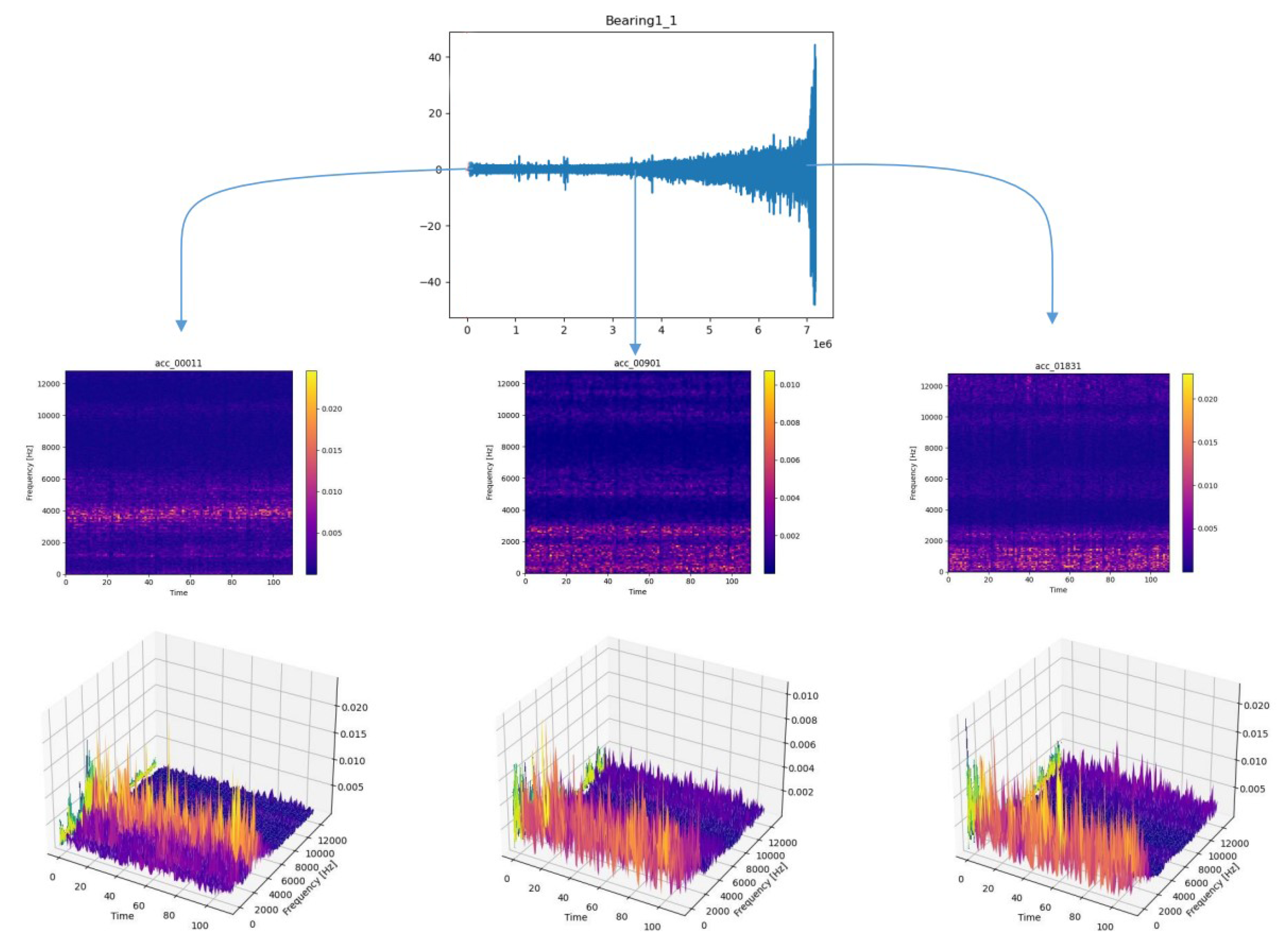
3.1. Vibration Signal Preprocessing
3.2. Network Model Structure
4. Experiments and Discussions
4.1. Data Sets and Evaluation Indicators
4.2. Experimental Setup
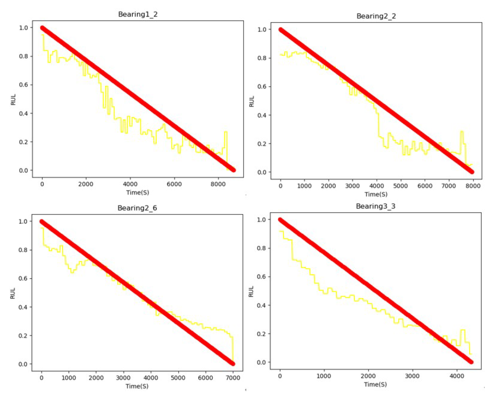
4.3. Analysis
4.4. Feature Information Visualization
5. Summary
Author Contributions
Funding
Institutional Review Board Statement
Informed Consent Statement
Data Availability Statement
Conflicts of Interest
References
- Jouin, M.; Gouriveau, R.; Hissel, D.; Péra, M.C.; Zerhouni, N. Particle filter-based prognostics: Review, discussion and perspectives. Mech. Syst. Signal Process. 2016, 72, 2–31. [Google Scholar] [CrossRef]
- Jouin, M.; Gouriveau, R.; Hissel, D.; Pera, M.C.; Zerhouni, N. Degradations analysis and aging modeling for health assessment and prognostics of PEMFC. Reliab. Eng. Syst. Saf. 2016, 148, 78–95. [Google Scholar] [CrossRef]
- Ali, J.B.; Chebel-Morello, B.; Saidi, L.; Malinowski, S.; Fnaiech, F. Accurate bearing remaining useful life prediction based on Weibull distribution and artificial neural network. Mech. Syst. Signal Process. 2015, 56–57, 150–172. [Google Scholar]
- Soualhi, A.; Medjaher, K.; Zerhouni, N. Bearing Health monitoring based on Hilbert-Huang Transform, Support Vector Machine and Regression. IEEE Trans. Instrum. Meas. 2014, 64, 52–62. [Google Scholar] [CrossRef]
- Aye, S.A.; Heyns, P.S. An integrated Gaussian process regression for prediction of remaining useful life of slow speed bearings based on acoustic emission. Mech. Syst. Signal Process. 2017, 84, 485–498. [Google Scholar] [CrossRef]
- Zhang, Z.; Wang, Y.; Wang, K. Fault diagnosis and prognosis using wavelet packet decomposition, Fourier transform and artificial neural network. J. Intell. Manuf. 2013, 24, 1213–1227. [Google Scholar] [CrossRef]
- Babu, G.S.; Zhao, P.; Li, X.L. Deep Convolutional Neural Network Based Regression Approach for Estimation of Remaining Useful Life. In Proceedings of the International Conference on Database Systems for Advanced Applications, Dallas, TX, USA, 16–19 April 2016. [Google Scholar]
- Ren, L.; Sun, Y.; Wang, H.; Zhang, L. Prediction of Bearing Remaining Useful Life with Deep Convolution Neural Network. IEEE Access 2018, 6, 13041–13049. [Google Scholar] [CrossRef]
- Zhu, J.; Nan, C.; Peng, W. Estimation of Bearing Remaining Useful Life based on Multiscale Convolutional Neural Network. IEEE Trans. Ind. Electron. 2018, 66, 3208–3216. [Google Scholar] [CrossRef]
- Hinchi, A.Z.; Tkiouat, M. Rolling element bearing remaining useful life estimation based on a convolutional long-short-term memory network. Procedia Comput. Sci. 2018, 127, 123–132. [Google Scholar] [CrossRef]
- Wang, B.; Lei, Y.; Yan, T.; Li, N.; Guo, L. Recurrent convolutional neural network: A new framework for remaining useful life prediction of machinery. Neurocomputing 2020, 379, 117–129. [Google Scholar] [CrossRef]
- Li, X.; Zhang, W.; Ding, Q. Deep learning-based remaining useful life estimation of bearings using multi-scale feature extraction. Reliab. Eng. Syst. Saf. 2019, 182, 208–218. [Google Scholar] [CrossRef]
- Elman, J.L. Finding Structure in Time. Cogn. Sci. 1990, 14, 179–211. [Google Scholar] [CrossRef]
- Zaremba, W.; Sutskever, I.; Vinyals, O. Recurrent Neural Network Regularization. arXiv 2014, arXiv:1409.2329. [Google Scholar]
- Woo, S.; Park, J.; Lee, J.Y.; Kweon, I.S. CBAM: Convolutional Block Attention Module. In Proceedings of the European Conference on Computer Vision, Munich, Germany, 8–14 September 2018. [Google Scholar]
- Chui, C.K.; Jiang, Q.; Li, L.; Lu, J. Analysis of an adaptive short-time Fourier transform-based multicomponent signal separation method derived from linear chirp local approximation. J. Comput. Appl. Math. 2021, 396, 113607. [Google Scholar] [CrossRef]
- Sutrisno, E.; Oh, H.; Vasan, A.S.S.; Pecht, M. Estimation of remaining useful life of ball bearings using data driven methodologies. In Proceedings of the 2012 IEEE Conference on Prognostics and Health Management, Denver, CO, USA, 18–21 June 2012; pp. 1–7. [Google Scholar]
- Nectoux, P.; Gouriveau, R.; Medjaher, K.; Ramasso, E.; Chebel-Morello, B.; Zerhouni, N.; Varnier, C. PRONOSTIA: An experimental platform for bearings accelerated degradation tests. In Proceedings of the IEEE International Conference on Prognostics and Health Management, PHM’12, Denver, CO, USA, 18 June 2012; pp. 1–8. [Google Scholar]


| Layer | Parameter | Value |
|---|---|---|
| STFT | Window | Hamming |
| fs | 25,600 Hz | |
| Nperseg | 512 | |
| Conv1 | In channels | 1 |
| Kernel size | 3 × 3 | |
| Out channels | 5 | |
| Conv2 | In channels | 5 |
| Kernel size | 3 × 3 | |
| Out channels | 5 | |
| Conv3 | In channels | 5 |
| Kernel size | 3 × 3 | |
| Out channels | 1 | |
| LSTM | Input size | 1408 |
| Hidden size | 1408 | |
| Num layers | 2 |
| Operating Mode | Radial Force (N) | Rotate Speed (rpm) | Bearing |
|---|---|---|---|
| 1 | 4000 | 1800 | Bearing1-1, Bearing1-2 |
| Bearing1-3, Bearing1-4 | |||
| Bearing1-5, Bearing1-6, Bearing1-7 | |||
| 2 | 4200 | 1650 | Bearing2-1, Bearing2-2 |
| Bearing2-3,Bearing2-4 | |||
| Bearing2-5, Bearing2-6, Bearing2-7 | |||
| 3 | 5000 | 1500 | Bearing3-1, Bearing3-2, Bearing3-3 |
| Bearing | DNN | SSL | SSH | Multi-Scale [12] | SAL-CNN |
|---|---|---|---|---|---|
| Bearing1-1 | 30.4 | 24.3 | 24.4 | 21.4 | 16.9 |
| Bearing1-2 | 28.5 | 17.4 | 22.4 | 14.7 | 13.0 |
| Bearing1-3 | 16.3 | 9.5 | 9.3 | 7.8 | 10.3 |
| Bearing1-4 | 32.1 | 21.3 | 24.5 | 21.8 | 23.0 |
| Bearing1-5 | 28.7 | 21.4 | 19.5 | 18.5 | 11.8 |
| Bearing1-6 | 32.4 | 24.5 | 20.4 | 20.3 | 21.4 |
| Bearing1-7 | 16.6 | 9.6 | 11.7 | 8.3 | 11.9 |
| Bearing2-1 | 28.6 | 24.2 | 25.2 | 21.5 | 18.5 |
| Bearing2-2 | 26.4 | 15.3 | 16.5 | 16.2 | 8.8 |
| Bearing2-3 | 40.5 | 35.2 | 31.5 | 32.8 | 14.8 |
| Bearing2-4 | 22.3 | 11.6 | 9.9 | 6.1 | 24.2 |
| Bearing2-5 | 31.4 | 27.3 | 25.2 | 23.6 | 23.3 |
| Bearing2-6 | 29,4 | 23.2 | 19.8 | 20.7 | 8.6 |
| Bearing2-7 | 38.0 | 28.2 | 28.4 | 27.4 | 27.1 |
| Bearing3-1 | 28.3 | 28.5 | 26.3 | 19.6 | 25.2 |
| Bcaring3-2 | 30.4 | 25.2 | 23.7 | 23.1 | 18.1 |
| Bearing3-3 | 38.5 | 35.4 | 33.5 | 30.4 | 11.1 |
| Bearing | Image Type | Early Stage | Middle Stage | Late Stage |
|---|---|---|---|---|
| 1-1 | Time-frequency graph |  | 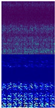 | 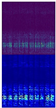 |
| Heatmap | ||||
| 1-3 | Time-frequency graph | 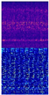 | 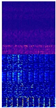 | 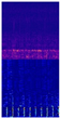 |
| Heatmap | ||||
| 1-5 | Time-frequency graph |  |  | 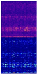 |
| Heatmap |
Publisher’s Note: MDPI stays neutral with regard to jurisdictional claims in published maps and institutional affiliations. |
© 2022 by the authors. Licensee MDPI, Basel, Switzerland. This article is an open access article distributed under the terms and conditions of the Creative Commons Attribution (CC BY) license (https://creativecommons.org/licenses/by/4.0/).
Share and Cite
Liu, B.; Gao, Z.; Lu, B.; Dong, H.; An, Z. Deep Learning-Based Remaining Useful Life Estimation of Bearings with Time-Frequency Information. Sensors 2022, 22, 7402. https://doi.org/10.3390/s22197402
Liu B, Gao Z, Lu B, Dong H, An Z. Deep Learning-Based Remaining Useful Life Estimation of Bearings with Time-Frequency Information. Sensors. 2022; 22(19):7402. https://doi.org/10.3390/s22197402
Chicago/Turabian StyleLiu, Bingguo, Zhuo Gao, Binghui Lu, Hangcheng Dong, and Zeru An. 2022. "Deep Learning-Based Remaining Useful Life Estimation of Bearings with Time-Frequency Information" Sensors 22, no. 19: 7402. https://doi.org/10.3390/s22197402
APA StyleLiu, B., Gao, Z., Lu, B., Dong, H., & An, Z. (2022). Deep Learning-Based Remaining Useful Life Estimation of Bearings with Time-Frequency Information. Sensors, 22(19), 7402. https://doi.org/10.3390/s22197402