Stability Analysis of Two Power Converters Control Algorithms Connected to Micro-Grids with Wide Frequency Variation

Abstract

Distributed power generation, micro-grids, and networks working in islanding mode have strong deviations in voltage quantities. These deviations can be divided into amplitude and frequency. Amplitude deviations are well-known and studied, as they are common in small and big grids. However, deviations on the ac mains frequency have not been widely studied. The literature shows control schemes capable of bearing these variations, but no systematic analysis has been performed to ensure stability. As the majority of power converters are designed for big grids, their analysis and design neglect frequency disturbances, therefore those devices allow a very small frequency operating window. For instance, in power converters that need to be synchronized to the grid, the standard deviation does not go beyond 0.5 Hz, and for grid-tied inverters it does not go beyond 1 Hz, whereas variations of around 8 Hz can be expected in micro-grids. This work presents a comprehensive analysis of the control system’s stability, where two different control schemes for a back-to-back static converter topology are implemented and studied under a wide variable grid frequency. Because the behavior of power converters is nonlinear and coupled, dynamic and static decouplers are usually introduced in the controller, being a key element on the scheme according to the findings. The results show that using just a static decoupler does not guarantee stability under frequency variations; meanwhile, when a dynamic decoupler is used, the operating window can be greatly extended. The procedure shown in this paper can also be extended to other control algorithms, making it possible to carefully choose the control system for a variable frequency condition. Simulated and experimental results confirm the theoretical approach.

1. Introduction

Certainly, due to the proliferation of distributed generation, micro-grids, islanded systems, and non-conventional power generation sources, grid frequency variation has become a topic for research and study. These sources, for instance, in aircraft and others applications, present important changes in their operating conditions, particularly concerning frequency, which may deviate as far as 75%, as shown in [1], or even 100% as shown in [2,3,4,5]. In addition, significant fluctuations in generating conditions are normal in wind power turbines and weak power systems (−12%, +8%) [6,7,8,9], and are also present as critical frequency variation ranges for normal power systems (−6%, +4%) [10] in contrast to conventional stiff and high power grids in normal operation frequency variation ranges (±1%) [10]. In addition, power systems working in islanding mode, as well as ship power systems, are also of interest, where large variations in the fundamental frequency are part of the normal operating conditions. In addition, many aircraft power systems are designed for a wide-frequency environment in order to obtain a suitable response for these kinds of disturbances [2,3,4,5].

The increasing performance requirements placed on grid synchronization for proper converter operation under varying conditions has given rise to improved discrete Phase-Locked Loops (PLLs) schemes. Many of these synchronization methods have been developed to operate under variable frequency conditions [5,11,12,13,14,15,16,17,18,19], and can operate correctly even under both polluted [5,15,19,20,21] and unbalanced ac voltages [22]. They can be readily utilized in several power electronics systems’ applications, being of particular interest for grid-connected power converters such as [23,24,25,26,27,28], given that their use on these power converters is mandatory for adequate operation [1,13,19,29,30]. From the control point of view, frequency and phase synchronization is critical for synchronous reference frame (SRF)-based controllers, due to their reliance on accurate variable transformations used in the control loops [5]. Although these algorithms allow the estimation of the grid frequency with a good degree of accuracy [1,2,3,4,5,6,7,8,9,10,11,12,13,14], the effects of a variable grid frequency are often neglected or not explicitly considered in the design of the power converter control loops [31,32]. However, when weak power systems are considered, or when the system is operating in islanding mode, variation in the system frequency is to be expected [1,2,3,4,5,8,9].

Regarding the design of power converter control loops, the most common scheme, used for instance on active rectifiers, is designed as a master loop controlling the dc link voltage and power factor, which gives the current or power reference to an inner control loop. However, due to the high degree of coupling in the inner loop, decouplers are mandatorily included in order to induce a single-input and single-output behavior. Decouplers can be classified as static [33] and dynamic [34,35,36]. Static decouplers are a simple and appealing alternative because sensors and mathematical calculations are reduced, leading to a lowered computational effort. This is an important feature, especially in multilevel converters where the controllers have a higher complexity. On the other hand, dynamic decouplers have also been widely used in power electronics applications because they have a better performance and behavior, but with additional computational costs and the need to sense more variables and estimate the system’s parameters.

The typical approach used to control grid-connected power converters is to consider a constant grid frequency [32,34,35,36,37], meaning that a static decoupler is implicitly adopted; however, if the grid frequency is not constant, the model ceases to represent the true system dynamics. For instance, controller design of three-phase power converters is usually carried out in a rotating dq reference frame. During this process, the electrical system’s frequency is typically considered as a fixed parameter. Then, controller tuning is performed to achieve the desired performance specifications, such as settling time, damping factor, and, most importantly, stability. However, after the controller design is complete, its parameters are left fixed, thus neglecting the significant variation in the electrical system’s frequency that can be present during operation. Therefore, a systematic study of the effect of frequency variation on the behavior of the control system is required. In this way, the issue of variable grid frequency can determine when the controllers, based on dynamic or static decoupler, are valid, or, more strictly, stable in a wide variable frequency environment.

This paper presents a comprehensive analysis of the stability of the control system in one of the most common grid-tied converters under variations in grid frequency. As cases of study, this work studies the behavior of the most commonly used dq SRF-based control methods as applied in three-phase grid-connected boost rectifiers, obtaining how far the frequency may deviate from design values without affecting the system’s control loops in terms of stability. In addition, it gives guidelines to assess the stability, which may be extended to other topologies where frequency variation is expected. In particular, the main contribution of this paper is a systematic procedure to quantify the stability range of well-known dq SRF-based control schemes that use static and dynamic decouplers such as [35,36,38]. Theoretical and experimental results are included in a proof-of-concept prototype in order to validate the proposed analysis.

The analysis first considers the study of a SRF-based linear controller with a static decoupler [39]. Then, a second one is analyzed, this time based on a dynamic decoupler, which explicitly includes the time-variant feature of the ac mains frequency. An analysis is performed for the static and dynamic decoupler through the Lyapunov stability criteria to find the eigenvalues considering a micro-grid with variable frequency and, thus, conclude stability issues under the aforementioned considerations.

The paper is organized as follows. Section 2 presents the model of the power converter under variable grid frequency. Section 3 presents the control algorithms with the decouplers. Section 4 shows the theoretical stability analysis for the controllers. Section 5 shows simulated results which illustrate the issues. Section 6 shows experimental results which validate the theoretical analysis. Section 7 discusses the results. Finally, Section 8 indicates the main conclusions from this study.

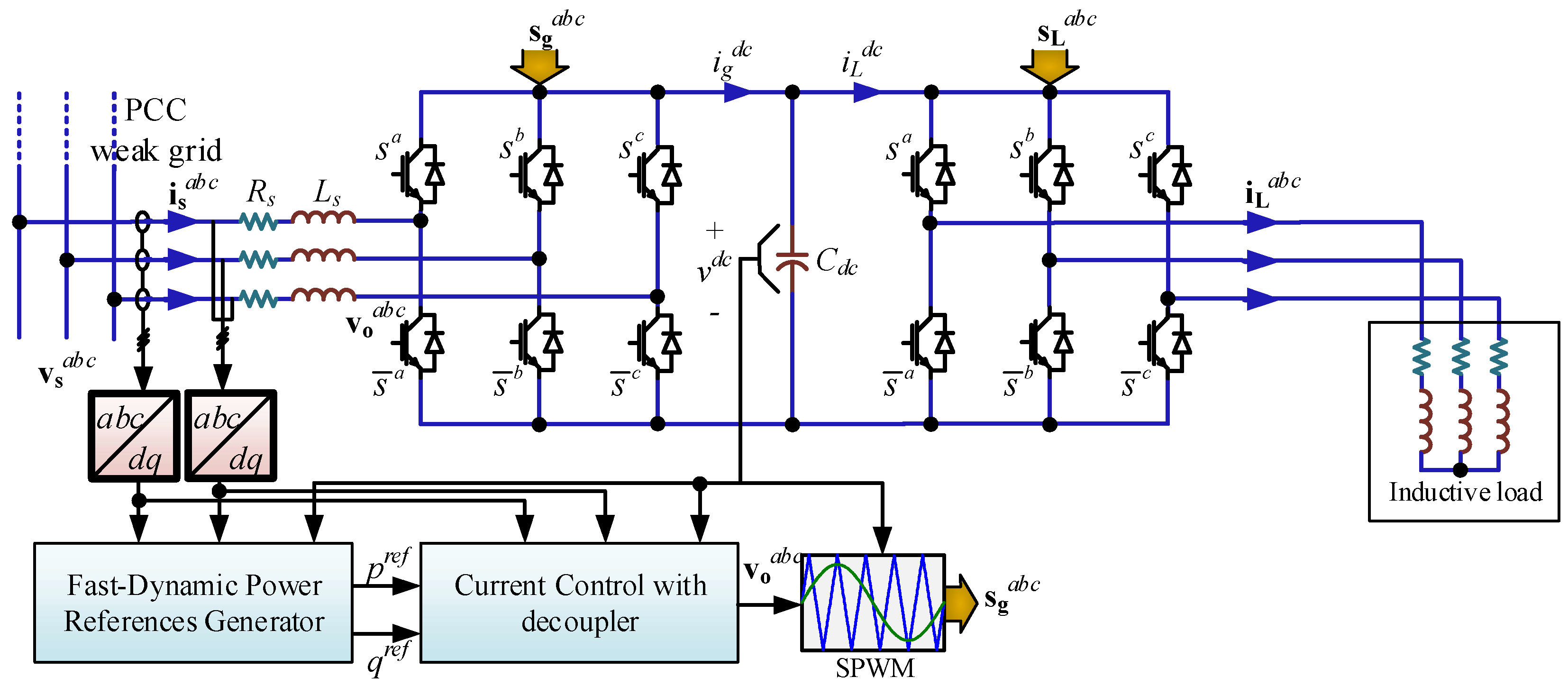
2. Modeling of Power Converters under Variable Grid Frequency

The grid-connected power converter can be modeled by explicitly considering a variable grid frequency [4,22]. The rectifier side of the system shown in Figure 1 is modeled through the Kirchhoff’s current and voltage laws, resulting in

$$C_{dc}\frac{d{v}^{dc}}{dt}=i_g{}^{dc}-i_L{}^{dc}=G_{ac}\left({({\mathbf{m}}_{\mathbf{g}}{}^{abc})}^T{\mathbf{i}}_{\mathbf{g}}{}^{abc}-{({\mathbf{m}}_{\mathbf{L}}{}^{abc})}^T{\mathbf{i}}_{\mathbf{L}}{}^{abc}\right)$$

(1)

$${\mathbf{v}}_{\mathbf{g}}{}^{abc}=L_g\frac{d{\mathbf{i}}_{\mathbf{g}}{}^{abc}}{dt}+R_g{\mathbf{i}}_{\mathbf{g}}{}^{abc}+G_{ac}{\mathbf{m}}_{\mathbf{g}}{}^{abc}{v}^{dc}$$

(2)

where G_ac is the modulation technique gain (G_ac = 0.866 for plain sinusoidal PWM), m_g^abc and m_L^abc are the rectifier and the inverter modulating signals, respectively.

Equations (1) and (2) can be rewritten in the rotating reference frame by the use of the Park Transformation, leading to the following state variable equations:

$$\frac{d{v}^{dc}}{dt}=\frac{G_{ac}}{C_{dc}}\left(m_g{}^d{i}_g{}^d+m_g{}^q{i}_g{}^q\right)-\frac{1}{C_{dc}}{i}_L^{dc}$$

(3)

$$\frac{d{i}_g{}^d}{dt}=\frac{-R_g}{L_g}{i}_g{}^d+{\omega }_g{i}_g{}^q-\frac{1}{L_g}{G}_{ac}{m}_g{}^d{v}^{dc}+\frac{1}{L_g}{v}_g{}^d$$

(4)

$$\frac{d{i}_g{}^q}{dt}=\frac{-R_g}{L_g}{i}_g{}^q-{\omega }_g{i}_g{}^d-\frac{1}{L_g}{G}_{ac}{m}_g{}^q{v}^{dc}+\frac{1}{L_g}{v}_g{}^q$$

(5)

where ω_g is the variable grid frequency in rad/s. The model shows a new nonlinearity due to the frequency ω_g, which is considered as a disturbance on the currents i_g^d and i_g^q in (4) and (5), respectively. This nonlinearity requires a careful choice of control technique in order to obtain proper dynamic and static behavior.

In order to simplify the mathematical analysis, the state function f is defined after writing (3)–(5) in the standard nonlinear system form as

$$dx/dt=\mathbf{f}\left(\mathbf{x},\mathbf{u},\mathbf{p}\right)$$

(6)

where x = [v^dc i_g^d i_g^q]^T, u = [m_g^d m_g^q]^T, p = [v_g^d v_g^q ω_g i_L^dc]^T for the rectifier control side. The disturbances are the grid voltage and frequency, and the dc current of the inverter side. A more detailed analysis of the system model can be found in [38].

3. Control of Power Converters under Variable Grid Frequency

The system in Figure 1 shows a variable frequency voltage source, but a constant frequency is desired at the load side. This topology can be found on micro-grids where the frequency may deviate from the operating point, but the load requires a fixed frequency.

3.1. Control Goals

Two control techniques are used to operate the system in Figure 1, when a variable frequency environment is considered: (i) SRF linear controller with a static decoupler, and (ii) SRF linear controller with dynamic decoupler based on state variables and disturbances feed-forward. Both controllers have the same objectives, which are to control the active power (to regulate the dc voltage) and the reactive power (to regulate the grid power factor). The dc link voltage can be controlled by the direct axis current and the power factor through the quadrature current.

3.2. Linear Control with Static Decoupler

The first case of study uses linear controllers with a static decoupler, which is designed for a specific operating point. To obtain the static decoupler, the linear model must be found from (6) [33], given by:

$$\Delta \dot{x}=A\Delta x+B\Delta u+E\Delta p$$

(7)

with:

$$A=\frac{df\left(x_o,u_o,p_o\right)}{dx};B=\frac{df\left(x_o,u_o,p_o\right)}{du};E=\frac{df\left(x_o,u_o,p_o\right)}{dp}$$

(8)

the linear system matrices, and Δx = x − x_o, Δu = u − u_o, Δp = p − p_o, the state variables. The inputs and the disturbances associated with a chosen operating point are described by the subscript ‘_o’.

From the current control point of view, i_g^d and i_g^q are the variables of interest. Hence, the output vector, namely y, can be written as:

$$\Delta y=C\Delta x=\left(\begin{array}{ccc}0& 1& 0\\ 0& 0& 1\end{array}\right)\left(\begin{array}{c}{v}_{dc}-v_{dc}{}_o\\ i_g^d-i_g^d{}_o\\ i_g^q-i_g^q{}_o\end{array}\right)$$

(9)

From (8) and (9), the Matrix Transfer Function, which gives the linear representation [40], becomes:

$$\mathbf{H}\left(s\right)=\mathbf{C}{\left(s\mathbf{I}-\mathbf{A}\right)}^{-1}\mathbf{B}$$

(10)

and the static decoupler [33] is:

$$\begin{array}{l}{\mathbf{H}}^{-1}\left(0\right)=-{\left(\mathbf{C}{\mathbf{A}}^{-1}\mathbf{B}\right)}^{-1}\\ =\frac{\left(\begin{array}{cc}{\left(m_g^d{}_o\right)}^2{v}_{dc}{}_o+{\alpha }_1& m_g^d{}_o{m}_g^q{}_o{v}_{dc}{}_o+{\alpha }_2\\ m_g^d{}_o{m}_g^q{}_o{v}_{dc}{}_o+{\alpha }_3& {\left(m_g^q{}_o\right)}^2{v}_{dc}{}_o+{\alpha }_4\end{array}\right)}{G_{ac}\left(i_g^d{}_o{m}_g^d{}_o+i_g^q{}_o{m}_g^q{}_o\right)v_{dc}{}_o}\end{array}$$

(11)

where:

$${\alpha }_1=-L_g{i}_g^q{}_o{m}_g^d{}_o{\omega }_g{}_o+R_g{i}_g^q{}_o{m}_g^q{}_o,{\alpha }_2=-L_g{i}_g^q{}_o{m}_g^q{}_o{\omega }_g{}_o-R_g{i}_g^q{}_o{m}_g^d{}_o,{\alpha }_3=L_g{i}_g^d{}_o{m}_g^d{}_o{\omega }_g{}_o-R_g{i}_g^d{}_o{m}_g^q{}_o,{\alpha }_4=L_g{i}_g^d{}_o{m}_g^q{}_o{\omega }_g{}_o+R_g{i}_g^d{}_o{m}_g^d{}_o.$$

Note that all the quantities in H⁻¹(0) are chosen for a specific operating point.

The static decoupler (11), designed for a certain operating point, provides a decoupled current control in steady state. Therefore, in order to achieve zero steady state error, two independent Proportional-Integral (PI) controllers are used with the form:

$$h_c\left(s\right)=k_p^{i_g}\left(1+\frac{1}{T_i^{i_g}s}\right)$$

(12)

where k_p is the proportional gain and T_i is the integrative time. These PI controllers are also designed for a specific operating point to obtain a desired dynamic and static performance for a fixed frequency ω_go [33,34]. The control system scheme is shown in Figure 2, including the dc voltage and the power factor control loops.

3.3. Linear Control with Dynamic Decoupler

A dynamic decoupler is another option to linearize and decouple the system [33]. Similar to the static decoupler case, the dc voltage control is a master loop on the direct current, while the required power factor gives the quadrature current reference.

The dynamic decoupler is found deriving the equation that defines the output variables and making them equal to new input variables that herein are named w₁ and w₂:

$$\frac{d{i}_g^d}{dt}=w_1,\frac{d{i}_g^q}{dt}=w_2$$

(13)

where the left side in the last equations are (4) and (5). Thus, from (4), (5) and (13), it is found:

$$\frac{d{i}_g^d}{dt}=\frac{-R_g}{L_g}{i}_g{}^d+{\omega }_g{i}_g{}^q-\frac{1}{L_g}{G}_{ac}{m}_g{}^d{v}^{dc}+\frac{1}{L_g}{v}_g{}^d=w_1$$

(14)

$$\frac{d{i}_g^q}{dt}=\frac{-R_g}{L_g}{i}_g{}^q-{\omega }_g{i}_g{}^d-\frac{1}{L_g}{G}_{ac}{m}_g{}^q{v}^{dc}+\frac{1}{L_g}{v}_g{}^q=w_2$$

(15)

and solving for m_g^d and m_g^q, the resulting dynamic decoupler to be implemented is:

$$m_g^d={\left(G_{ac}{v}^{dc}\right)}^{-1}\left\{-L_g{w}_1-R_g{(i_g^d)}^i+L_g{\omega }_g^i{(i_g^q)}^i+{(v_g^d)}^i\right\}$$

(16)

$$m_g^q={\left(G_{ac}{v}^{dc}\right)}^{-1}\left\{-L_g{w}_2-R_g{(i_g^q)}^i-L_g{\omega }_g^i{(i_g^d)}^i+{(v_g^q)}^i\right\}$$

(17)

where the superscript i means that the variable is obtained from the Park Transformation, which uses the frequency estimated by the PLL and may be different from the real variable. Indeed, the Park Transformation angular position θⁱ given by the PLL is an estimation of the real angle position θ.

With the dynamic decoupler defined in (16) and (17), the system defined by the current i_g^{d,q} and the input w_{1,2} behaves as an integrator. In order to obtain a first order linear response (h(s) = k_p/(τs + 1) = i_g^{d,q}/v_{1,2}), the inputs w₁ and w₂ are redefined as:

$$w_1=\left(1/\tau \right){(i_g^d)}^i+k_p\left(1/\tau \right)v_1$$

(18)

$$w_2=\left(1/\tau \right){(i_g^q)}^i+k_p\left(1/\tau \right)v_2$$

(19)

where v = [v₁ v₂]^T is the new input vector to impose a first order response. Finally, the modulation signals are:

$$m_g^d=\frac{-\frac{L_g}{\tau }\left(-{\left(i_g^d\right)}^i+k_p{v}_1\right)-R_g{\left(i_g^d\right)}^i+L_g{\omega }_g^i{\left(i_g^q\right)}^i+{\left(v_g^d\right)}^i}{G_{ac}{v}^{dc}}$$

(20)

$$m_g^q=\frac{-\frac{L_g}{\tau }\left(-{\left(i_g^q\right)}^i+k_p{v}_2\right)-R_g{\left(i_g^q\right)}^i-L_g{\omega }_g^i{\left(i_g^d\right)}^i+{\left(v_g^q\right)}^i}{G_{ac}{v}^{dc}}$$

(21)

Equations (20) and (21) show ${\omega }_g^i$ as a necessary variable to implement the dynamic decoupler, with ${\omega }_g^i$ being the estimated angular frequency of the ac mains. This frequency is obtained from the PLL [5,22], as:

$${\omega }_g^i=2\pi /\left(N{T}_s\right)$$

(22)

Note that the PLL ensures ${\omega }_g^i$ equal to ${\omega }_g$ in a steady state and it is a good approximation during transient conditions [1,2,3,4,5,6,7,8,9,10,11,12,13,14]. Moreover, in this work, the ac mains frequency is estimated at every sampling time by means of a discrete three-phase SRF PLL. This approach also guarantees a fixed number N of samples per period, as the sampling time T_s is also adjusted [3,5].

The SRF variables in (20) and (21), which are identified by the superscript i, also denotes the dq variables obtained from the Park Transformation. The relationship between the real x (voltage or current) and the estimated xⁱ is:

$${\left(x^d\right)}^i=\sqrt{{(x^d)}^2+{(x^q)}^2}\cos \left({\theta }^i-\theta +{\tan }^{-1}\left(\frac{x^q}{x^d}\right)\right)$$

(23)

$${\left(x^q\right)}^i=\sqrt{{(x^d)}^2+{(x^q)}^2}\sin \left({\theta }^i-\theta +{\tan }^{-1}\left(\frac{x^q}{x^d}\right)\right)$$

(24)

Naturally, if θⁱ = θ, i.e., the PLL is in a steady state, then (x^d)ⁱ = x^d and (x^q)ⁱ = x^q. It is important to highlight that the difference between the real and the estimated variable is small, since PLLs are now very accurate [1,2,3,4,5,6,7,8,9,10,11,12,13,14]. This justifies assuming both variables are identical for control design and analysis.

Finally, a similar control structure of the static decoupler, Figure 2, is applied to the designed dynamic decoupler as shown in Figure 3, controlling both the dc link voltage and the power factor by means of a PI controller. For discrete control implementation, the PI controllers of Figure 2 and Figure 3 must be mapped to the Z-plane, as explained in [37,38].

4. Stability Analysis Procedure

An important issue about the previous controllers is their stability within a certain range of frequency and/or their operation in the presence of frequency deviations for applications such as micro-grids and weak grids, among others. The open loop model (6) is a nonlinear and coupled system, therefore the Lyapunov stability criteria can be used to study the effect of frequency variations.

4.1. Stability Analysis of Static Decoupler Control

The static decoupler is computed for a nominal operating point, but this condition, especially the frequency, could shift away from the original value and lead to an unstable control system. This is expected because the decoupler depends on the state variables, inputs, disturbances, and parameters (11), besides the frequency at the operating point. In order to analyze the system response under grid frequency variations, a stability study is performed in this section for the global closed loop system shown in Figure 2.

The modulating signals, depending upon the current controller outputs and the static decoupler, can be written as:

$$\left(\begin{array}{c}\Delta m_g^d\\ \Delta m_g^q\end{array}\right)={\mathbf{H}}^{-1}\left(0\right)\left(\begin{array}{c}{v}_1\\ v_2\end{array}\right)=\mathbf{K}\left(\begin{array}{c}{v}_1\\ v_2\end{array}\right)=\left(\begin{array}{cc}{k}_{11}& k_{12}\\ k_{21}& k_{22}\end{array}\right)\left(\begin{array}{c}{v}_1\\ v_2\end{array}\right)$$

(25)

where $\Delta m_g^{\left\{d,q\right\}}=m_g^{\left\{d,q\right\}}-m_g^{\left\{d,q\right\}}{}_o$.

As it was stated in Section 4, the quadrature current reference is given by the desired input power factor, and the direct current is given by the dc voltage control output. Because both current control loops use a PI controller (12), the current control state variables representation of (12) can be written as:

$${\dot{\zeta }}_1=a_c{\zeta }_1+b_c\left({\left(i_g^d\right)}^{ref}-i_g^d\right),v_1=c_c{\zeta }_1+d_c\left({\left(i_g^d\right)}^{ref}-i_g^d\right)$$

(26)

$${\dot{\zeta }}_2=a_c{\zeta }_2+b_c\left({\left(i_g^q\right)}^{ref}-i_g^q\right),v_2=c_c{\zeta }_2+d_c\left({\left(i_g^q\right)}^{ref}-i_g^q\right)$$

(27)

where a_c = 0, b_c = 1, c_c = k_c/T_i, d_c = k_c are the current controller parameters. On the other hand, the PI for the dc voltage control can be expressed as:

$$\begin{array}{l}{\dot{\zeta }}_3=a_c^{v^{dc}}{\zeta }_3+b_c^{v^{dc}}\left({\left(v_{}^{dc,ref}\right)}^2-{\left(v^{dc}\right)}^2\right),\\ {\left(i_g^d\right)}^{ref}=c_c^{v^{dc}}{\zeta }_3+d_c^{v^{dc}}\left({\left(v_{}^{dc,ref}\right)}^2-{\left(v^{dc}\right)}^2\right)\end{array}$$

(28)

where a_c^vdc = 0, b_c^vdc = 1, c_c^vdc = k_c/T_i, d_c^vdc = k_c are the voltage controller parameters.

Using the state variables representation of the current controller (26) and (27) and the dc voltage controller (28), the overall closed loop system model can be written in the state variable form. This is defined by the union (closed loop, Figure 2) of the open loop model (3)–(5), the static decoupler (25), the current controller (26) and (27) and the dc voltage controller (28) in one equation, leading to the following nonlinear state variable representation [38,41]:

$$\frac{d{\mathbf{x}}_L}{dt}={\mathbf{f}}_{\mathbf{L}}\left({\mathbf{x}}_L,u_L,{\mathbf{p}}_L\right)$$

(29)

where $x_L={[v^{dc},i_g^d,i_g^q,{\zeta }_1,{\zeta }_2,{\zeta }_3]}^T$, and $u_L={[{(v_{}^{dc,ref})}^2,{(i_g^q)}^{ref}]}^T$. The stability of the resulting system (29) can be studied applying Lyapunov’s method, which verifies the eigenvalues in each operating point of the Jacobian matrix:

$${\mathbf{A}}_{\mathbf{L}}=\frac{\partial {\mathbf{f}}_{\mathbf{L}}\left({\mathbf{x}}_L,u_L,{\mathbf{p}}_L\right)}{\partial {\mathbf{x}}_L}$$

(30)

The passive filtering components utilized in the topology, Figure 1, are designed considering the switching frequency and further details are given in [40]. For the eigenvalues study, a power factor at the source of pf_g = 0.93(i) and a dc voltage v^dc = 750 (V) with grid frequencies from 30 (Hz) to 100 (Hz) are imposed. Figure 4 shows the eigenvalues with the parameters given in

Table 1. System parameters.

Parameters	Value	P.U.
vg	220 V, rms	1
vdc	750 V	3.4
ZL (50 Hz)	8.8 Ω	1
RL (50 Hz)	7 Ω	0.80
LL (50 Hz)	17 mH	0.61
Rg (50 Hz)	0.1 Ω	0.011
Lg (50 Hz)	12 mH	0.43
Cdc (50 Hz)	4.7 mF	0.36
fg	50 Hz	1
fsw	1.05 kHz	21
N	204	--
kc (current)	1.0	--
Ti (current)	20 m	--
kc (dc voltage)	0.070	--
Ti (dc voltage)	0.10	--

. Figure 4b highlights the eigenvalues nearest to the imaginary axis, where the critical grid frequency is 81.7 Hz. It is worth noting that the value of the critical frequency is strongly dependent on the parameters and the operating point, as shown in

Table 2. Critical frequency for static decoupler.

Parameters	Value	Critical Frequency
Lg	70%	Over 100 Hz
	nominal	81.7 Hz
	130%	62.4 Hz
Rg	70%	81.2 Hz
	nominal	81.7 Hz
	130%	82.2 Hz
Cdc	70%	82.4 Hz
	nominal	81.7 Hz
	130%	81.1 Hz

in percentage with respect the nominal value. However, the most variation in the critical frequency is related to the inductance value, and, on the contrary, the losses in the inductances (the resistance R_g) are the ones that less affect the stable zone. This is highlighted in Figure 5, where Figure 5a shows the response for L_g, where the higher the value of L_g is, the lower the critical frequency is (where the eigenvalues are equal to zero). On the other hand, Figure 5b,c shows critical frequency little dependence with respect to R_g and C_dc.

As aforementioned, high frequencies lead some eigenvalues to reach positive real values, making the closed loop system unstable, as confirmed in the next section. The eigenvalues that become unstable for high frequencies are the ones given by the first order L-type input filter that are defined by the impedance R_g + jω_gL_g. These eigenvalues are already very close to the imaginary axis in open loop because R_g → 0, where R_g represents the resistive losses of the filter. Moreover, the imaginary part is related to the ac mains frequency.

4.2. Stability Analysis of Dynamic Decoupler Control

The error introduced by the PLL was not considered in the stability analysis of the linear control with a static decoupler because the control strategy is unstable even when an ideal PLL is considered. On the other hand, the error introduced by the PLL in the linear control with a dynamic decoupler needs to be considered because the nonlinear feedback uses the estimated frequency, affecting the overall performance.

The analysis was carried out in the continuous domain to reduce the mathematical burden, thus, the PLL is considered as a second order transfer function, h_PLL(s) = ω_n²/(s² + 2ξω_ns + ω_n²), which should represent as close as possible the PLL response. Hence, the PLL state variables representation can be written as:

$$\frac{d{\delta }_1}{dt}={\delta }_2$$

(31)

$$\frac{d{\delta }_2}{dt}=-{\omega }_n{}^2{\delta }_1-2\xi {\omega }_n{\delta }_2+{\omega }_n{}^2\frac{1}{N\cdot f_g}$$

(32)

where ω_n is the PLL natural frequency and ξ is the PLL damping factor. The variable f_g is the real grid frequency and δ₁ = T_s, where the estimated frequency can be found as (22).

To study the global system stability, the dynamic decoupler must be included, which leads to applying the dynamic decoupler (20) and (21) in the system model given by (3)–(5), resulting in (33)–(35):

$$\frac{d{i}_g{}^d}{dt}=\frac{-1}{\tau }{\left(i_g^d\right)}^i+\frac{k_p}{\tau }{v}_1+\frac{-R_g}{L_g}\left(i_g^d-{\left(i_g^d\right)}^i\right)+\left({\omega }_g{i}_g^q-\frac{{\left(i_g^q\right)}^i}{N{T}_s}\right)+\frac{1}{L_g}\left(v_g^d-{\left(v_g^d\right)}^i\right)$$

(33)

$$\frac{d{i}_g{}^q}{dt}=\frac{-1}{\tau }{\left(i_g^q\right)}^i+\frac{k_p}{\tau }{v}_2+\frac{-R_g}{L_g}\left(i_g^q-{\left(i_g^q\right)}^i\right)-\left({\omega }_g{i}_g^q-\frac{2\pi {\left(i_g^q\right)}^i}{N{T}_s}\right)+\frac{1}{L_g}\left(v_g^q-{\left(v_g^q\right)}^i\right)$$

(34)

$$\frac{d{v}^{dc}}{dt}=\frac{G_{ac}}{C_{dc}}\left(\begin{array}{l}\frac{1}{G_{ac}{v}^{dc}}\left\{\begin{array}{l}-L_g\left(\left(-1/\tau \right){\left(i_g^d\right)}^i+\left(k_p/\tau \right)v_1\right)-R_g{\left(i_g^d\right)}^i+\cdots \\ L_g\left(2\pi /\left(N{T}_s\right)\right){\left(i_g^q\right)}^i+{\left(v_g^d\right)}^i\end{array}\right\}{i}_g^d+\cdots \\ \frac{1}{G_{ac}{v}^{dc}}\left\{\begin{array}{l}-L_g\left(-1/\tau \right){\left(i_g^q\right)}^i+\left(k_p/\tau \right)v_2-R_{g}i{\left(i_g^q\right)}^i+\cdots \\ -L_g\left(2\pi /\left(N{T}_s\right)\right){\left(i_g^d\right)}^i+{\left(v_g^q\right)}^i\end{array}\right\}{i}_g^q\end{array}\right)-\frac{1}{C_{dc}}{i}_L{}^{dc}$$

(35)

At this point, the effect of the sampling time T_s shows up, because if ${\omega }_g=2\pi /\left(N{T}_s\right)$ (when the PLL is perfectly synchronized), all parenthesis in (33) and (34) add up to zero, and the dynamic decoupler obtains the desired time constant τ between i_g and v (just the two first terms).

Then, including the state variables related to the PLL (31) and (32), the open loop system (3)–(5) and the PI controllers (26)–(28), the state variable representation for the overall closed loop system with nonlinear control is summarized in (36),

$$d{\mathbf{x}}_{NL}/dt={\mathbf{f}}_{N\mathbf{L}}\left({\mathbf{x}}_{NL},u_{NL},{\mathbf{p}}_{NL}\right)$$

(36)

with ${\mathbf{x}}_{NL}^T=[{\delta }_1,{\delta }_2,v_{}^{dc},i_g^d,i_g^q,{\zeta }_1,{\zeta }_2,{\zeta }_3]$, ${\mathbf{p}}_{NL}^T=[v_g^d,v_g^q,f_g,i_L^{dc}]$, ${\mathbf{u}}_{NL}^T=[{(v_{}^{dc,ref})}^2,{(i_g^q)}^{ref}]$, and is shown in Figure 3.

The closed loop stability study is performed through Lyapunov’s method, finding the Jacobian matrix from (36) as:

$${\mathbf{A}}_{NL}=\frac{\partial {\mathbf{f}}_{NL}\left({\mathbf{x}}_{NL},u_{NL},{\mathbf{p}}_{NL}\right)}{\partial {\mathbf{x}}_{NL}}$$

(37)

If it is assumed that the PLL provides the exact grid frequency at all times, then the Jacobian eigenvalues in (37) are only constant values due to the dynamic decoupler. The dynamic decoupler linearizes and decouples the system in the entire operating region and fixes the eigenvalues in a desired position [38]. However, if the PLL does not provide the exact ac mains frequency, the dynamic decoupler ends up using an approximated ac mains frequency. This frequency deviation implies that the summation associated with the frequency terms in (33) and (34) would be different to zero and the dynamic between i_g and v will not be a first order type. This could happen when the PLL has an error in the sensed variables, when the synchronization fails or even under bad scaling of the sensed variables. In this case, as the two first terms in (33) and (34) may not be equal at all times, the current dynamic is not the imposed in (18) and (19), and the eigenvalues may go away from their desired position. To illustrate this effect, Figure 6 shows the eigenvalues evolution, with the parameters given in Table 1, when the PLL frequency presents a deviation from the grid frequency. The variation tested considers an actual frequency of 50 (Hz), while the estimated one goes from 30 (Hz) up to 100 (Hz). Even under this big deviation, the eigenvalues of the system are stable and distant from the instability zone, showing the robustness of the dynamic decoupling stage under varying frequency conditions.

5. Simulated Results

To verify the previous mathematical analysis, the system of Figure 1 is simulated with the parameters listed in Table 1. First, a power factor change from pf = 0.93(i) to pf = 1.00(i) in t = 0.1 (s) is imposed. Then, a frequency change is applied from f_g = 50 (Hz) to f_g = 30 (Hz) in t = 0.15 (s) and to f_g = 90 (Hz) (t > 0.5 s). Finally, a dc voltage reference change is carried out in t = 0.4 (s) from v^dc = 750 (V) to v^dc = 800 (V).

5.1. Static Control Response

In Figure 7a, a satisfactory synchronization between external signal and internal signal can be seen, which shows the correct tracking of the PLL. After t = 0.5 (s), when the grid frequency is changed to 80 (Hz), the controller fails to regulate the dc link voltage as shown in Figure 7b. It is evident that the controller performance is not appropriate when the grid frequency changes. The currents dynamic behavior is clearly affected, Figure 7d, from t = 0.15 (s). When the grid frequency goes down before t = 0.5 (s), the L-type input filter changes its impedance (given by R_g + jω_gL_g) which produces a transient in the input current, which is compensated by the closed loop. However, because the static decoupler was designed ensuring stability for a specific operating point at 50 (Hz), the system becomes unstable in t = 0.5 (s) when the frequency increases to 80 (Hz), confirming the results of Section 5. On the other hand, Figure 7c shows the power factor, which exhibits important oscillations, as the static decoupler was designed for a different operating point, anticipating possible damage to the converter and the disconnection of the load.

5.2. Dynamic Control Response

Figure 8 shows the response of the controller that uses the dynamic decoupling scheme. Compared to the static decoupler control, it has satisfactory dynamic and static responses. The dc voltage and power factor are well controlled and follow their references, while the internal current control loops operate without significant oscillations under the safe operation of the converter and load. As the estimated grid frequency is fed-forward into the controller, this strategy results in more robust frequency variations.

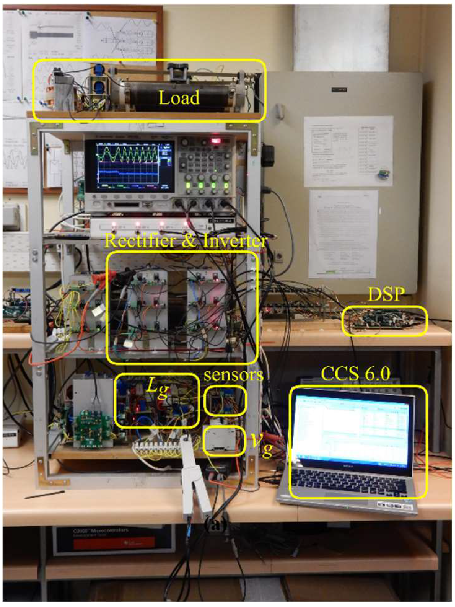
6. Experimental Results

In order to corroborate the theoretical and simulated results, a proof-of-concept prototype of the power converter shown in Figure 1 is implemented. The dynamic decoupling control algorithm was programmed in a TMS320F28335 DSP-based board. The complete experimental setup is presented in Figure 9.

Naturally, all the changes in real applications are smooth or ramp-type with a given duration. However, the mainly employed input for control purposes is the step, because it makes it possible to find several important parameters in the response of linear systems as overshoot, settling band and time. In this context, a step in the frequency is performed from 50 Hz to 100 Hz, which can be seen in Figure 10a. Although this process is nonlinear and despite the huge frequency change, it can be seen in Figure 10a that the control remains stable and after coupler cycles, the power factor becomes unitary and the dc voltage returns to its previous value, even though the dc voltage is affected only a little. To complement the tests, Figure 10b shows a ramp-up frequency sweep, where in this case, the power factor and the voltage remain very close to their references and no ramble can be perceived, displaying the good performance under frequency variation of the dynamic decoupler.

A dc voltage step-up change is performed and depicted in Figure 10c,d for f_g = 50 and 100 (Hz), respectively. As can be seen, the dynamic decoupler-based controller is capable of working in this wide variation frequency, as expected and theoretically demonstrated by the stability analysis. On the other hand, both responses look to be similar, even when the frequency—and, as a consequence, the impedance—changes by 100%.

The power factor response is tested and the results are presented in Figure 10e,f. The power factor goes from fp = 0.8 inductive to fp = 0.8 capacitive. The results show a similar behavior for f_g =50 Hz in Figure 10e and when f_g = 100 (Hz) in Figure 10f, even the wide frequency range tested. As stated previously for the dc voltage control, the frequency does not affect much in the dynamic behavior, and again, the control remains stable, as expected and demonstrated mathematically.

Since the tests using the static decoupler are destructive, as presented in Figure 7, the simulations performed in the previous section are used as a basis for comparison, which show instabilities below the 80 Hz, Table 2. Although the dynamic decoupler has a better behavior, its computation effort is greater than the static decoupler, and a dedicated digital board is required. Nevertheless, it is important to highlight that the computing time is similar for both cases because most of the time is required for the sensed variables acquisition, PI controllers, PLLs and the rest of the DSP related functions.

7. Discussion

The behavior of two dq SRF based control schemes based on static and dynamic decouplers has been studied and tested in the presence of wide frequency variations. The theoretical and simulation results show that under frequency variations, the system could reach instability depending upon the chosen control approach, particularly in the case when a static decoupler is considered, which is the most simple and common approach. Although the controller based on this approach remains stable up to 80 Hz for the used parameter set, oscillations with big excursions are obtained. Additionally, if the system’s parameters vary; for instance, the filter inductor, the stability region for the frequency can be substantially reduced, leading to a 25% reduction for a 30% increase in the inductor value. On the other hand, the dynamic decoupler-based controller shows a larger stability region than the static one. Indeed, an increase of up to 100% in the frequency does not induce instability. It can be concluded from the results that from the control point of view, although dynamic decouplers are computationally heavier, in some cases they are required to ensure proper behavior. A comparison of key characteristics of both approaches is summarized in

Table 3. Comparison of key features of static and dynamic decoupler based controllers.

Controller Algorithm	Robustness to Frequency Variation	Computational Burden	Dynamic Performance	Maintains Tuned Characteristics	Uses Frequency Value
Static decoupler based	Med	Low	Low	No	No
Dynamic decoupler based	High	Med	High	Yes	Yes

.

The proposed procedure based on Lyapunov criteria can be extended to any other grid—connected power converter configuration—as a current source or voltage source converters in order to verify the closed loop system’s stability. Furthermore, this study can be extended to any dynamic decoupler [34,36,38] and static decoupler [33]-based controller, and topologies with LCL filters where four new state variables would be added (6). The procedure can be summarized as follows:

• ➢ Define the model in the variable state representation;
• ➢ Define the controllers in the variable state representation;
• ➢ Build the representation of the whole system, including all the dynamics in the power converters, as currents, voltages, PLL internal dynamics, controllers, etc.;
• ➢ Determine the Jacobian as a function of the rest of the variables;
• ➢ Find the eigenvalues as a function of the variables of interest such as frequency, parameters and operating points where the system would work.

The aforementioned procedure can give useful guidelines, making it possible to characterize the operation of power converters controllers under frequency variations.

8. Conclusions

This work has comprehensively analyzed the stability characteristics and behavior of SRF-based linear-based controllers as used in grid-connected three-phase power converters when they are connected to a variable supply frequency environment. These converters, which are used as key building blocks of renewable energy interfaces and motor drives, are likely to operate under these conditions if used in micro and weak grids, where important frequency variations are expected. The theoretical analysis based on the Lyapunov indirect method has considered a static decoupler-based SRF controller, which effectively considers the system’s frequency a constant parameter, the most common approach, and a dynamic decoupler based one, where the true system’s frequency, estimated by a PLL, is used by the controller.

In the first case, when a static decoupler is considered, it has been found from the study of the eigenvalues of a representative system that instabilities do not appear in power systems with normal frequency variations (8 Hz range), although a poor dynamic behavior is obtained. Nevertheless, the results show that wide frequency variations lead to control system instability if the frequency is sufficiently increased. Indeed, for the parameters set under study, the critical frequency results were equal to 81.7 Hz. Furthermore, if an error exists in the parameters of the system, the critical frequency is further lowered. For instance, if the filter inductor is increased to 130%, the critical frequency is reduced to 62.4 Hz, i.e., only a 12.4 Hz tolerance. In other words, a static decoupler shows a limited stable operating region when frequency variations are expected.

On the other hand, the dynamic decoupler-based controller uses the frequency information from the PLL to increase the allowable frequency operating range. The results show that for our system under study, the ac mains frequency may even go twice the nominal one (from 50 Hz up to 100 Hz), while the system remains stable. Thus, the frequency operating region is substantially increased, which is a key advantage over the static decoupler for these power systems. From the presented results, it can be concluded that power converters controllers must be carefully designed when supply frequency variations are expected, taking into account the expected variations in the grid frequency, as has been shown. To this end, the presented methodology can be a useful tool for the evaluation of the controller’s behavior.

References

1. Young, K.; Dougal, R.A. SRF-PLL with Dynamic Center Frequency for Improved Phase Detection. In Proceedings of the 2009 International Conference on Clean Electrical Power, Capri, Italy, 9–11 June 2009; pp. 212–216. [Google Scholar]
2. Zhang, Z.; Liu, Y.; Li, J. A HESM-Based Variable Frequency AC Starter-Generator System for Aircraft Applications. IEEE Trans. Energy Convers. 2018, 33, 1998–2006. [Google Scholar] [CrossRef]
3. Zanchetta, P.; Degano, M.; Liu, J.; Mattavelli, P. Iterative Learning Control With Variable Sampling Frequency for Current Control of Grid-Connected Converters in Aircraft Power Systems. IEEE Trans. Ind. Appl. 2013, 49, 1548–1555. [Google Scholar] [CrossRef]
4. Rohten, J.A.; Espinoza, J.R.; Munoz, J.A.; Sbarbaro, D.G.; Perez, M.A.; Melin, P.E.; Silva, J.J.; Espinosa, E.E. Enhanced Predictive Control for a Wide Time-Variant Frequency Environment. IEEE Trans. Ind. Electron. 2016, 63, 5827–5837. [Google Scholar] [CrossRef]
5. Rohten, J.A.; Silva, J.J.; Munoz, J.A.; Villarroel, F.A.; Dewar, D.N.; Rivera, M.E.; Espinoza, J.R. A Simple Self-Tuning Resonant Control Approach for Power Converters Connected to Micro-Grids With Distorted Voltage Conditions. IEEE Access 2020, 8, 216018–216028. [Google Scholar] [CrossRef]
6. Ntomalis, S.; Iliadis, P.; Atsonios, K.; Nesiadis, A.; Nikolopoulos, N.; Grammelis, P. Dynamic Modeling and Simulation of Non-Interconnected Systems under High-RES Penetration: The Madeira Island Case. Energies 2020, 13, 5786. [Google Scholar] [CrossRef]
7. Azizipanah-Abarghooee, R.; Malekpour, M.; Dragicevic, T.; Blaabjerg, F.; Terzija, V. A Linear Inertial Response Emulation for Variable Speed Wind Turbines. IEEE Trans. Power Syst. 2020, 35, 1198–1208. [Google Scholar] [CrossRef]
8. Areerak, K.-N.; Wu, T.; Bozhko, S.V.; Asher, G.M.; Thomas, D.W.P. Aircraft Power System Stability Study Including Effect of Voltage Control and Actuators Dynamic. IEEE Trans. Aerosp. Electron. Syst. 2011, 47, 2574–2589. [Google Scholar] [CrossRef]
9. Etxegarai, A.; Eguia, P.; Torres, E.; Iturregi, A.; Valverde, V. Review of Grid Connection Requirements for Generation Assets in Weak Power Grids. Renew. Sustain. Energy Rev. 2015, 41, 1501–1514. [Google Scholar] [CrossRef]
10. Luo, X.; Wang, J.; Wojcik, J.; Wang, J.; Li, D.; Draganescu, M.; Li, Y.; Miao, S. Review of Voltage and Frequency Grid Code Specifications for Electrical Energy Storage Applications. Energies 2018, 11, 1070. [Google Scholar] [CrossRef]
11. Herrejón-Pintor, G.A.; Melgoza-Vázquez, E.; Chávez, J.D.J. A Modified SOGI-PLL with Adjustable Refiltering for Improved Stability and Reduced Response Time. Energies 2022, 15, 4253. [Google Scholar] [CrossRef]
12. Aldbaiat, B.; Nour, M.; Radwan, E.; Awada, E. Grid-Connected PV System with Reactive Power Management and an Optimized SRF-PLL Using Genetic Algorithm. Energies 2022, 15, 2177. [Google Scholar] [CrossRef]
13. Liu, B.; An, M.; Wang, H.; Chen, Y.; Zhang, Z.; Xu, C.; Song, S.; Lv, Z. A Simple Approach to Reject DC Offset for Single-Phase Synchronous Reference Frame PLL in Grid-Tied Converters. IEEE Access 2020, 8, 112297–112308. [Google Scholar] [CrossRef]
14. Huang, Y.; Wang, D. Effect of Control-Loops Interactions on Power Stability Limits of VSC Integrated to AC System. IEEE Trans. Power Deliv. 2018, 33, 301–310. [Google Scholar] [CrossRef]
15. Liu, R.; Wang, S.; Liu, G.; Wen, S.; Zhang, J.; Ma, Y. An Improved Virtual Inertia Control Strategy for Low Voltage AC Microgrids with Hybrid Energy Storage Systems. Energies 2022, 15, 442. [Google Scholar] [CrossRef]
16. Bimarta, R.; Tran, T.V.; Kim, K.-H. Frequency-Adaptive Current Controller Design Based on LQR State Feedback Control for a Grid-Connected Inverter under Distorted Grid. Energies 2018, 11, 2674. [Google Scholar] [CrossRef]
17. Panda, R.K.; Mohapatra, A.; Srivastava, S.C. Enhancing Inertia of Solar Photovoltaic-based Microgrid through Notch Filter-based PLL in SRF Control. IET Gener. Transm. Distrib. 2020, 14, 379–388. [Google Scholar] [CrossRef]
18. Xia, T.; Zhang, X.; Tan, G.; Liu, Y. All-Pass-Filter-Based PLL for Single-Phase Grid-Connected Converters Under Distorted Grid Conditions. IEEE Access 2020, 8, 106226–106233. [Google Scholar] [CrossRef]
19. Xu, J.; Qian, Q.; Zhang, B.; Xie, S. Harmonics and Stability Analysis of Single-Phase Grid-Connected Inverters in Distributed Power Generation Systems Considering Phase-Locked Loop Impact. IEEE Trans. Sustain. Energy 2019, 10, 1470–1480. [Google Scholar] [CrossRef]
20. Luo, W.; Wei, D. A Frequency-Adaptive Improved Moving-Average-Filter-Based Quasi-Type-1 PLL for Adverse Grid Conditions. IEEE Access 2020, 8, 54145–54153. [Google Scholar] [CrossRef]
21. Yogarathinam, A.; Kaur, J.; Chaudhuri, N.R. Impact of Inertia and Effective Short Circuit Ratio on Control of Frequency in Weak Grids Interfacing LCC-HVDC and DFIG-Based Wind Farms. IEEE Trans. Power Deliv. 2017, 32, 2040–2051. [Google Scholar] [CrossRef]
22. Rohten, J.A.; Espinoza, J.R.; Munoz, J.A.; Perez, M.A.; Melin, P.E.; Silva, J.J.; Espinosa, E.E.; Rivera, M.E. Model Predictive Control for Power Converters in a Distorted Three-Phase Power Supply. IEEE Trans. Ind. Electron. 2016, 63, 5838–5848. [Google Scholar] [CrossRef]
23. Zuniga-Reyes, M.-A.; Robles-Ocampo, J.-B.; Sevilla-Camacho, P.-Y.; Rodriguez-Resendiz, J.; Lastres-Danguillecourt, O.; Conde-Diaz, J.-E. Photovoltaic Failure Detection Based on String-Inverter Voltage and Current Signals. IEEE Access 2021, 9, 39939–39954. [Google Scholar] [CrossRef]
24. Estévez-Bén, A.A.; Alvarez-Diazcomas, A.; Rodríguez-Reséndiz, J. Transformerless Multilevel Voltage-Source Inverter Topology Comparative Study for PV Systems. Energies 2020, 13, 3261. [Google Scholar] [CrossRef]
25. Estévez-Bén, A.A.; Alvarez-Diazcomas, A.; Macias-Bobadilla, G.; Rodríguez-Reséndiz, J. Leakage Current Reduction in Single-Phase Grid-Connected Inverters—A Review. Appl. Sci. 2020, 10, 2384. [Google Scholar] [CrossRef]
26. Alvarez-Diazcomas, A.; López, H.; Carrillo-Serrano, R.V.; Rodríguez-Reséndiz, J.; Vázquez, N.; Herrera-Ruiz, G. A Novel Integrated Topology to Interface Electric Vehicles and Renewable Energies with the Grid. Energies 2019, 12, 4091. [Google Scholar] [CrossRef]
27. Estévez-Bén, A.A.; López Tapia, H.J.C.; Carrillo-Serrano, R.V.; Rodríguez-Reséndiz, J.; Vázquez Nava, N. A New Predictive Control Strategy for Multilevel Current-Source Inverter Grid-Connected. Electronics 2019, 8, 902. [Google Scholar] [CrossRef]
28. Lopez, H.; Rodriguez Resendiz, J.; Guo, X.; Vazquez, N.; Carrillo-Serrano, R.V. Transformerless Common-Mode Current-Source Inverter Grid-Connected for PV Applications. IEEE Access 2018, 6, 62944–62953. [Google Scholar] [CrossRef]
29. Zhang, X.; Chen, Y.; Wang, Y.; Zha, X.; Yue, S.; Cheng, X.; Gao, L. Deloading Power Coordinated Distribution Method for Frequency Regulation by Wind Farms Considering Wind Speed Differences. IEEE Access 2019, 7, 122573–122582. [Google Scholar] [CrossRef]
30. Mujcinagic, A.; Kusljugic, M.; Nukic, E. Wind Inertial Response Based on the Center of Inertia Frequency of a Control Area. Energies 2020, 13, 6177. [Google Scholar] [CrossRef]
31. Li, T.; Li, Y.; Yang, J.; Ge, W.; Hu, B. A Modified DSC-Based Grid Synchronization Method for a High Renewable Penetrated Power System Under Distorted Voltage Conditions. Energies 2019, 12, 4040. [Google Scholar] [CrossRef] [Green Version]
32. Wang, M.; Wang, X.; Qiao, J.; Wang, L. Improved Current Decoupling Method for Robustness Improvement of LCL-Type STATCOM Based on Active Disturbance Rejection Control. IEEE Access 2019, 7, 121781–121792. [Google Scholar] [CrossRef]
33. Munoz, J.A.; Espinoza, J.R.; Moran, L.A.; Baier, C.R. Design of a Modular UPQC Configuration Integrating a Components Economical Analysis. IEEE Trans. Power Deliv. 2009, 24, 1763–1772. [Google Scholar] [CrossRef]
34. Rohten, J.A.; Espinoza, J.R.; Munoz, J.A.; Melin, P.E.; Espinosa, E.E. Discrete Nonlinear Control Based on a Double Dq Transform of a Multi-Cell UPQC. In Proceedings of the IECON 2011—37th Annual Conference of the IEEE Industrial Electronics Society, Melbourne, VIC, Australia, 7–10 November 2011; pp. 4134–4139. [Google Scholar]
35. Housseini, B.; Okou, A.F.; Beguenane, R. Robust Nonlinear Controller Design for On-Grid/Off-Grid Wind Energy Battery-Storage System. IEEE Trans. Smart Grid 2018, 9, 5588–5598. [Google Scholar] [CrossRef]
36. Aliaga, R.; Rivera, M.; Wheeler, P.; Munoz, J.; Rohten, J.; Sebaaly, F.; Villalon, A.; Trentin, A. Implementation of Exact Linearization Technique for Modeling and Control of DC/DC Converters in Rural PV Microgrid Application. IEEE Access 2022, 10, 56925–56936. [Google Scholar] [CrossRef]
37. Ma, W.; Ouyang, S.; Zhang, J.; Xu, W. Control Strategy Based on $\text{H}\infty$ Repetitive Controller With Active Damping for Islanded Microgrid. IEEE Access 2019, 7, 162157–162168. [Google Scholar] [CrossRef]
38. Rohten, J.; Espinoza, J.; Villarroel, F.; Perez, M.; Munoz, J.; Melin, P.; Espinosa, E. Static Power Converter Synchronization and Control under Varying Frequency Conditions. In Proceedings of the IECON 2012—38th Annual Conference on IEEE Industrial Electronics Society, Montreal, QC, Canada, 25–28 October 2012; pp. 786–791. [Google Scholar]
39. Munoz, J.; Baier, C.; Espinoza, J.; Rivera, M.; Guzman, J.; Rohten, J. Switching Losses Analysis of an Asymmetric Multilevel Shunt Active Power Filter. In Proceedings of the IECON 2013—39th Annual Conference of the IEEE Industrial Electronics Society, Vienna, Austria, 10–13 November 2013; pp. 8534–8539. [Google Scholar]
40. Munoz, J.A.; Reyes, J.R.; Espinoza, J.R.; Rubilar, I.A.; Moran, L.A. A Novel Multi-Level Three-Phase UPQC Topology Based on Full-Bridge Single-Phase Cells. In Proceedings of the IECON 2007—33rd Annual Conference of the IEEE Industrial Electronics Society, Taipei, Taiwan, 5–8 November 2007; pp. 1787–1792. [Google Scholar]
41. Dewar, D.; Rohten, J.; Formentini, A.; Zanchetta, P. Decentralised Optimal Controller Design of Variable Frequency Three-Phase Power Electronic Networks Accounting for Sub-System Interactions. IEEE Open J. Ind. Appl. 2020, 1, 270–282. [Google Scholar] [CrossRef]
Figure 1. Power Converter System.
Sensors 22 07078 g001
Figure 2. Power converter rectifier with a static decoupler control.
Sensors 22 07078 g002
Figure 3. Power converter rectifier with a dynamic decoupler control.
Sensors 22 07078 g003
Figure 4. AL eigenvalues as a function of the ac main frequency (from 30 to 100 Hz); (a) all six values; (b) zoom to the unstable eigenvalues.
Sensors 22 07078 g004
Figure 5. The imaginary closest eigenvalue evolution as a function of parameters with frequency (from 30 to 100 Hz). (a) Lg from 70% to 130% with respect the nominal value; (b) Rg from 70% to 130% with respect the nominal value; (c) Cdc from 70% to 130% with respect the nominal value.
Sensors 22 07078 g005
Figure 6. ANL eigenvalues as a function of the ac main frequency (from 30 to 100 Hz), (a) all six values, (b) zoom to the unstable eigenvalues.
Sensors 22 07078 g006
Figure 7. Linear control response; (a) synchronization; (b) dc voltage; (c) power factor; (d) input rectifier currents.
Sensors 22 07078 g007
Figure 8. Nonlinear control response; (a) synchronization; (b) dc voltage; (c) power factor; (d) input rectifier currents.
Sensors 22 07078 g008
Figure 9. Experimental three-phase grid-connected power converter system.
Sensors 22 07078 g009
Figure 10. Results for dynamic decoupler; (a) step-up frequency change; (b) ramp-up frequency change; (c) dc voltage step-up response with fg = 50 Hz; (d) dc voltage step-up response with fg = 100 Hz; (e) power factor step response with fg = 50 Hz; (f) power factor step response with fg = 100 Hz.
Sensors 22 07078 g010