

A Comprehensive Survey of Depth Completion Approaches

 , , ,
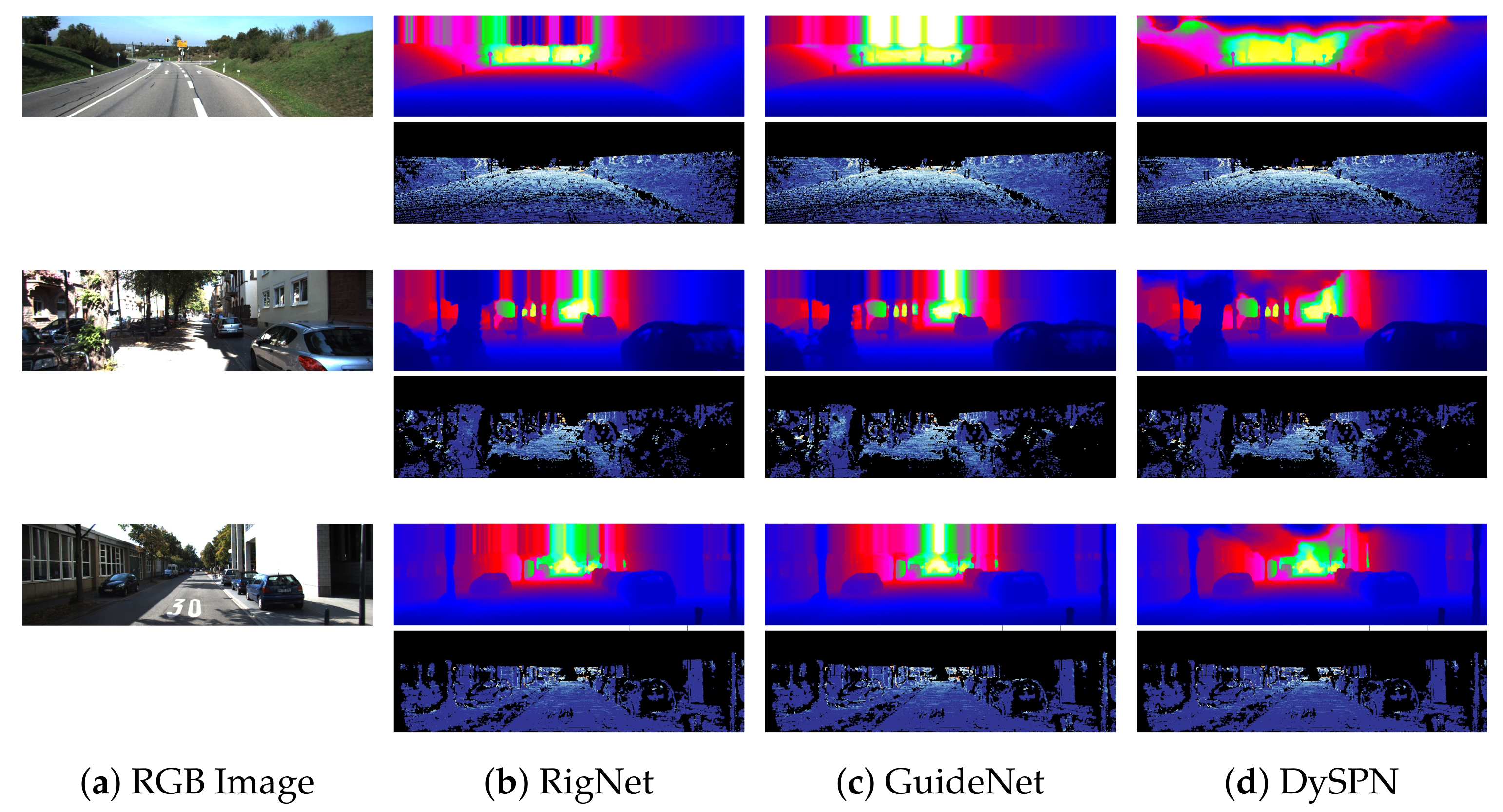
, , ,  ,
, 
Abstract
:1. Introduction
2. Methodologies
2.1. Unguided Methods
2.2. Image-Guided Methods
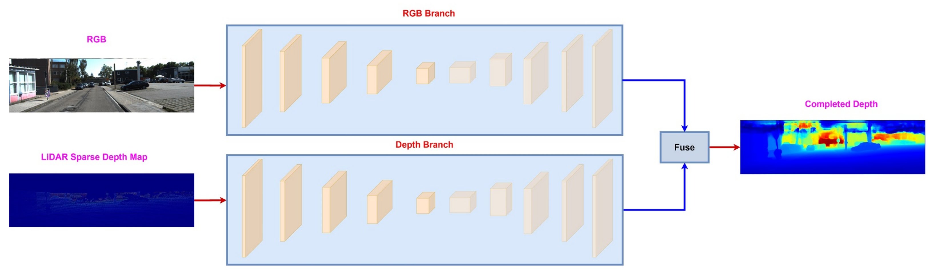
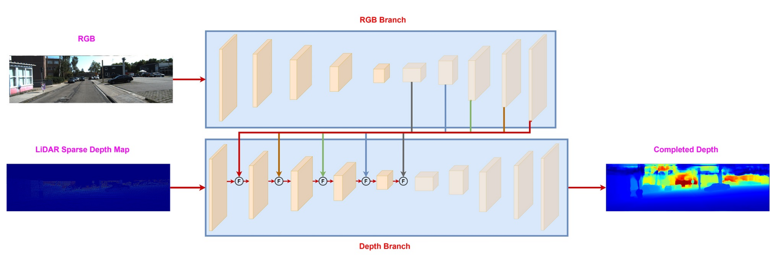
2.2.1. Multi-Branch Networks
Guided Image Filtering
2.2.2. Spatial Propagation Networks (SPN)
3. Multi-Modal Fusion
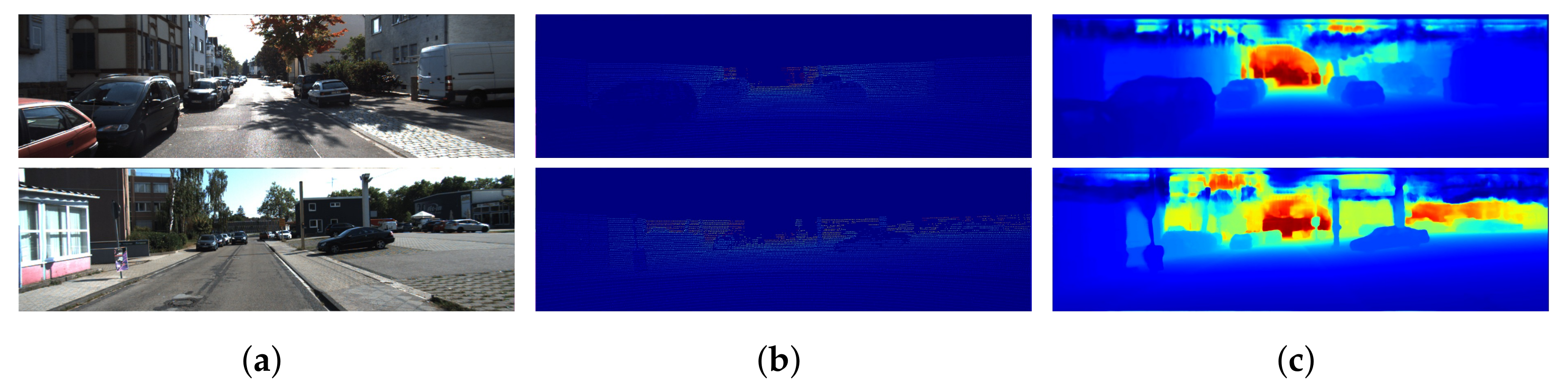
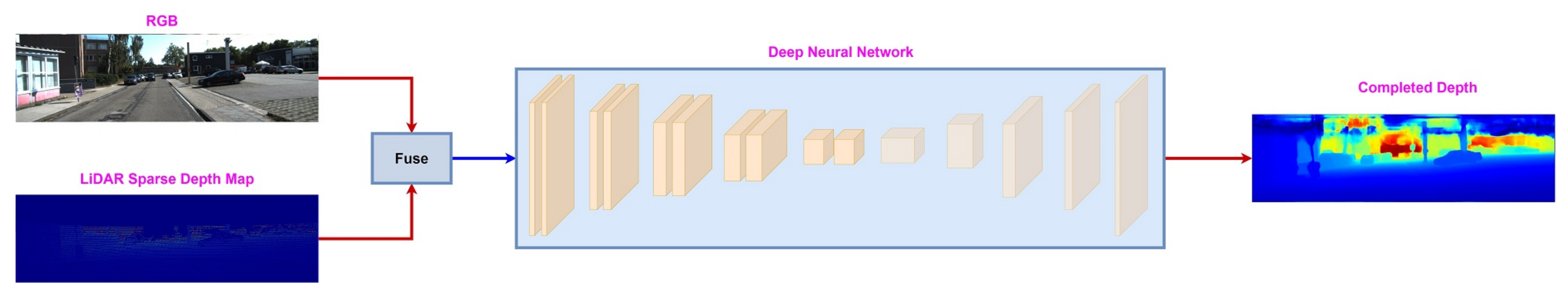
3.1. Early Fusion
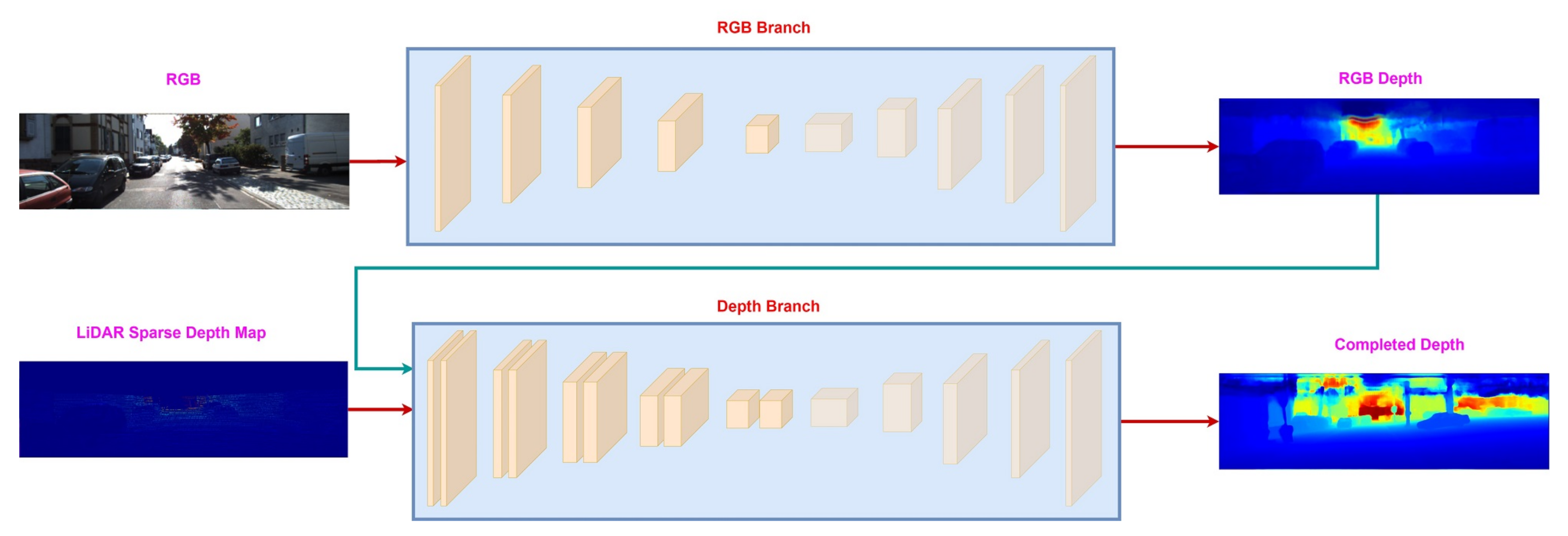
3.2. Sequential Fusion

| Strategy | Key Idea | Advantages | Disadvantages |
|---|---|---|---|
| Early [20,22,23,32,33,35,48] | Creation of a unified representation of related input modalities e.g., RGB images and LiDAR sparse depth maps. The joint representation is passed as an input to a neural network for joint processing. |
|
|
| Sequential [30,32,35] | It is a multi-stage approach. The aim of the first stage is to focus on a single modality e.g., RGB image, and produce an intermediate output e.g., color depth, whereas, in the second stage, unimodal information including LiDAR sparse depth and color depth are combined to generate the final dense map. |
|
|
| Late [17,32,35,48,51,64] | The idea is to process unimodal information (RGB, LiDAR) separately and then create a unified representation at the output level. |
|
|
| Deep [33,35,48,51] | Performs fusion at intermediate (feature) level between the unimodal branches((RGB, LiDAR). |
|
|
3.3. Late Fusion
3.4. Deep Fusion
4. Datasets
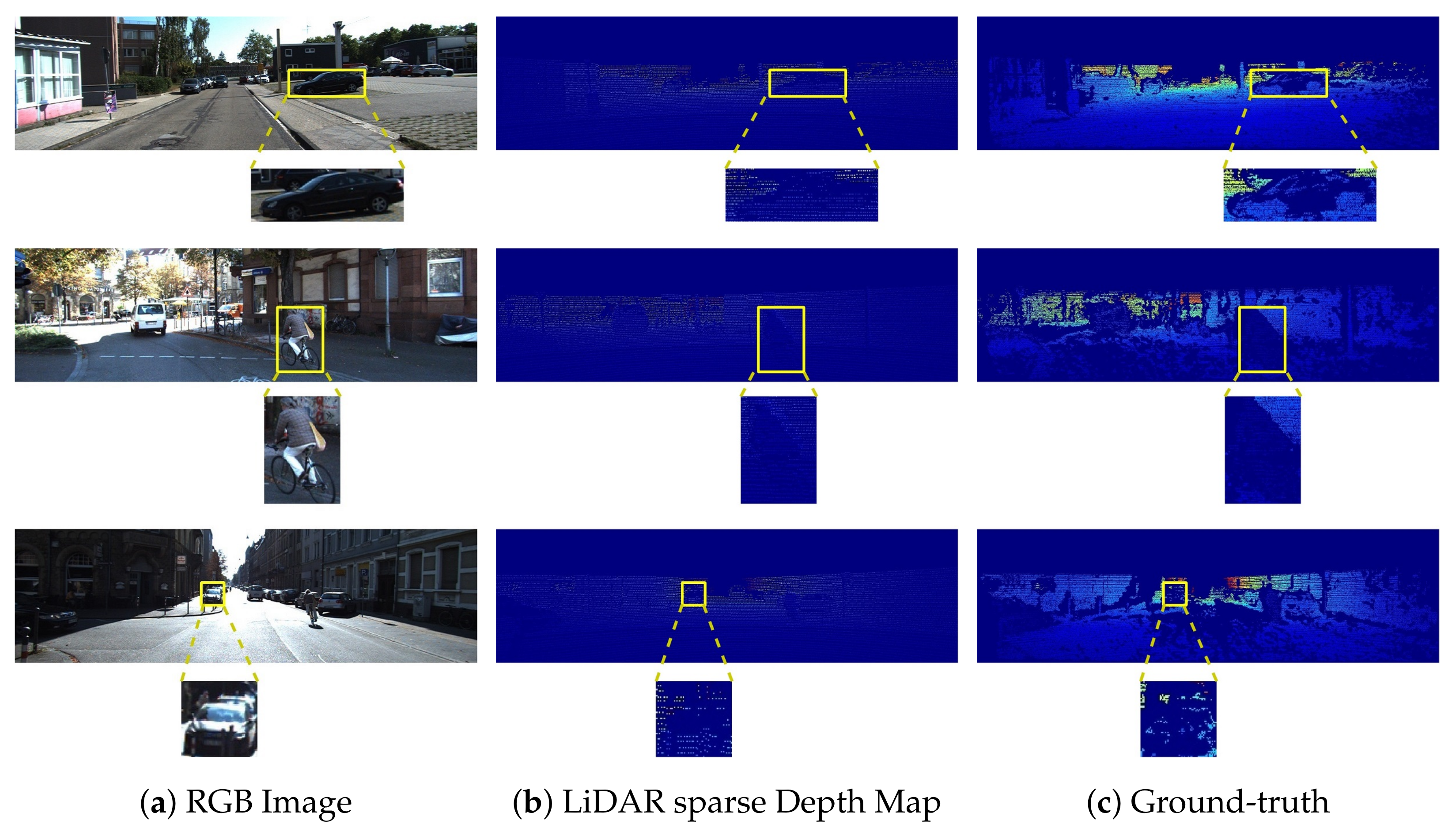
4.1. KITTI Dataset
KITTI Depth Completion Benchmark
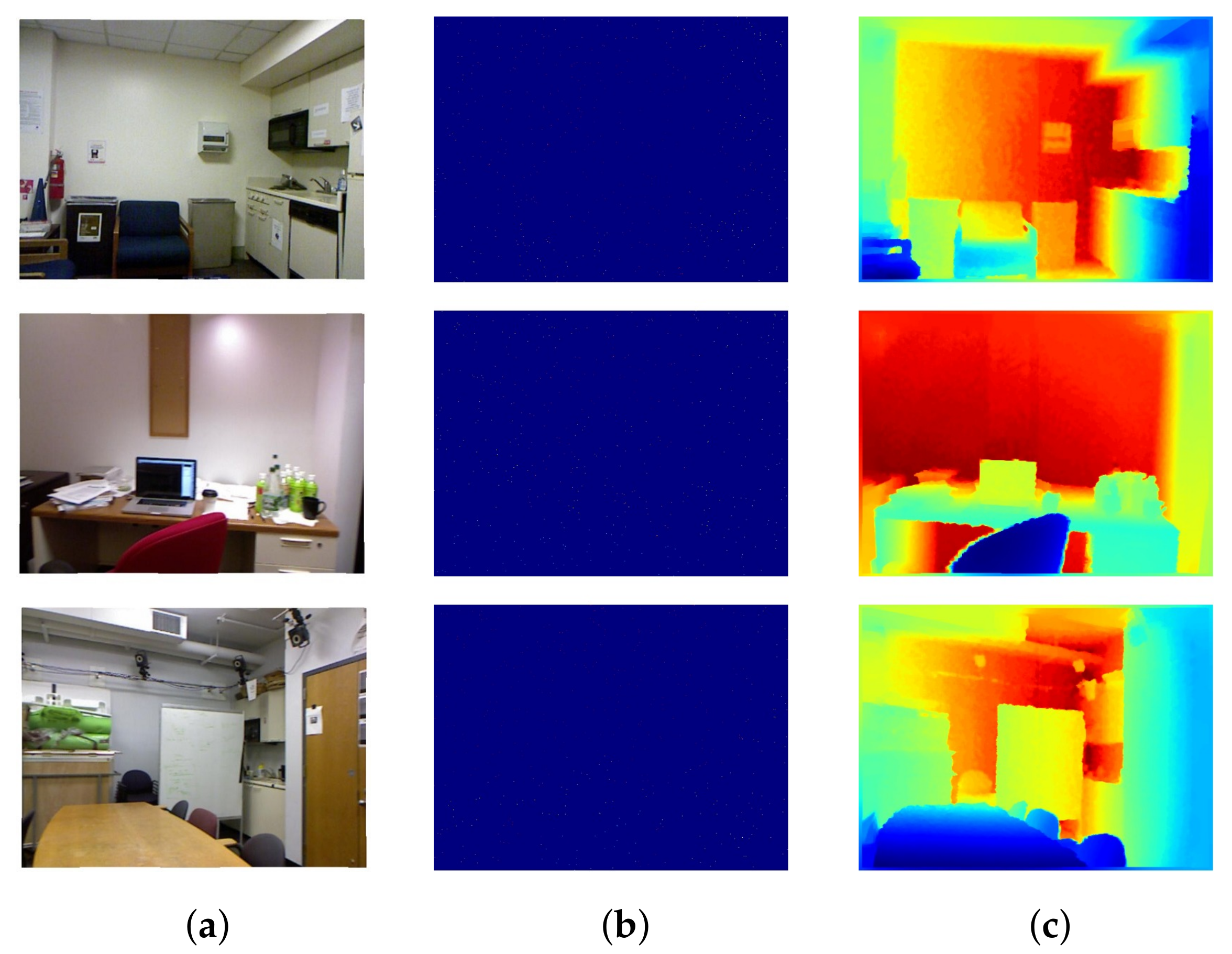
4.2. Nyu-v2 Depth Dataset
5. Evaluation Metrics
6. Objective Functions
6.1. Supervised Learning
6.2. Unsupervised Learning
7. Results
| Category | Method | RMSE | MAE | iRMSE | iMAE |
|---|---|---|---|---|---|
| Multi-branch Networks | SSGP [47] | 838.00 | 245.00 | - | - |
| DDP [39] | 836.00 | 205.40 | 2.12 | 0.86 | |
| MS-Net[LF]-L2 [19] | 829.98 | 233.26 | 2.60 | 1.03 | |
| S2D [15] | 814.73 | 249.95 | 2.81 | 1.21 | |
| CrossGuidance [44] | 807.42 | 253.98 | 2.73 | 1.33 | |
| RSIC [46] | 792.80 | 225.81 | 2.42 | 0.99 | |
| Depth-normal [38] | 777.05 | 235.17 | 2.42 | 1.13 | |
| FusionNet [23] | 772.87 | 215.02 | 2.19 | 0.93 | |
| MSG-CHN [41] | 762.19 | 220.41 | 2.30 | 0.98 | |
| DeepLiDAR [20] | 758.38 | 226.50 | 2.56 | 1.15 | |
| DenseLiDAR [43] | 755.41 | 214.13 | 2.25 | 0.96 | |
| ACMNet [40] | 744.91 | 206.09 | 2.08 | 0.90 | |
| FCFR-Net [48] | 735.81 | 217.15 | 2.20 | 0.98 | |
| PENet [32] | 730.08 | 210.55 | 2.17 | 0.94 | |
| RigNet [33] | 712.66 | 203.25 | 2.08 | 0.90 | |
| Guided Image Filtering | GuideNet [51] | 739.24 | 218.83 | 2.25 | 0.99 |
| Spatial Propagation Networks | CSPN [21] | 1019.64 | 279.46 | 2.93 | 1.15 |
| DSPN [59] | 766.74 | 220.36 | 2.47 | 1.03 | |
| CSPN++ [22] | 743.69 | 209.28 | 2.07 | 0.90 | |
| NLSPN [11] | 741.68 | 199.59 | 1.99 | 0.84 | |
| DySPN [60] | 709.12 | 192.71 | 1.88 | 0.82 |
| Category | Method | RMSE | REL | |||
|---|---|---|---|---|---|---|
| Multi-Branch Networks | S2D [15] | 0.133 | 0.027 | - | - | - |
| EncDec-Net[EF] [19] | 0.123 | 0.017 | 99.1 | 99.8 | 100 | |
| DeepLiDAR [20] | 0.115 | 0.022 | 99.3 | 99.9 | 100.0 | |
| Xu et. al. [38] | 0.112 | 0.018 | 99.5 | 99.9 | 100.0 | |
| FCFR-Net [48] | 0.106 | 0.015 | 99.5 | 99.9 | 100.0 | |
| ACMNet [40] | 0.105 | 0.015 | 99.4 | 99.9 | 100 | |
| DenseLiDAR [43] | 0.105 | 0.015 | 99.4 | 99.9 | 100 | |
| RigNet [33] | 0.090 | 0.013 | 99.6 | 99.9 | 100.0 | |
| Guided Image Filtering | GuideNet [51] | 0.101 | 0.015 | 99.5 | 99.9 | 100.0 |
| Spatial Propagation Networks | CSPN [21] | 0.117 | 0.016 | 99.2 | 99.9 | 100.0 |
| CSPN++ [22] | 0.116 | - | - | - | - | |
| NLSPN [11] | 0.092 | 0.012 | 99.6 | 99.9 | 100.0 | |
| DySPN [60] | 0.091 | 0.012 | 99.6 | 99.9 | 100.0 |
8. Conclusions
Author Contributions
Funding
Institutional Review Board Statement
Informed Consent Statement
Data Availability Statement
Conflicts of Interest
References
- Cui, Z.; Heng, L.; Yeo, Y.C.; Geiger, A.; Pollefeys, M.; Sattler, T. Real-time dense mapping for self-driving vehicles using fisheye cameras. In Proceedings of the 2019 International Conference on Robotics and Automation (ICRA), Montreal, QC, Canada, 20–24 May 2019; pp. 6087–6093. [Google Scholar]
- Häne, C.; Heng, L.; Lee, G.H.; Fraundorfer, F.; Furgale, P.; Sattler, T.; Pollefeys, M. 3D visual perception for self-driving cars using a multi-camera system: Calibration, mapping, localization, and obstacle detection. Image Vis. Comput. 2017, 68, 14–27. [Google Scholar] [CrossRef]
- Wang, K.; Zhang, Z.; Yan, Z.; Li, X.; Xu, B.; Li, J.; Yang, J. Regularizing Nighttime Weirdness: Efficient Self-supervised Monocular Depth Estimation in the Dark. In Proceedings of the IEEE/CVF International Conference on Computer Vision, Virtual, 11–17 October 2021; pp. 16055–16064. [Google Scholar]
- Song, X.; Wang, P.; Zhou, D.; Zhu, R.; Guan, C.; Dai, Y.; Su, H.; Li, H.; Yang, R. Apollocar3d: A large 3d car instance understanding benchmark for autonomous driving. In Proceedings of the IEEE/CVF Conference on Computer Vision and Pattern Recognition, Long Beach, CA, USA, 16–17 June 2019; pp. 5452–5462. [Google Scholar]
- Liao, Y.; Huang, L.; Wang, Y.; Kodagoda, S.; Yu, Y.; Liu, Y. Parse geometry from a line: Monocular depth estimation with partial laser observation. In Proceedings of the 2017 IEEE International Conference on Robotics and Automation (ICRA), Singapore, 29 May–3 June 2017; pp. 5059–5066. [Google Scholar]
- Dey, A.; Jarvis, G.; Sandor, C.; Reitmayr, G. Tablet versus phone: Depth perception in handheld augmented reality. In Proceedings of the 2012 IEEE international symposium on mixed and augmented reality (ISMAR), Atlanta, GA, USA, 5–8 November 2012; pp. 187–196. [Google Scholar]
- Kalia, M.; Navab, N.; Salcudean, T. A Real-Time Interactive Augmented Reality Depth Estimation Technique for Surgical Robotics. In Proceedings of the 2019 International Conference on Robotics and Automation (ICRA), Montreal, QC, Canada, 20–24 May 2019; pp. 8291–8297. [Google Scholar] [CrossRef]
- Holynski, A.; Kopf, J. Fast depth densification for occlusion-aware augmented reality. ACM Trans. Graph. (ToG) 2018, 37, 1–11. [Google Scholar] [CrossRef]
- Armbrüster, C.; Wolter, M.; Kuhlen, T.; Spijkers, W.; Fimm, B. Depth perception in virtual reality: Distance estimations in peri-and extrapersonal space. Cyberpsychol. Behav. 2008, 11, 9–15. [Google Scholar] [CrossRef] [PubMed]
- Huang, H.C.; Hsieh, C.T.; Yeh, C.H. An Indoor Obstacle Detection System Using Depth Information and Region Growth. Sensors 2015, 15, 27116–27141. [Google Scholar] [CrossRef] [PubMed]
- Park, J.; Joo, K.; Hu, Z.; Liu, C.K.; So Kweon, I. Non-local spatial propagation network for depth completion. In Proceedings of the European Conference on Computer Vision, Glasgow, UK, 23–28 August 2020; Springer: Berlin/Heidelberg, Germany, 2020; pp. 120–136. [Google Scholar]
- Nguyen, T.N.; Huynh, H.H.; Meunier, J. 3D Reconstruction With Time-of-Flight Depth Camera and Multiple Mirrors. IEEE Access 2018, 6, 38106–38114. [Google Scholar] [CrossRef]
- Zhang, Z.; Cui, Z.; Xu, C.; Yan, Y.; Sebe, N.; Yang, J. Pattern-affinitive propagation across depth, surface normal and semantic segmentation. In Proceedings of the IEEE/CVF Conference on Computer Vision and Pattern Recognition, Long Beach, CA, USA, 15–20 June 2019; pp. 4106–4115. [Google Scholar]
- Wang, Y.; Chao, W.L.; Garg, D.; Hariharan, B.; Campbell, M.; Weinberger, K.Q. Pseudo-lidar from visual depth estimation: Bridging the gap in 3d object detection for autonomous driving. In Proceedings of the IEEE/CVF Conference on Computer Vision and Pattern Recognition, Long Beach, CA, USA, 15–20 June 2019; pp. 8445–8453. [Google Scholar]
- Ma, F.; Cavalheiro, G.V.; Karaman, S. Self-supervised sparse-to-dense: Self-supervised depth completion from lidar and monocular camera. In Proceedings of the 2019 International Conference on Robotics and Automation (ICRA), Montreal, QC, Canada, 20–24 May 2019; pp. 3288–3295. [Google Scholar]
- Chodosh, N.; Wang, C.; Lucey, S. Deep convolutional compressed sensing for lidar depth completion. In Proceedings of the Asian Conference on Computer Vision, Perth, Australia, 2–6 December 2018; Springer: Berlin/Heidelberg, Germany, 2018; pp. 499–513. [Google Scholar]
- Jaritz, M.; De Charette, R.; Wirbel, E.; Perrotton, X.; Nashashibi, F. Sparse and dense data with cnns: Depth completion and semantic segmentation. In Proceedings of the 2018 International Conference on 3D Vision (3DV), Verona, Italy, 5–8 September 2018; pp. 52–60. [Google Scholar]
- Uhrig, J.; Schneider, N.; Schneider, L.; Franke, U.; Brox, T.; Geiger, A. Sparsity invariant cnns. In Proceedings of the 2017 International Conference on 3D Vision (3DV), Qingdao, China, 10–12 October 2017; pp. 11–20. [Google Scholar]
- Eldesokey, A.; Felsberg, M.; Khan, F.S. Confidence propagation through cnns for guided sparse depth regression. IEEE Trans. Pattern Anal. Mach. Intell. 2019, 42, 2423–2436. [Google Scholar] [CrossRef]
- Qiu, J.; Cui, Z.; Zhang, Y.; Zhang, X.; Liu, S.; Zeng, B.; Pollefeys, M. Deeplidar: Deep surface normal guided depth prediction for outdoor scene from sparse lidar data and single color image. In Proceedings of the IEEE/CVF Conference on Computer Vision and Pattern Recognition, Long Beach, CA, USA, 15–20 June 2019; pp. 3313–3322. [Google Scholar]
- Cheng, X.; Wang, P.; Yang, R. Learning depth with convolutional spatial propagation network. IEEE Trans. Pattern Anal. Mach. Intell. 2019, 42, 2361–2379. [Google Scholar] [CrossRef]
- Cheng, X.; Wang, P.; Guan, C.; Yang, R. CSPN++: Learning Context and Resource Aware Convolutional Spatial Propagation Networks for Depth Completion. arXiv 2019, arXiv:1911.05377. [Google Scholar] [CrossRef]
- Van Gansbeke, W.; Neven, D.; De Brabandere, B.; Van Gool, L. Sparse and noisy lidar completion with rgb guidance and uncertainty. In Proceedings of the 2019 16th International Conference on Machine Vision Applications (MVA), Tokyo, Japan, 27–31 May 2019; pp. 1–6. [Google Scholar]
- Bertalmio, M.; Bertozzi, A.L.; Sapiro, G. Navier-stokes, fluid dynamics, and image and video inpainting. In Proceedings of the 2001 IEEE Computer Society Conference on Computer Vision and Pattern Recognition, Kauai, HI, USA, 8–14 December 2001; Volume 1, p. I. [Google Scholar]
- Herrera, D.; Kannala, J.; Ladický, L.; Heikkilä, J. Depth map inpainting under a second-order smoothness prior. In Proceedings of the Scandinavian Conference on Image Analysis, Espoo, Finland, 17–20 June 2013; Springer: Berlin/Heidelberg, Germany, 2013; pp. 555–566. [Google Scholar]
- Doria, D.; Radke, R.J. Filling large holes in lidar data by inpainting depth gradients. In Proceedings of the 2012 IEEE Computer Society Conference on Computer Vision and Pattern Recognition Workshops, Providence, RI, USA, 16–21 June 2012; pp. 65–72. [Google Scholar]
- Ferstl, D.; Reinbacher, C.; Ranftl, R.; Rüther, M.; Bischof, H. Image guided depth upsampling using anisotropic total generalized variation. In Proceedings of the IEEE International Conference on Computer Vision, Sydney, Australia, 1–8 December 2013; pp. 993–1000. [Google Scholar]
- Matsuo, K.; Aoki, Y. Depth image enhancement using local tangent plane approximations. In Proceedings of the IEEE Conference on Computer Vision and Pattern Recognition, Boston, MA, USA, 7–12 June 2015; pp. 3574–3583. [Google Scholar]
- Bai, L.; Zhao, Y.; Elhousni, M.; Huang, X. DepthNet: Real-Time LiDAR Point Cloud Depth Completion for Autonomous Vehicles. IEEE Access 2020, 8, 227825–227833. [Google Scholar] [CrossRef]
- Eldesokey, A.; Felsberg, M.; Holmquist, K.; Persson, M. Uncertainty-aware cnns for depth completion: Uncertainty from beginning to end. In Proceedings of the IEEE/CVF Conference on Computer Vision and Pattern Recognition, Seattle, WA, USA, 13–19 June 2020; pp. 12014–12023. [Google Scholar]
- Eldesokey, A.; Felsberg, M.; Khan, F.S. Propagating confidences through cnns for sparse data regression. arXiv 2018, arXiv:1805.11913. [Google Scholar]
- Hu, M.; Wang, S.; Li, B.; Ning, S.; Fan, L.; Gong, X. Penet: Towards precise and efficient image guided depth completion. In Proceedings of the 2021 IEEE International Conference on Robotics and Automation (ICRA), Xi’an, China, 30 May–5 June 2021; pp. 13656–13662. [Google Scholar]
- Yan, Z.; Wang, K.; Li, X.; Zhang, Z.; Xu, B.; Li, J.; Yang, J. RigNet: Repetitive image guided network for depth completion. arXiv 2021, arXiv:2107.13802. [Google Scholar]
- Zhang, C.; Tang, Y.; Zhao, C.; Sun, Q.; Ye, Z.; Kurths, J. Multitask GANs for Semantic Segmentation and Depth Completion With Cycle Consistency. IEEE Trans. Neural Netw. Learn. Syst. 2021, 32, 5404–5415. [Google Scholar] [CrossRef] [PubMed]
- Nazir, D.; Liwicki, M.; Stricker, D.; Afzal, M.Z. SemAttNet: Towards Attention-based Semantic Aware Guided Depth Completion. arXiv 2022, arXiv:2204.13635. [Google Scholar] [CrossRef]
- Zhang, Y.; Funkhouser, T. Deep depth completion of a single rgb-d image. In Proceedings of the IEEE Conference on Computer Vision and Pattern Recognition, Salt Lake City, UT, USA, 18–23 June 2018; pp. 175–185. [Google Scholar]
- Ronneberger, O.; Fischer, P.; Brox, T. U-net: Convolutional networks for biomedical image segmentation. In Proceedings of the International Conference on Medical Image Computing and Computer-Assisted Intervention, Munich, Germany, 5–9 October 2015; Springer: Berlin/Heidelberg, Germany, 2015; pp. 234–241. [Google Scholar]
- Xu, Y.; Zhu, X.; Shi, J.; Zhang, G.; Bao, H.; Li, H. Depth completion from sparse lidar data with depth-normal constraints. In Proceedings of the IEEE/CVF International Conference on Computer Vision, Seoul, Korea, 27–28 October 2019; pp. 2811–2820. [Google Scholar]
- Yang, Y.; Wong, A.; Soatto, S. Dense depth posterior (ddp) from single image and sparse range. In Proceedings of the IEEE/CVF Conference on Computer Vision and Pattern Recognition, Long Beach, CA, USA, 15–20 June 2019; pp. 3353–3362. [Google Scholar]
- Zhao, S.; Gong, M.; Fu, H.; Tao, D. Adaptive context-aware multi-modal network for depth completion. IEEE Trans. Image Process. 2021, 30, 5264–5276. [Google Scholar] [CrossRef] [PubMed]
- Li, A.; Yuan, Z.; Ling, Y.; Chi, W.; Zhang, C. A multi-scale guided cascade hourglass network for depth completion. In Proceedings of the IEEE/CVF Winter Conference on Applications of Computer Vision, Snowmass Village, CO, USA, 1–5 March 2020; pp. 32–40. [Google Scholar]
- Newell, A.; Yang, K.; Deng, J. Stacked hourglass networks for human pose estimation. In Proceedings of the European Conference on Computer Vision, Amsterdam, The Netherlands, 11–14 October 2016; Springer: Berlin/Heidelberg, Germany, 2016; pp. 483–499. [Google Scholar]
- Gu, J.; Xiang, Z.; Ye, Y.; Wang, L. DenseLiDAR: A real-time pseudo dense depth guided depth completion network. IEEE Robot. Autom. Lett. 2021, 6, 1808–1815. [Google Scholar] [CrossRef]
- Lee, S.; Lee, J.; Kim, D.; Kim, J. Deep architecture with cross guidance between single image and sparse lidar data for depth completion. IEEE Access 2020, 8, 79801–79810. [Google Scholar] [CrossRef]
- Yu, F.; Koltun, V. Multi-scale context aggregation by dilated convolutions. arXiv 2015, arXiv:1511.07122. [Google Scholar]
- Yan, L.; Liu, K.; Belyaev, E. Revisiting sparsity invariant convolution: A network for image guided depth completion. IEEE Access 2020, 8, 126323–126332. [Google Scholar] [CrossRef]
- Schuster, R.; Wasenmuller, O.; Unger, C.; Stricker, D. Ssgp: Sparse spatial guided propagation for robust and generic interpolation. In Proceedings of the IEEE/CVF Winter Conference on Applications of Computer Vision, Waikoloa, HI, USA, 3–8 January 2021; pp. 197–206. [Google Scholar]
- Liu, L.; Song, X.; Lyu, X.; Diao, J.; Wang, M.; Liu, Y.; Zhang, L. Fcfr-net: Feature fusion based coarse-to-fine residual learning for monocular depth completion. arXiv 2020, arXiv:2012.08270. [Google Scholar] [CrossRef]
- Liu, R.; Lehman, J.; Molino, P.; Such, F.P.; Frank, E.; Sergeev, A.; Yosinski, J. An Intriguing Failing of Convolutional Neural Networks and the CoordConv Solution. In Advances in Neural Information Processing Systems; Curran Associates, Inc.: Nice, France, 2018. [Google Scholar] [CrossRef]
- Cao, C.; Liu, X.; Yang, Y.; Yu, Y.; Wang, J.; Wang, Z.; Huang, Y.; Wang, L.; Huang, C.; Xu, W.; et al. Look and think twice: Capturing top-down visual attention with feedback convolutional neural networks. In Proceedings of the IEEE International Conference on Computer Vision, Santiago, Chile, 7–13 December 2015; pp. 2956–2964. [Google Scholar]
- Tang, J.; Tian, F.P.; Feng, W.; Li, J.; Tan, P. Learning guided convolutional network for depth completion. IEEE Trans. Image Process. 2020, 30, 1116–1129. [Google Scholar] [CrossRef]
- He, K.; Sun, J.; Tang, X. Guided image filtering. IEEE Trans. Pattern Anal. Mach. Intell. 2012, 35, 1397–1409. [Google Scholar] [CrossRef] [PubMed]
- Tronicke, J.; Böniger, U. Steering kernel regression: An adaptive denoising tool to process GPR data. In Proceedings of the 2013 7th International Workshop on Advanced Ground Penetrating Radar, Nantes, France, 2–5 July 2013; pp. 1–4. [Google Scholar] [CrossRef]
- Liu, L.; Liao, Y.; Wang, Y.; Geiger, A.; Liu, Y. Learning steering kernels for guided depth completion. IEEE Trans. Image Process. 2021, 30, 2850–2861. [Google Scholar] [CrossRef] [PubMed]
- He, K.; Zhang, X.; Ren, S.; Sun, J. Deep Residual Learning for Image Recognition. arXiv 2015, arXiv:1512.03385. [Google Scholar]
- Cheng, X.; Wang, P.; Yang, R. Depth estimation via affinity learned with convolutional spatial propagation network. In Proceedings of the European Conference on Computer Vision (ECCV), Munich, Germany, 8–14 September 2018; pp. 103–119. [Google Scholar]
- Krizhevsky, A.; Sutskever, I.; Hinton, G.E. ImageNet Classification with Deep Convolutional Neural Networks. In Advances in Neural Information Processing Systems; Pereira, F., Burges, C., Bottou, L., Weinberger, K., Eds.; Curran Associates, Inc.: Nice, France, 2012; Volume 25. [Google Scholar]
- Ronneberger, O.; Fischer, P.; Brox, T. U-Net: Convolutional Networks for Biomedical Image Segmentation. arXiv 2015, arXiv:1505.04597. [Google Scholar]
- Xu, Z.; Yin, H.; Yao, J. Deformable spatial propagation networks for depth completion. In Proceedings of the 2020 IEEE International Conference on Image Processing (ICIP), Abu Dhabi, United Arab Emirates, 25–28 October 2020; pp. 913–917. [Google Scholar]
- Lin, Y.; Cheng, T.; Zhong, Q.; Zhou, W.; Yang, H. Dynamic Spatial Propagation Network for Depth Completion. arXiv 2022, arXiv:2202.09769. [Google Scholar] [CrossRef]
- Dai, J.; Qi, H.; Xiong, Y.; Li, Y.; Zhang, G.; Hu, H.; Wei, Y. Deformable Convolutional Networks. In Proceedings of the 2017 IEEE International Conference on Computer Vision (ICCV), Venice, Italy, 22–29 October 2017; pp. 764–773. [Google Scholar] [CrossRef]
- Boulahia, S.Y.; Amamra, A.; Madi, M.R.; Daikh, S. Early, intermediate and late fusion strategies for robust deep learning-based multimodal action recognition. Mach. Vis. Appl. 2021, 32, 121. [Google Scholar] [CrossRef]
- Cui, Y.; Chen, R.; Chu, W.; Chen, L.; Tian, D.; Li, Y.; Cao, D. Deep Learning for Image and Point Cloud Fusion in Autonomous Driving: A Review. IEEE Trans. Intell. Transp. Syst. 2022, 23, 722–739. [Google Scholar] [CrossRef]
- Hua, J.; Gong, X. A normalized convolutional neural network for guided sparse depth upsampling. In Proceedings of the Twenty-Seventh International Joint Conference on Artificial Intelligence (IJCAI-18), Stockholm, Sweden, 13–19 July 2018; pp. 2283–2290. [Google Scholar]
- Geiger, A.; Lenz, P.; Urtasun, R. Are we ready for autonomous driving? The kitti vision benchmark suite. In Proceedings of the 2012 IEEE Conference on Computer Vision and Pattern Recognition, Providence, RI, USA, 16–21 June 2012; pp. 3354–3361. [Google Scholar]
- Silberman, N.; Hoiem, D.; Kohli, P.; Fergus, R. Indoor Segmentation and Support Inference from RGBD Images. In Proceedings of the European Conference on Computer Vision, Florence, Italy, 7–13 October 2012; Springer: Berlin/Heidelberg, Germany, 2012. [Google Scholar]
- Hirschmuller, H. Stereo processing by semiglobal matching and mutual information. IEEE Trans. Pattern Anal. Mach. Intell. 2007, 30, 328–341. [Google Scholar] [CrossRef]
- Geerse, D.J.; Coolen, B.H.; Roerdink, M. Kinematic Validation of a Multi-Kinect v2 Instrumented 10-Meter Walkway for Quantitative Gait Assessments. PLoS ONE 2015, 10, e0139913. [Google Scholar] [CrossRef]
- Levin, A.; Lischinski, D.; Weiss, Y. Colorization using optimization. ACM Trans. Graph. 2004, 23, 689–694. [Google Scholar] [CrossRef]
- Song, Z.; Lu, J.; Yao, Y.; Zhang, J. Self-Supervised Depth Completion From Direct Visual-LiDAR Odometry in Autonomous Driving. IEEE Trans. Intell. Transp. Syst. 2021, 23, 11654–11665. [Google Scholar] [CrossRef]
- Feng, Z.; Jing, L.; Yin, P.; Tian, Y.; Li, B. Advancing Self-supervised Monocular Depth Learning with Sparse LiDAR. In Proceedings of the 5th Conference on Robot Learning, Auckland, New Zealand, 14–18 December 2022; Faust, A., Hsu, D., Neumann, G., Eds.; Volume 164, pp. 685–694. [Google Scholar]
- Wong, A.; Soatto, S. Unsupervised depth completion with calibrated backprojection layers. In Proceedings of the IEEE/CVF International Conference on Computer Vision, Virtual, 11–17 October 2021; pp. 12747–12756. [Google Scholar]
- Wang, Z.; Bovik, A.C.; Sheikh, H.R.; Simoncelli, E.P. Image quality assessment: From error visibility to structural similarity. IEEE Trans. Image Process. 2004, 13, 600–612. [Google Scholar] [CrossRef] [PubMed] [Green Version]

Publisher’s Note: MDPI stays neutral with regard to jurisdictional claims in published maps and institutional affiliations. |
© 2022 by the authors. Licensee MDPI, Basel, Switzerland. This article is an open access article distributed under the terms and conditions of the Creative Commons Attribution (CC BY) license (https://creativecommons.org/licenses/by/4.0/).
Share and Cite
Khan, M.A.U.; Nazir, D.; Pagani, A.; Mokayed, H.; Liwicki, M.; Stricker, D.; Afzal, M.Z. A Comprehensive Survey of Depth Completion Approaches. Sensors 2022, 22, 6969. https://doi.org/10.3390/s22186969
Khan MAU, Nazir D, Pagani A, Mokayed H, Liwicki M, Stricker D, Afzal MZ. A Comprehensive Survey of Depth Completion Approaches. Sensors. 2022; 22(18):6969. https://doi.org/10.3390/s22186969
Chicago/Turabian StyleKhan, Muhammad Ahmed Ullah, Danish Nazir, Alain Pagani, Hamam Mokayed, Marcus Liwicki, Didier Stricker, and Muhammad Zeshan Afzal. 2022. "A Comprehensive Survey of Depth Completion Approaches" Sensors 22, no. 18: 6969. https://doi.org/10.3390/s22186969
APA StyleKhan, M. A. U., Nazir, D., Pagani, A., Mokayed, H., Liwicki, M., Stricker, D., & Afzal, M. Z. (2022). A Comprehensive Survey of Depth Completion Approaches. Sensors, 22(18), 6969. https://doi.org/10.3390/s22186969