
A Data-Centric Analysis of the Impact of Non-Electric Data on the Performance of Load Disaggregation Algorithms


Abstract
:1. Introduction
2. Related Work
3. Methods
4. Experiment Specification
4.1. Dataset and Non-Electric Characteristics
4.2. Disaggregation Experiments
4.3. Performance Metric and Model Selection
4.4. Hardware and Software
5. Results and Discussion
5.1. Appliance-Level Analysis
5.1.1. Washing Machine
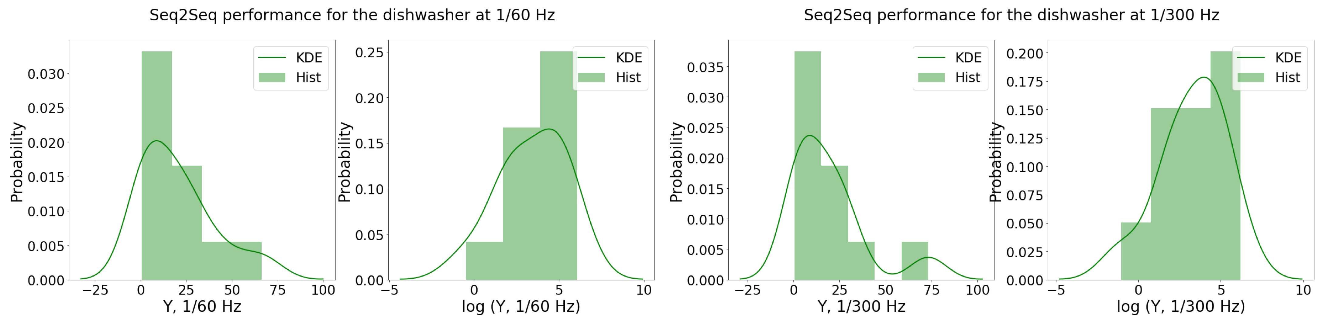
5.1.2. Dishwasher
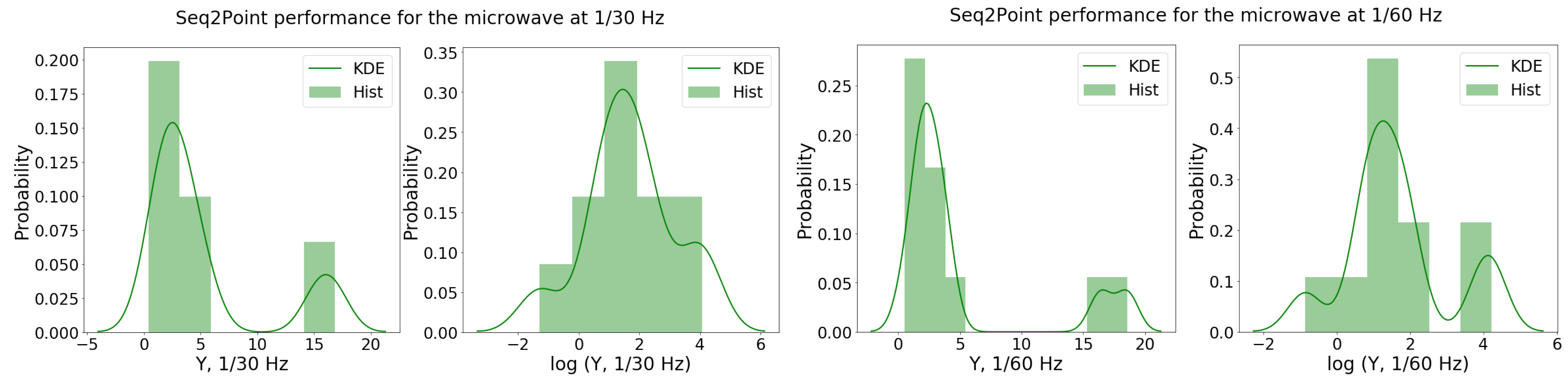
5.1.3. Microwave
5.2. Discussion
6. Conclusions
6.1. Research Implications and Potential Applications
6.2. Limitations and Future Work
Author Contributions
Funding
Institutional Review Board Statement
Informed Consent Statement
Data Availability Statement
Conflicts of Interest
Abbreviations
| AP | Number of appliances |
| BCT | Box–Cox transformation |
| BSS | Backward stepwise selection |
| D | Detached |
| DA | Dwelling age |
| DAE | Denoise autoencoder |
| DNN-NILM | Deep neural network NILM algorithms |
| DT | Dwelling type |
| DW | Dishwasher |
| KDE | Kernel density estimator |
| MAE | Mean absolute error |
| MT | Mid-terrace |
| MW | Microwave |
| NDE | Normalized disaggregation error |
| NILM | Non-intrusive load monitoring |
| OC | Number of occupants |
| RMSE | Root mean squared error |
| S | Dwelling size |
| S2P | Sequence-to-point |
| S2S | Sequence-to-sequence |
| SD | Semi-detached |
| TSKS | Two-sample Kolmogorov–Smirnov |
| UK | United Kingdom |
| WM | Washing machine |
References
- IEA. Electricity Information: Overview 2021. Available online: https://www.iea.org/reports/electricity-information-overview (accessed on 22 July 2022).
- Chakraborty, S.; Das, S.; Sidhu, T.; Siva, A. Smart meters for enhancing protection and monitoring functions in emerging distribution systems. Int. J. Electr. Power Energy Syst. 2021, 127, 106626. [Google Scholar] [CrossRef]
- Al-Waisi, Z.; Agyeman, M.O. On the challenges and opportunities of smart meters in smart homes and smart grids. In Proceedings of the 2nd International Symposium on Computer Science and Intelligent Control, Stockholm, Sweden, 21–23 September 2018; pp. 1–6. [Google Scholar]
- Batalla-Bejerano, J.; Trujillo-Baute, E.; Villa-Arrieta, M. Smart Meters and Consumer Behaviour: Insights from the Empirical Literature. Energy Policy 2020, 144, 111610. [Google Scholar] [CrossRef]
- Völker, B.; Reinhardt, A.; Faustine, A.; Pereira, L. Watt’s up at Home? Smart Meter Data Analytics from a Consumer-Centric Perspective. Energies 2021, 14, 719. [Google Scholar] [CrossRef]
- Gopinath, R.; Kumar, M.; Joshua, C.P.C.; Srinivas, K. Energy management using non-intrusive load monitoring techniques-State-of-the-art and future research directions. Sustain. Cities Soc. 2020, 62, 102411. [Google Scholar] [CrossRef]
- Majumdar, A. Trainingless Energy Disaggregation Without Plug-Level Sensing. IEEE Trans. Instrum. Meas. 2022, 71, 1–8. [Google Scholar] [CrossRef]
- Hart, G.W. Nonintrusive appliance load monitoring. Proc. IEEE 1992, 80, 1870–1891. [Google Scholar] [CrossRef]
- Iqbal, H.K.; Malik, F.H.; Muhammad, A.; Qureshi, M.A.; Abbasi, M.N.; Chishti, A.R. A critical review of state-of-the-art non-intrusive load monitoring datasets. Electr. Power Syst. Res. 2021, 192, 106921. [Google Scholar] [CrossRef]
- Batra, N.; Kukunuri, R.; Pandey, A.; Malakar, R.; Kumar, R.; Krystalakos, O.; Zhong, M.; Meira, P.; Parson, O. Towards reproducible state-of-the-art energy disaggregation. In Proceedings of the 6th ACM International Conference on Systems for Energy-Efficient Buildings, Cities, and Transportation, New York, NY, USA, 13–14 November 2019; pp. 193–202. [Google Scholar]
- Zhang, C.; Zhong, M.; Wang, Z.; Goddard, N.; Sutton, C. Sequence-to-point learning with neural networks for non-intrusive load monitoring. AAAI Conf. Artif. Intell. 2018, 32, 11873. [Google Scholar] [CrossRef]
- Nalmpantis, C.; Vrakas, D. Machine learning approaches for non-intrusive load monitoring: From qualitative to quantitative comparation. Artif. Intell. Rev. 2019, 52, 217–243. [Google Scholar] [CrossRef]
- Huchtkoetter, J.; Reinhardt, A. On the impact of temporal data resolution on the accuracy of non-intrusive load monitoring. In Proceedings of the 7th ACM International Conference on Systems for Energy-Efficient Buildings, Cities, and Transportation, Virtual. 18–20 November 2020; pp. 270–273. [Google Scholar]
- Huber, P.; Calatroni, A.; Rumsch, A.; Paice, A. Review on Deep Neural Networks Applied to Low-Frequency NILM. Energies 2021, 14, 2390. [Google Scholar] [CrossRef]
- Guo, Z.; Zhou, K.; Zhang, C.; Lu, X.; Chen, W.; Yang, S. Residential electricity consumption behavior: Influencing factors, related theories and intervention strategies. Renew. Sustain. Energy Rev. 2018, 81, 399–412. [Google Scholar] [CrossRef]
- Sena, B.; Zaki, S.A.; Rijal, H.B.; Alfredo Ardila-Rey, J.; Yusoff, N.M.; Yakub, F.; Ridwan, M.K.; Muhammad-Sukki, F. Determinant factors of electricity consumption for a Malaysian household based on a field survey. Sustainability 2021, 13, 818. [Google Scholar] [CrossRef]
- Karatasou, S.; Laskari, M.; Santamouris, M. Determinants of high electricity use and high energy consumption for space and water heating in European social housing: Socio-demographic and building characteristics. Energy Build. 2018, 170, 107–114. [Google Scholar] [CrossRef]
- Azlina, A.; Kamaludin, M.; Abdullah, E.S.Z.E.; Radam, A. Factors influencing household end-use electricity demand in Malaysia. Adv. Sci. Lett. 2016, 22, 4120–4123. [Google Scholar] [CrossRef]
- Navamuel, E.L.; Morollón, F.R.; Cuartas, B.M. Energy consumption and urban sprawl: Evidence for the Spanish case. J. Clean. Prod. 2018, 172, 3479–3486. [Google Scholar] [CrossRef]
- van den Brom, P.; Meijer, A.; Visscher, H. Performance gaps in energy consumption: Household groups and building characteristics. Build. Res. Inf. 2018, 46, 54–70. [Google Scholar] [CrossRef]
- Góis, J.; Pereira, L. A Novel Methodology for Identifying Appliance Usage Patterns in Buildings Based on Auto-Correlation and Probability Distribution Analysis. Energy Build. 2021, 256, 111618. [Google Scholar] [CrossRef]
- Hosseini, S.S.; Agbossou, K.; Kelouwani, S.; Cardenas, A. Non-intrusive load monitoring through home energy management systems: A comprehensive review. Renew. Sustain. Energy Rev. 2017, 79, 1266–1274. [Google Scholar] [CrossRef]
- Hosseini, S.; Kelouwani, S.; Agbossou, K.; Cardenas, A.; Henao, N. A semi-synthetic dataset development tool for household energy consumption analysis. In Proceedings of the 2017 IEEE International Conference on Industrial Technology (ICIT), Toronto, ON, Canada, 22–25 March 2017; pp. 564–569. [Google Scholar]
- Kong, X.; Zhu, S.; Huo, X.; Li, S.; Li, Y.; Zhang, S. A household energy efficiency index assessment method based on non-intrusive load monitoring data. Appl. Sci. 2020, 10, 3820. [Google Scholar] [CrossRef]
- Chen, D.; Irwin, D.; Shenoy, P. Smartsim: A device-accurate smart home simulator for energy analytics. In Proceedings of the 2016 IEEE International Conference on Smart Grid Communications (SmartGridComm), Sydney, Australia, 6–9 November 2016; pp. 686–692. [Google Scholar]
- Kaselimi, M.; Doulamis, N.; Voulodimos, A.; Protopapadakis, E.; Doulamis, A. Context aware energy disaggregation using adaptive bidirectional LSTM models. IEEE Trans. Smart Grid 2020, 11, 3054–3067. [Google Scholar] [CrossRef]
- Sambasivan, N.; Kapania, S.; Highfill, H.; Akrong, D.; Paritosh, P.; Aroyo, L.M. “Everyone wants to do the model work, not the data work”: Data Cascades in High-Stakes AI. In Proceedings of the 2021 CHI Conference on Human Factors in Computing Systems, Yokohama, Japan, 8–13 May 2021; pp. 1–15. [Google Scholar]
- Angelis, G.F.; Timplalexis, C.; Krinidis, S.; Ioannidis, D.; Tzovaras, D. NILM Applications: Literature review of learning approaches, recent developments and challenges. Energy Build. 2022, 261, 111951. [Google Scholar] [CrossRef]
- Jiang, Y.; Liu, M. Design of A Reliable Algorithmic with Deep Learning and Transfer Learning for Load Combination Recognition. In Proceedings of the 2021 8th International Conference on Dependable Systems and Their Applications (DSA), Yinchuan, China, 5–6 August 2021; pp. 541–550. [Google Scholar]
- Batra, N.; Singh, A.; Whitehouse, K. Gemello: Creating a detailed energy breakdown from just the monthly electricity bill. In Proceedings of the 22nd ACM SIGKDD International Conference on Knowledge Discovery and Data Mining, San Francisco, CA, USA, 13–17 August 2016; pp. 431–440. [Google Scholar]
- Batra, N.; Wang, H.; Singh, A.; Whitehouse, K. Matrix factorisation for scalable energy breakdown. AAAI Conf. Artif. Intell. 2017, 31, 11179. [Google Scholar] [CrossRef]
- Batra, N.; Baijal, R.; Singh, A.; Whitehouse, K. How good is good enough? re-evaluating the bar for energy disaggregation. arXiv 2015, arXiv:1510.08713. [Google Scholar]
- Chatterjee, S.; Simonoff, J.S. Handbook of Regression Analysis with Applications in R, 2nd ed.; Wiley: Hoboken, NJ, USA, 2020. [Google Scholar]
- Montgomery, D.; Peck, E.; Vining, G. Introduction to Linear Regression Analysis, 6th ed.; Wiley: Hoboken, NJ, USA, 2021. [Google Scholar]
- Box, G.E.; Cox, D.R. An analysis of transformations. J. R. Stat. Soc. Ser. B (Methodological) 1964, 26, 211–243. [Google Scholar] [CrossRef]
- Shapiro, S.S.; Wilk, M.B. An analysis of variance test for normality (complete samples). Biometrika 1965, 52, 591–611. [Google Scholar] [CrossRef]
- Murray, D.; Stankovic, L.; Stankovic, V. An electrical load measurements dataset of United Kingdom households from a two-year longitudinal study. Sci. Data 2017, 4, 160122. [Google Scholar] [CrossRef]
- Pöchacker, M.; Egarter, D.; Elmenreich, W. Proficiency of power values for load disaggregation. IEEE Trans. Instrum. Meas. 2015, 65, 46–55. [Google Scholar] [CrossRef]
- Kelly, J.; Knottenbelt, W. Neural nilm: Deep neural networks applied to energy disaggregation. In Proceedings of the 2nd ACM International Conference on Embedded Systems for Energy-Efficient Built Environments, Seoul, Korea, 4–5 November 2015; pp. 55–64. [Google Scholar]
- Pereira, L.; Nunes, N. Performance evaluation in non-intrusive load monitoring: Datasets, metrics, and tools—A review. Wiley Interdiscip. Rev. Data Min. Knowl. Discov. 2018, 8, e1265. [Google Scholar] [CrossRef]
- Hodges, J.L. The significance probability of the Smirnov two-sample test. Ark. För Mat. 1958, 3, 469–486. [Google Scholar] [CrossRef]
- Egarter, D.; Pöchacker, M.; Elmenreich, W. Complexity of power draws for load disaggregation. arXiv 2015, arXiv:1501.02954. [Google Scholar]
- Krystalakos, O.; Nalmpantis, C.; Vrakas, D. Sliding window approach for online energy disaggregation using artificial neural networks. In Proceedings of the 10th Hellenic Conference on Artificial Intelligence, Patras, Greece, 9–12 July 2018; pp. 1–6. [Google Scholar]
- Beyertt, A.; Verwiebe, P.; Seim, S.; Milojkovic, F.; Müller-Kirchenbauer, J. Felduntersuchung zu Behavioral Energy Efficiency Potentialen von privaten Haushalten. 2020. Available online: https://zenodo.org/record/3855575#.Yx8-eXbMJPY (accessed on 6 June 2022).
- Zimmermann, J.P.; Evans, M.; Griggs, J.; King, N.; Harding, L.; Roberts, P.; Evans, C. Household Electricity Survey: A Study of Domestic Electrical Product Usage; Intertek Testing & Certification Ltd.: Leatherhead, UK, 2012; pp. 213–214. [Google Scholar]


| Houses | |||||||||||
|---|---|---|---|---|---|---|---|---|---|---|---|
| 2 | 3 | 5 | 6 | 9 | 10 | 11 | 13 | 15 | 18 | 20 | |
| OC | 4 | 2 | 4 | 2 | 2 | 4 | 1 | 4 | 1 | 2 | 2 |
| S | 3 | 3 | 4 | 4 | 3 | 3 | 3 | 4 | 3 | 3 | 3 |
| AP | 15 | 27 | 44 | 49 | 24 | 31 | 25 | 28 | 19 | 34 | 39 |
| DA | - | 1988 | 1878 | 2005 | 1919–1944 | 1919–1944 | 1945–1964 | post 2002 | 1965–1974 | 1965–1974 | 1965–1974 |
| DT | SD | D | MT | D | D | D | D | D | SD | D | D |
| MAE (1/60 Hz) | Indicators | |||||||||||||
|---|---|---|---|---|---|---|---|---|---|---|---|---|---|---|
| Houses | FBP | Median | Mean | |||||||||||
| 2 | 3 | 5 | 6 | 9 | 10 | 11 | 13 | 15 | 18 | 20 | ||||
| DAE | 0 | |||||||||||||
| S2P | 10 | |||||||||||||
| S2S | 1 | |||||||||||||
| MAE (1/300 Hz) | ||||||||||||||
| DAE | 0 | |||||||||||||
| S2P | 7 | |||||||||||||
| S2S | 4 | |||||||||||||
| MAE (1/60 Hz) | Indicators | |||||||||||||
|---|---|---|---|---|---|---|---|---|---|---|---|---|---|---|
| Houses | FBP | Median | Mean | |||||||||||
| 2 | 3 | 5 | 6 | 9 | 10 | 11 | 13 | 15 | 18 | 20 | ||||
| DAE | 2 | |||||||||||||
| S2P | 5 | |||||||||||||
| S2S | 4 | |||||||||||||
| MAE (1/300 Hz) | ||||||||||||||
| DAE | 1 | |||||||||||||
| S2P | 3 | |||||||||||||
| S2S | 7 | |||||||||||||
| MAE (1/30 Hz) | Indicators | |||||||||||||
|---|---|---|---|---|---|---|---|---|---|---|---|---|---|---|
| Houses | FBP | Median | Mean | |||||||||||
| 2 | 3 | 5 | 6 | 9 | 10 | 11 | 13 | 15 | 18 | 20 | ||||
| DAE | 0 | |||||||||||||
| S2P | 5 | |||||||||||||
| S2S | 5 | |||||||||||||
| MAE (1/60 Hz) | ||||||||||||||
| DAE | 1 | |||||||||||||
| S2P | 6 | |||||||||||||
| S2S | 4 | |||||||||||||
| Appliance | Significant Effects | Irrelevant Effects |
|---|---|---|
| Washing Machine | OC(+) | S,DT, APP |
| Dishwasher | OC(+), (−) | S, APP |
| Microwave | S(+) | OC, APP, DT |
Publisher’s Note: MDPI stays neutral with regard to jurisdictional claims in published maps and institutional affiliations. |
© 2022 by the authors. Licensee MDPI, Basel, Switzerland. This article is an open access article distributed under the terms and conditions of the Creative Commons Attribution (CC BY) license (https://creativecommons.org/licenses/by/4.0/).
Share and Cite
Góis, J.; Pereira, L.; Nunes, N. A Data-Centric Analysis of the Impact of Non-Electric Data on the Performance of Load Disaggregation Algorithms. Sensors 2022, 22, 6914. https://doi.org/10.3390/s22186914
Góis J, Pereira L, Nunes N. A Data-Centric Analysis of the Impact of Non-Electric Data on the Performance of Load Disaggregation Algorithms. Sensors. 2022; 22(18):6914. https://doi.org/10.3390/s22186914
Chicago/Turabian StyleGóis, João, Lucas Pereira, and Nuno Nunes. 2022. "A Data-Centric Analysis of the Impact of Non-Electric Data on the Performance of Load Disaggregation Algorithms" Sensors 22, no. 18: 6914. https://doi.org/10.3390/s22186914
APA StyleGóis, J., Pereira, L., & Nunes, N. (2022). A Data-Centric Analysis of the Impact of Non-Electric Data on the Performance of Load Disaggregation Algorithms. Sensors, 22(18), 6914. https://doi.org/10.3390/s22186914