


Evaluation of Three Feature Dimension Reduction Techniques for Machine Learning-Based Crop Yield Prediction Models


Abstract
1. Introduction
2. Feature Selection, Extraction, and Combination within ML-Based Crop Yield Prediction Models
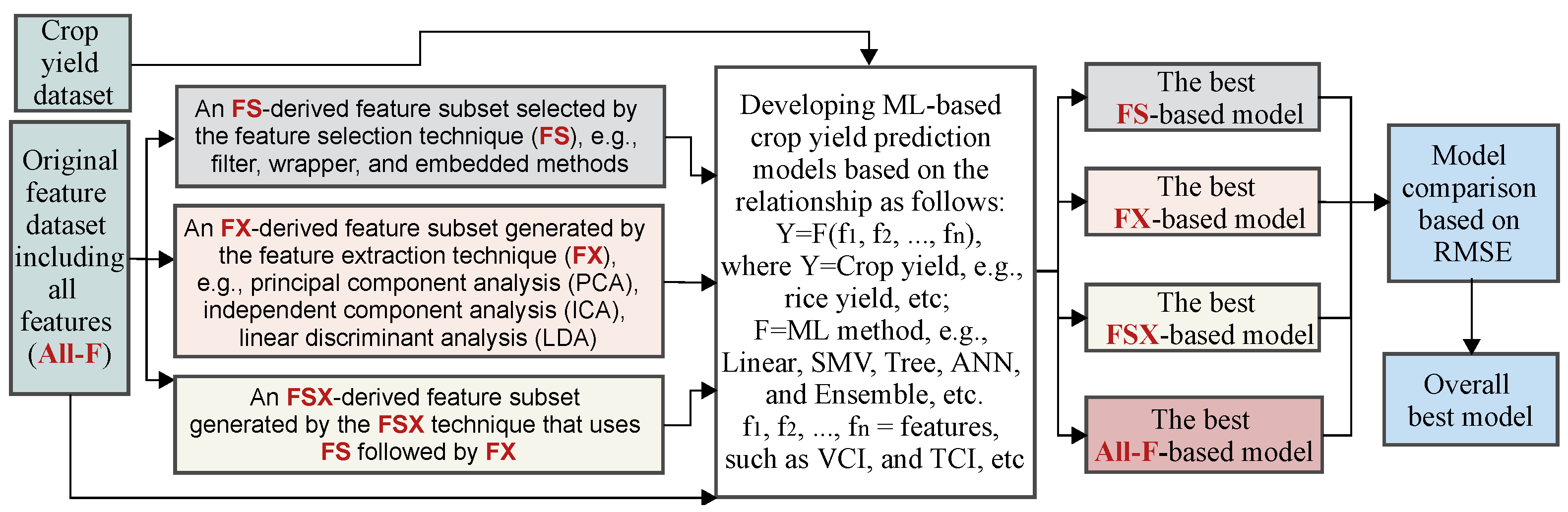
2.1. Problem Definition
2.2. Overview of Feature Selection (FS), Extraction (FX), and Combination (FSX)
2.2.1. Feature Selection
2.2.2. Feature Extraction
2.2.3. Feature Selection Combined with Feature Extraction (FSX)
3. Case Study of Vietnam’s Rice Yield Prediction
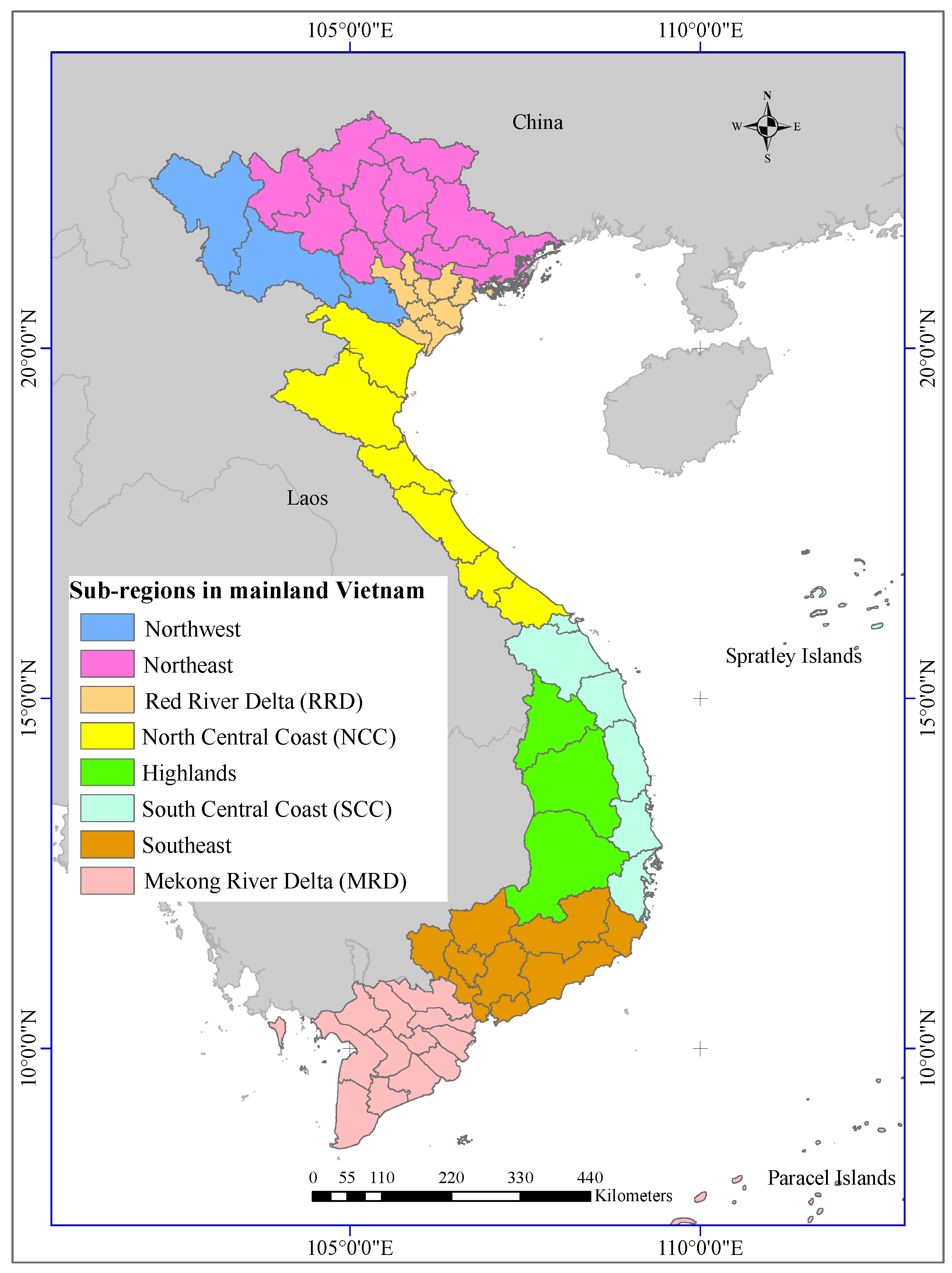
3.1. Study Area
3.2. Data
3.2.1. Annual Rice Yield in Vietnam
3.2.2. VCI/TCI Data
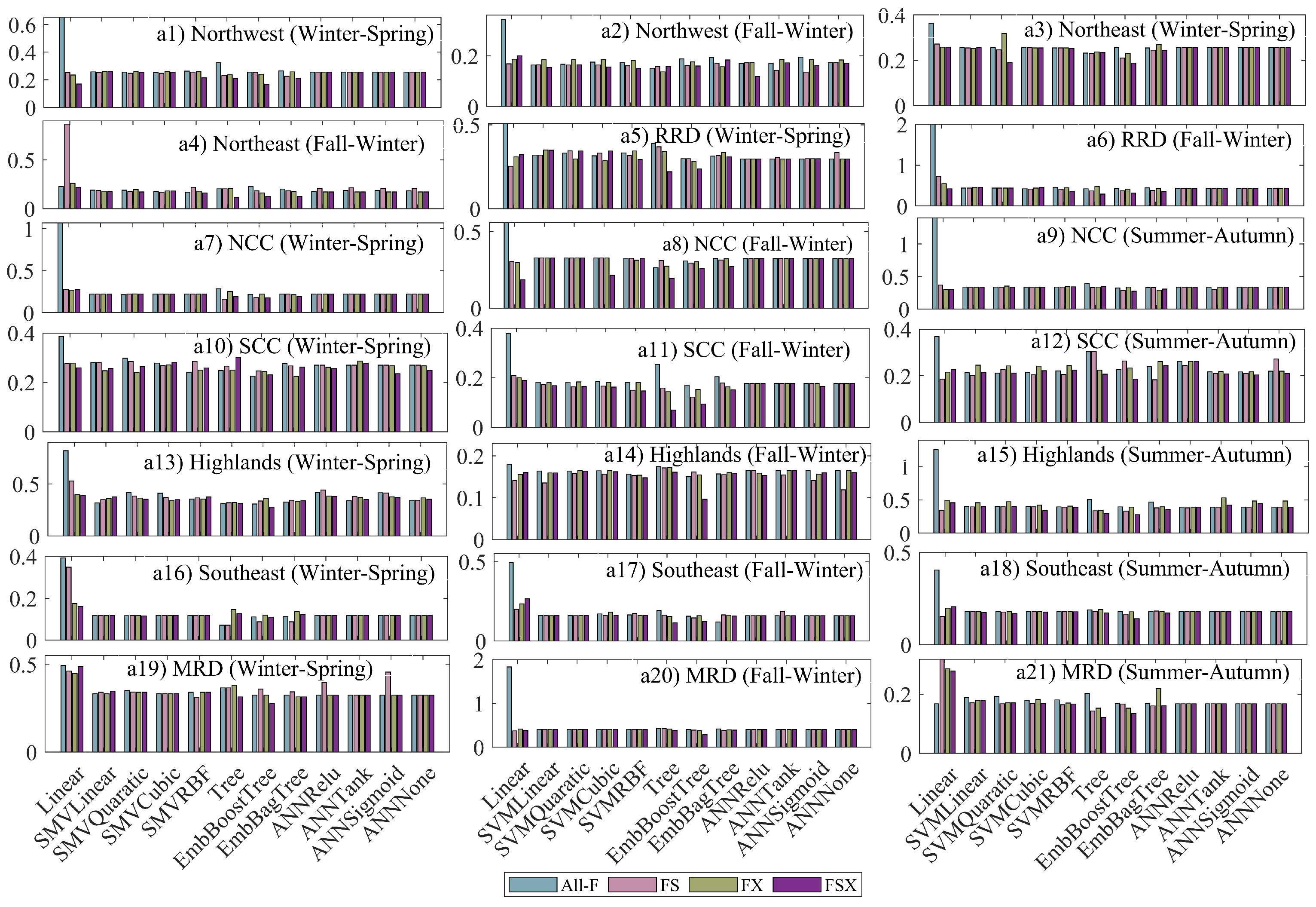
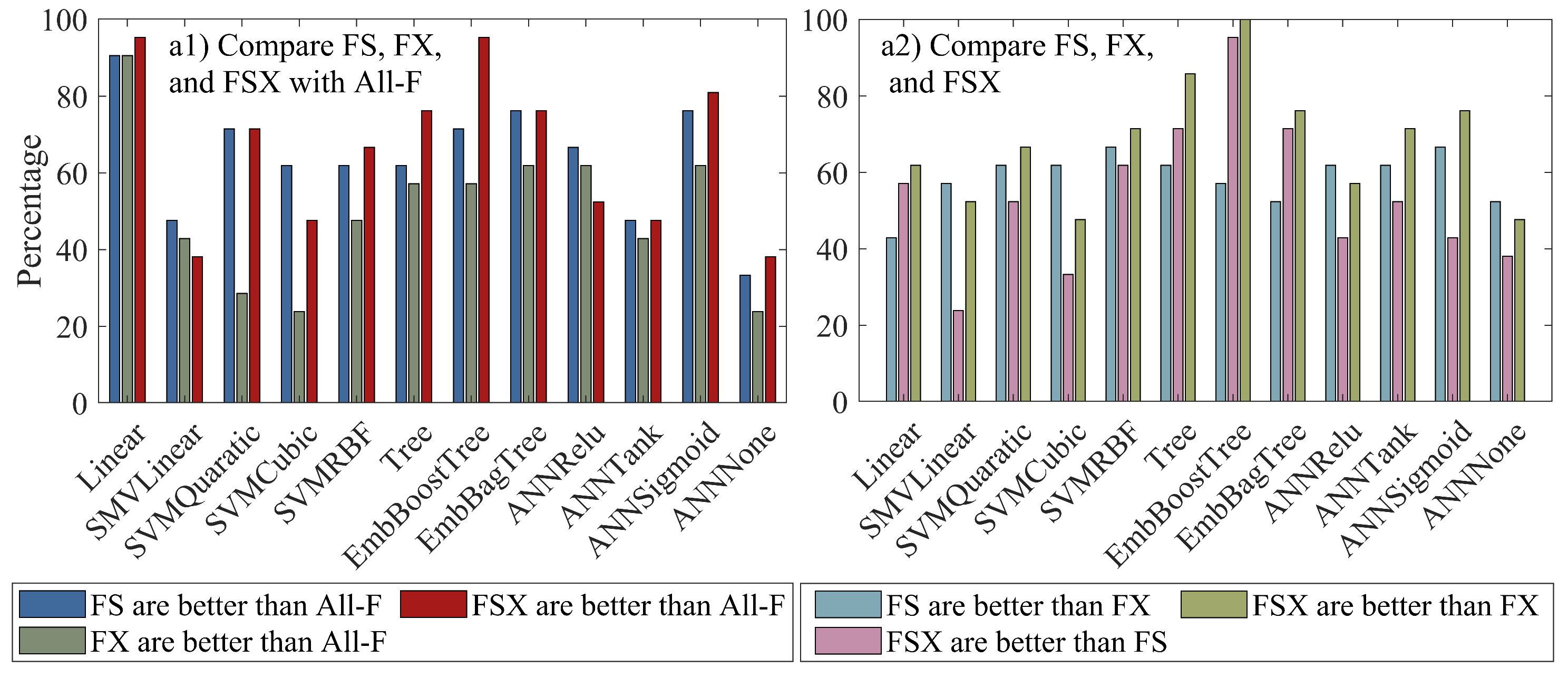
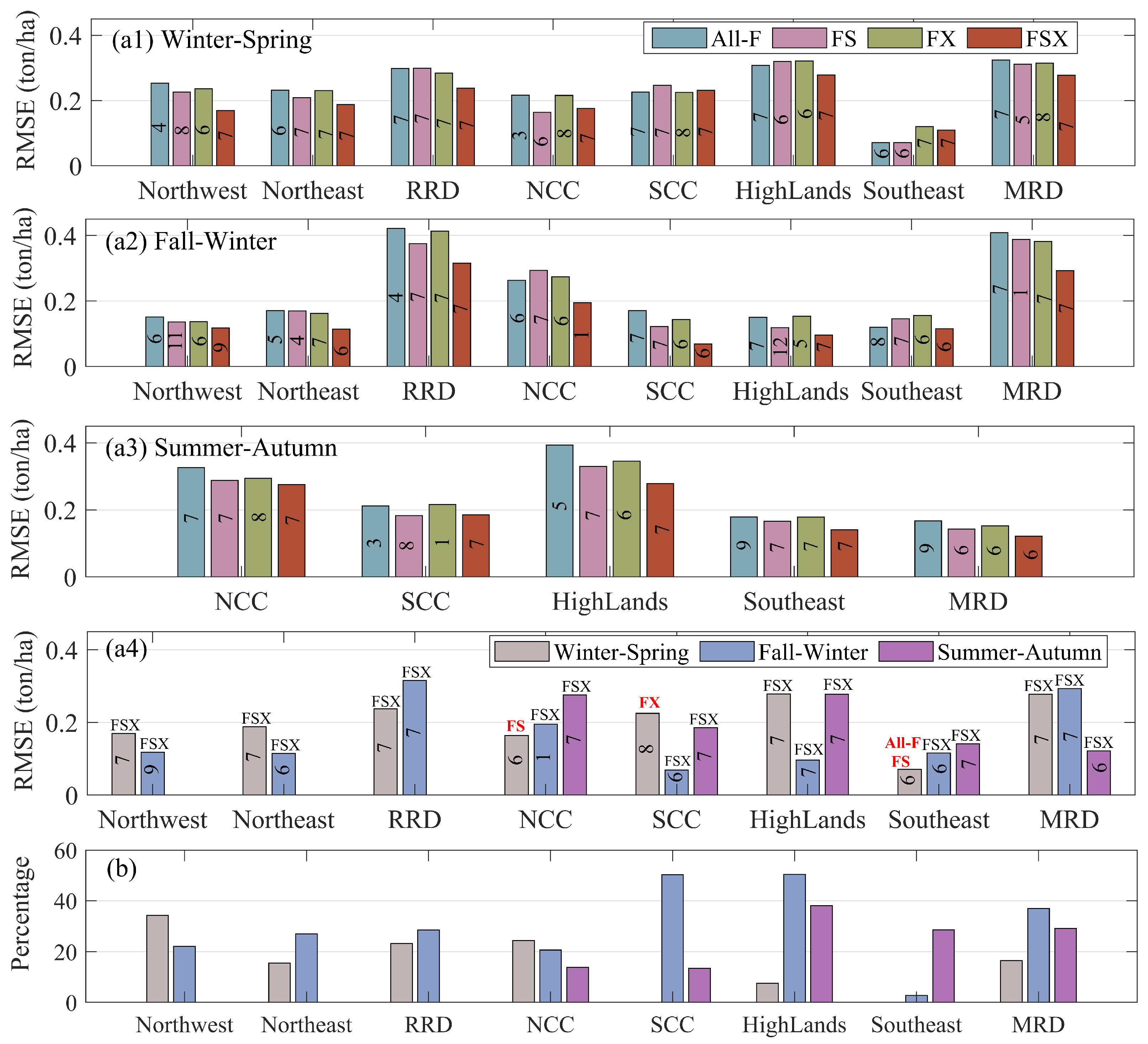
3.3. Results
4. Evaluation: Strengths and Limitations
5. Conclusions
Author Contributions
Funding
Institutional Review Board Statement
Informed Consent Statement
Data Availability Statement
Acknowledgments
Conflicts of Interest
Appendix A

| Crop; Regions | Features | Methods | Related Findings |
|---|---|---|---|
| Rice; Punjab State of India [9] | Features related to agriculture and weather | RRF; CBFS, RFE | Selected ten of the most significant features |
| Sugarcane; São Paulo State, Brazil [13] | NDVI: At the start, in the middle, 1–10 months after the harvest starts; amplitude; max; derivative; integral | Wrapper combining ANN | Selected seven essential features |
| Bio-oil; Unclear [15] | Biomass composition and pyrolysis conditions | GA, filter, wrapper | GA outperforms filter and wrapper methods. |
| Unclear crop; Tamil Nadu, India [8,14] | Canal length; the number of tanks, tube and open wells; planting area; amount of fertilizers, seed quantity; cumulative rainfall and radiation; max/average/min temperatures | FFS, BFE, CBFS, RFVarImp, VIF | Methods were quite the same accuracy (FFS and BFE are slightly better than others, but FFS takes less time) when combined with MLR and M5Prime but varied with ANN; The adjusted of 85% (84%) was achieved by using selected features (all features). |
| Unclear crop; Tamil Nadu, India [7] | Canal length; the number of tanks, tube and open wells; planting area; amount of fertilizers, seed quantity; cumulative rainfall and radiation; max/average/min temperatures | FFS, CBFS, VIF, RFVarImp | FFS gives good accuracy; RF achieves the highest quality for all feature subsets compared with ANN, SVM, and KNN. |
| Soybean; Southern France [17] | Features related to climate, soil, and management | Filter, wrapper, embedded | The subsets selected by wrapper combined with SVM and LR provided the best results. |
| Winter wheat; Germany [21,22] | Weekly weather data, soil conditions, and crop phenology variables | SHAP explanation | The accuracies of models using 50/75 percent of components did not decline significantly compared with the model using full features; some even slightly improved. |
| Corn, and Soybean; The United States [23] | Weather components, soil conditions, and management | The trained CNN-RNN model | The models’ accuracies did not decline remarkably compared to the model based on full features, but some even slightly improved. |
| Alfalfa, Wisconsin, the United States [19] | Vegetation indices | RFE | All models based on RF, SVM, and KNN were improved when using selected features. |
| Tee; Bangladesh [20] | Satellite-derived hydro-meteorological variables | Dragonfly and SVM | Combining RF with the dragonfly algorithm and SVR-based feature selection improves prediction performance. |
| Alfalfa; Kentucky and Georgia [16] | Weather, historical yield, sown date | CBFS, ReliefF, wrapper | CBFS was better than ReliefF and wrapper; ML combined with FS offered promise in forecasting performance. |
| Sugarcane; Teodoro Sampaio-São Paulo in Brazil [24] | Soil and weather | RReliefF | FS eliminated nearly 40% of the features but increased the mean absolute error (MAE) by 0.19 Mg/ha. |
| Coffee; Brazil [18] | Leaf area index (LAI), tree height, crown diameter, and the individual: RGB band values | Pearson, Spearman, F-test, RFE, Mutual Information | Most of the learners using the most important parameters (LAI and the crown diameter) and the most critical months improved prediction compared with employing total features. |
| Winter wheat, Corn; Kansas, USA [26,27] | VCI and TCI | PCA | The contribution of PCA was unclear because PCA-ML was not compared with ML-only. |
| Rice, Potato; Bangladesh [25,28] | VCI and TCI | PCA | The contribution of PCA was unclear because PCA-ML was not compared with ML-only. |
| Cotton; Unclear region [32] | Max/min temperature, relative humidity, wind speed, sunshine hours | PCA | A significant improvement in PCR-based prediction models compared with models using MLR. |
| Rice; Vietnam [33] | VCI and TCI | PCA | PCA coupled with EmbBoostTree was better than ML-only at an average of 18.5% and up to 45% of RMSE. |
References
- Filippi, P.; Jones, E.J.; Wimalathunge, N.S.; Somarathna, P.D.; Pozza, L.E.; Ugbaje, S.U.; Jephcott, T.G.; Paterson, S.E.; Whelan, B.M.; Bishop, T.F. An approach to forecast grain crop yield using multi-layered, multi-farm data sets and machine learning. Precis. Agric. 2019, 20, 1015–1029. [Google Scholar] [CrossRef]
- Van Klompenburg, T.; Kassahun, A.; Catal, C. Crop yield prediction using machine learning: A systematic literature review. Comput. Electron. Agric. 2020, 177, 105709. [Google Scholar] [CrossRef]
- Yang, Q.; Shi, L.; Han, J.; Zha, Y.; Zhu, P. Deep convolutional neural networks for rice grain yield estimation at the ripening stage using UAV-based remotely sensed images. Field Crops Res. 2019, 235, 142–153. [Google Scholar] [CrossRef]
- Zhong, L.; Hu, L.; Zhou, H. Deep learning based multi-temporal crop classification. Remote Sens. Environ. 2019, 221, 430–443. [Google Scholar] [CrossRef]
- Khalid, S.; Khalil, T.; Nasreen, S. A survey of feature selection and feature extraction techniques in machine learning. In Proceedings of the 2014 Science and Information Conference, London, UK, 27–29 August 2014; pp. 372–378. [Google Scholar] [CrossRef]
- Jia, W.; Sun, M.; Lian, J.; Hou, S. Feature dimensionality reduction: A review. Complex Intell. Syst. 2022, 8, 2663–2693. [Google Scholar] [CrossRef]
- Maya Gopal, P.S.; Bhargavi, R. Performance evaluation of best feature subsets for crop yield prediction using machine learning algorithms. Appl. Artif. Intell. 2019, 33, 621–642. [Google Scholar] [CrossRef]
- Maya Gopal, P.S.; Bhargavi, R. Selection of important features for optimizing crop yield prediction. Int. J. Agric. Environ. Inf. Syst. (IJAEIS) 2019, 10, 54–71. [Google Scholar] [CrossRef]
- Lingwal, S.; Bhatia, K.K.; Singh, M. A novel machine learning approach for rice yield estimation. J. Exp. Theor. Artif. Intell. 2022, 1–20. [Google Scholar] [CrossRef]
- Deng, H.; Runger, G. Gene selection with guided regularized random forest. Pattern Recognit. 2013, 46, 3483–3489. [Google Scholar] [CrossRef]
- Kowshalya, A.M.; Madhumathi, R.; Gopika, N. Correlation based feature selection algorithms for varying datasets of different dimensionality. Wirel. Pers. Commun. 2019, 108, 1977–1993. [Google Scholar] [CrossRef]
- Darst, B.F.; Malecki, K.C.; Engelman, C.D. Using recursive feature elimination in random forest to account for correlated variables in high dimensional data. BMC Genet. 2018, 19, 65. [Google Scholar] [CrossRef]
- Fernandes, J.L.; Ebecken, N.F.F.; Esquerdo, J.C.D.M. Sugarcane yield prediction in Brazil using NDVI time series and neural networks ensemble. Int. J. Remote Sens. 2017, 38, 4631–4644. [Google Scholar] [CrossRef]
- Gopal, P.M.; Bhargavi, R. Optimum feature subset for optimizing crop yield prediction using filter and wrapper approaches. Appl. Eng. Agric. 2019, 35, 9–14. [Google Scholar] [CrossRef]
- Ullah, Z.; Naqvi, S.R.; Farooq, W.; Yang, H.; Wang, S.; Vo, D.V.N. A comparative study of machine learning methods for bio-oil yield prediction—A genetic algorithm-based features selection. Bioresour. Technol. 2021, 335, 125292. [Google Scholar] [CrossRef] [PubMed]
- Whitmire, C.D.; Vance, J.M.; Rasheed, H.K.; Missaoui, A.; Rasheed, K.M.; Maier, F.W. Using machine learning and feature selection for alfalfa yield prediction. AI 2021, 2, 71–88. [Google Scholar] [CrossRef]
- Corrales, D.C.; Schoving, C.; Raynal, H.; Debaeke, P.; Journet, E.P.; Constantin, J. A surrogate model based on feature selection techniques and regression learners to improve soybean yield prediction in southern France. Comput. Electron. Agric. 2022, 192, 106578. [Google Scholar] [CrossRef]
- Barbosa, B.D.S.; Costa, L.; Ampatzidis, Y.; Vijayakumar, V.; dos Santos, L.M. UAV-based coffee yield prediction utilizing feature selection and deep learning. Smart Agric. Technol. 2021, 1, 100010. [Google Scholar] [CrossRef]
- Feng, L.; Zhang, Z.; Ma, Y.; Du, Q.; Williams, P.; Drewry, J.; Luck, B. Alfalfa yield prediction using UAV-based hyperspectral imagery and ensemble learning. Remote Sens. 2020, 12, 2028. [Google Scholar] [CrossRef]
- Jui, S.J.J.; Ahmed, A.M.; Bose, A.; Raj, N.; Sharma, E.; Soar, J.; Chowdhury, M.W.I. Spatiotemporal Hybrid Random Forest Model for Tea Yield Prediction Using Satellite-Derived Variables. Remote Sens. 2022, 14, 805. [Google Scholar] [CrossRef]
- Srivastava, A.K.; Safaei, N.; Khaki, S.; Lopez, G.; Zeng, W.; Ewert, F.; Gaiser, T.; Rahimi, J. Winter wheat yield prediction using convolutional neural networks from environmental and phenological data. Sci. Rep. 2022, 12, 3215. [Google Scholar] [CrossRef]
- Srivastava, A.K.; Safaei, N.; Khaki, S.; Lopez, G.; Zeng, W.; Ewert, F.; Gaiser, T.; Rahimi, J. Comparison of Machine Learning Methods for Predicting Winter Wheat Yield in Germany. arXiv 2021, arXiv:2105.01282. [Google Scholar]
- Khaki, S.; Wang, L.; Archontoulis, S.V. A CNN-RNN framework for crop yield prediction. Front. Plant Sci. 2020, 10, 1750. [Google Scholar] [CrossRef] [PubMed]
- Bocca, F.F.; Rodrigues, L.H.A. The effect of tuning, feature engineering, and feature selection in data mining applied to rainfed sugarcane yield modelling. Comput. Electron. Agric. 2016, 128, 67–76. [Google Scholar] [CrossRef]
- Rahman, A.; Khan, K.; Krakauer, N.; Roytman, L.; Kogan, F. Using AVHRR-based vegetation health indices for estimation of potato yield in Bangladesh. J. Civ. Environ. Eng. 2012, 2, 2. [Google Scholar] [CrossRef]
- Salazar, L.; Kogan, F.; Roytman, L. Using vegetation health indices and partial least squares method for estimation of corn yield. Int. J. Remote Sens. 2008, 29, 175–189. [Google Scholar] [CrossRef]
- Salazar, L.; Kogan, F.; Roytman, L. Use of remote sensing data for estimation of winter wheat yield in the United States. Int. J. Remote Sens. 2007, 28, 3795–3811. [Google Scholar] [CrossRef]
- Rahman, A.; Roytman, L.; Krakauer, N.Y.; Nizamuddin, M.; Goldberg, M. Use of vegetation health data for estimation of Aus rice yield in Bangladesh. Sensors 2009, 9, 2968–2975. [Google Scholar] [CrossRef]
- Jolliffe, I.T.; Cadima, J. Principal component analysis: A review and recent developments. Philos. Trans. R. Soc. A Math. Phys. Eng. Sci. 2016, 374, 20150202. [Google Scholar] [CrossRef]
- Awange, J.; Paláncz, B.; Völgyesi, L. Hybrid Imaging and Visualization; Springer International Publishing: Berlin/Heidelberg, Germany, 2020; p. 9. [Google Scholar]
- Preisendorfer, R.W.; Mobley, C.D. Principal component analysis in meteorology and oceanography. In Developments in Atmospheric Science; Elsevier: Amsterdam, The Netherlands, 1988; Volume 17. [Google Scholar]
- Suryanarayana, T.; Mistry, P. Principal Component Regression for Crop Yield Estimation; Springer: Singapore, 2016; p. 63. [Google Scholar]
- Pham, H.T.; Awange, J.; Kuhn, M.; Nguyen, B.V.; Bui, L.K. Enhancing Crop Yield Prediction Utilizing Machine Learning on Satellite-Based Vegetation Health Indices. Sensors 2022, 22, 719. [Google Scholar] [CrossRef]
- Liu, Z.; Japkowicz, N.; Wang, R.; Cai, Y.; Tang, D.; Cai, X. A statistical pattern based feature extraction method on system call traces for anomaly detection. Inf. Softw. Technol. 2020, 126, 106348. [Google Scholar] [CrossRef]
- Poornima, M.K.; Dheepa, G. An efficient feature selection and classification for the crop field identification: A hybridized wrapper based approach. Turk. J. Comput. Math. Educ. (TURCOMAT) 2022, 13, 241–254. [Google Scholar]
- Famili, A.; Shen, W.M.; Weber, R.; Simoudis, E. Data preprocessing and intelligent data analysis. Intell. Data Anal. 1997, 1, 3–23. [Google Scholar] [CrossRef]
- Liu, Y.; Zheng, Y.F. FS_SFS: A novel feature selection method for support vector machines. Pattern Recognit. 2006, 39, 1333–1345. [Google Scholar] [CrossRef]
- Maldonado, S.; Weber, R. A wrapper method for feature selection using support vector machines. Inf. Sci. 2009, 179, 2208–2217. [Google Scholar] [CrossRef]
- Zhao, Z.A.; Liu, H. Spectral Feature Selection for Data Mining; Taylor & Francis: Milton Park, UK, 2012. [Google Scholar] [CrossRef]
- Cateni, S.; Vannucci, M.; Vannocci, M.; Colla, V. Variable selection and feature extraction through artificial intelligence techniques. Multivar. Anal. Manag. Eng. Sci. 2012, 6, 103–118. [Google Scholar] [CrossRef]
- Wolpert, D.H.; Macready, W.G. No free lunch theorems for optimization. IEEE Trans. Evol. Comput. 1997, 1, 67–82. [Google Scholar] [CrossRef]
- Aurélien, G. Hands-On Machine Learning with Scikit-Learn & Tensorflow; O’Reilly Media, Inc.: Sebastopol, CA, USA, 2017. [Google Scholar]
- Opitz, D.; Maclin, R. Popular ensemble methods: An empirical study. J. Artif. Intell. Res. 1999, 11, 169–198. [Google Scholar] [CrossRef]
- Guyon, I.; Elisseeff, A. An introduction to variable and feature selection. J. Mach. Learn. Res. 2003, 3, 1157–1182. [Google Scholar] [CrossRef][Green Version]
- Suruliandi, A.; Mariammal, G.; Raja, S. Crop prediction based on soil and environmental characteristics using feature selection techniques. Math. Comput. Model. Dyn. Syst. 2021, 27, 117–140. [Google Scholar] [CrossRef]
- Zebari, R.; Abdulazeez, A.; Zeebaree, D.; Zebari, D.; Saeed, J. A comprehensive review of dimensionality reduction techniques for feature selection and feature extraction. J. Appl. Sci. Technol. Trends 2020, 1, 56–70. [Google Scholar] [CrossRef]
- Whitmire, C.D. Machine Learning and Feature Selection for Biomass Yield Prediction Using Weather and Planting Data. Ph.D. Thesis, University of Georgia, Athens, GA, USA, 2019. [Google Scholar]
- Veerabhadrappa, L.R. Multi-Level Dimensionality Reduction Methods Using Feature Selection and Feature Extraction. Int. J. Artif. Intell. Appl. (IJAIA) 2010, 1, 54–68. [Google Scholar] [CrossRef]
- Rangarajan, L. Bi-level dimensionality reduction methods using feature selection and feature extraction. Int. J. Comput. Appl. 2010, 4, 33–38. [Google Scholar] [CrossRef]
- Murphy, K.P. Machine Learning: A Probabilistic Perspective; MIT Press: Cambridge, MA, USA, 2012; p. 12. [Google Scholar]
- Cardoso, J.F. Dependence, correlation and gaussianity in independent component analysis. J. Mach. Learn. Res. 2003, 4, 1177–1203. [Google Scholar] [CrossRef]
- Hall, M.A.; Holmes, G. Benchmarking attribute selection techniques for discrete class data mining. IEEE Trans. Knowl. Data Eng. 2003, 15, 1437–1447. [Google Scholar] [CrossRef]
- Maclean, J.L.; Dawe, D.C.; Hettel, G.P. Rice Almanac: Source Book for the Most Important Economic Activity on Earth; International Rice Research Institute (IRRI): Los Baños, Philippines, 2002; p. 6. [Google Scholar]
- Thuy, N. Vietnam Remains World’s Second Largest Rice Exporter in 2021: USDA. Available online: https://hanoitimes.vn/vietnam-to-remain-worlds-second-largest-rice-exporter-in-2021-usda-317300.html (accessed on 29 August 2022).
- VGS Office. Agriculture, Forestry and Fishery. Available online: https://www.gso.gov.vn/Default20en.aspx?tabid=491 (accessed on 15 January 2021).
- Kogan, F.; Guo, W.; Yang, W.; Harlan, S. Space-based vegetation health for wheat yield modeling and prediction in Australia. J. Appl. Remote Sens. 2018, 12, 026002. [Google Scholar] [CrossRef]
- Kogan, F.N. Operational space technology for global vegetation assessment. Bull. Am. Meteorol. Soc. 2001, 82, 1949–1964. [Google Scholar] [CrossRef]
- Kogan, F.; Guo, W.; Yang, W. Drought and food security prediction from NOAA new generation of operational satellites. Geomat. Nat. Hazards Risk 2019, 10, 651–666. [Google Scholar] [CrossRef]
- Kogan, F.; Popova, Z.; Alexandrov, P. Early forecasting corn yield using field experiment dataset and Vegetation health indices in Pleven region, north Bulgaria. Ecologia i Industria (Ecol. Ind.) 2016, 9, 76–80. [Google Scholar] [CrossRef]
- Kogan, F.; Powell, A.; Fedorov, O. Use of Satellite and In-Situ Data to Improve Sustainability; Springer: Dordrecht, The Netherlands, 2011. [Google Scholar] [CrossRef]
- Kogan, F.N. Global drought watch from space. Bull. Am. Meteorol. Soc. 1997, 78, 621–636. [Google Scholar] [CrossRef]
- Kogan, F.; Salazar, L.; Roytman, L. Forecasting crop production using satellite-based vegetation health indices in Kansas, USA. Int. J. Remote Sens. 2012, 33, 2798–2814. [Google Scholar] [CrossRef]
- NOAA STAR. STAR-Global Vegetation Health Products. Available online: https://www.star.nesdis.noaa.gov/smcd/emb/vci/VH/vh_adminMean.php?type=Province_Weekly_MeanPlot (accessed on 15 December 2020).
- Sima, C.; Dougherty, E.R. What should be expected from feature selection in small-sample settings. Bioinformatics 2006, 22, 2430–2436. [Google Scholar] [CrossRef] [PubMed]
- Dash, M.; Liu, H. Feature selection for classification. Intell. Data Anal. 1997, 1, 131–156. [Google Scholar] [CrossRef]
- Macarof, P.; Bartic, C.; Groza, S.; Stătescu, F. Identification of drought extent using NVSWI and VHI in IAŞI county area, Romania. Aerul si Apa. Componente ale Mediului 2018, 2018, 53–60. [Google Scholar] [CrossRef]
- Jolliffe, I.T. Principal Component Analysis; Springer: New York, NY, USA, 2002; pp. 374–379. [Google Scholar]
- Draper, N.R.; Smith, H. Applied Regression Analysis; John Wiley and Sons: New York, NY, USA, 1981. [Google Scholar] [CrossRef]
- Shahhosseini, M.; Martinez-Feria, R.A.; Hu, G.; Archontoulis, S.V. Maize yield and nitrate loss prediction with machine learning algorithms. Environ. Res. Lett. 2019, 14, 124026. [Google Scholar] [CrossRef]
- Hassan, M.A.; Khalil, A.; Kaseb, S.; Kassem, M. Exploring the potential of tree-based ensemble methods in solar radiation modeling. Appl. Energy 2017, 203, 897–916. [Google Scholar] [CrossRef]
- Kang, Y.; Ozdogan, M.; Zhu, X.; Ye, Z.; Hain, C.; Anderson, M. Comparative assessment of environmental variables and machine learning algorithms for maize yield prediction in the US Midwest. Environ. Res. Lett. 2020, 15, 064005. [Google Scholar] [CrossRef]
- Obsie, E.Y.; Qu, H.; Drummond, F. Wild blueberry yield prediction using a combination of computer simulation and machine learning algorithms. Comput. Electron. Agric. 2020, 178, 105778. [Google Scholar] [CrossRef]
- Liu, Y.; Liu, Z.; Vu, H.L.; Lyu, C. A spatio-temporal ensemble method for large-scale traffic state prediction. Comput.-Aided Civ. Infrastruct. Eng. 2020, 35, 26–44. [Google Scholar] [CrossRef]
- Liu, Y.; Liu, Z.; Lyu, C.; Ye, J. Attention-based deep ensemble net for large-scale online taxi-hailing demand prediction. IEEE Trans. Intell. Transp. Syst. 2019, 21, 4798–4807. [Google Scholar] [CrossRef]


Publisher’s Note: MDPI stays neutral with regard to jurisdictional claims in published maps and institutional affiliations. |
© 2022 by the authors. Licensee MDPI, Basel, Switzerland. This article is an open access article distributed under the terms and conditions of the Creative Commons Attribution (CC BY) license (https://creativecommons.org/licenses/by/4.0/).
Share and Cite
Pham, H.T.; Awange, J.; Kuhn, M. Evaluation of Three Feature Dimension Reduction Techniques for Machine Learning-Based Crop Yield Prediction Models. Sensors 2022, 22, 6609. https://doi.org/10.3390/s22176609
Pham HT, Awange J, Kuhn M. Evaluation of Three Feature Dimension Reduction Techniques for Machine Learning-Based Crop Yield Prediction Models. Sensors. 2022; 22(17):6609. https://doi.org/10.3390/s22176609
Chicago/Turabian StylePham, Hoa Thi, Joseph Awange, and Michael Kuhn. 2022. "Evaluation of Three Feature Dimension Reduction Techniques for Machine Learning-Based Crop Yield Prediction Models" Sensors 22, no. 17: 6609. https://doi.org/10.3390/s22176609
APA StylePham, H. T., Awange, J., & Kuhn, M. (2022). Evaluation of Three Feature Dimension Reduction Techniques for Machine Learning-Based Crop Yield Prediction Models. Sensors, 22(17), 6609. https://doi.org/10.3390/s22176609