Article

Anisotropic SpiralNet for 3D Shape Completion and Denoising

Department of Computer Science and Engineering, Interdisciplinary Graduate Program in Medical Bigdata Convergence, Kangwon National University, Chuncheon 24341, Korea
*
Author to whom correspondence should be addressed.
These authors contributed equally to this work.
Sensors 2022, 22(17), 6457; https://doi.org/10.3390/s22176457
Submission received: 27 July 2022 / Revised: 22 August 2022 / Accepted: 22 August 2022 / Published: 27 August 2022
(This article belongs to the Collection Computational Imaging and Sensing)

Abstract

:
Three-dimensional mesh post-processing is an important task because low-precision hardware and a poor capture environment will inevitably lead to unordered point clouds with unwanted noise and holes that should be suitably corrected while preserving the original shapes and details. Although many 3D mesh data-processing approaches have been proposed over several decades, the resulting 3D mesh often has artifacts that must be removed and loses important original details that should otherwise be maintained. To address these issues, we propose a novel 3D mesh completion and denoising system with a deep learning framework that reconstructs a high-quality mesh structure from input mesh data with several holes and various types of noise. We build upon SpiralNet by using a variational deep autoencoder with anisotropic filters that apply different convolutional filters to each vertex of the 3D mesh. Experimental results show that the proposed method enhances the reconstruction quality and achieves better accuracy compared to previous neural network systems.

1. Introduction

Three-dimensional (3D) geometric data have consistently received much attention in the field of computer vision and graphics, and such data can be conveniently acquired by using various types of affordable 3D scanning [1] and depth camera devices. Most raw 3D shape data are represented as point clouds from low-cost hardware equipment. Three-dimensional mesh data structures that consist of numerous vertices, edges, and faces are also widely used in many industries and studies as well for the purposes of visualization, design, and manufacturing [2,3], as they are capable of efficiently storing 3D geometric shapes and reusing them. Converting 3D point cloud data into mesh data can be easily accomplished by making use of several commercial and public mesh libraries [4,5]. However, low-precision hardware and a poor capture environment will inevitably cause unordered point clouds with unwanted noise and holes that should be feasibly corrected while preserving the original shapes and details. Moreover, 3D mesh data converted from problematic point clouds are obviously not smooth and are unsuitable for use in isolation without additional post-processing steps such as 3D mesh completion and/or denoising.
The successful completion and refinement of a partial 3D mesh are known to be challenging and a crucial part of the modeling of high-quality industrial applications. Previous mesh filtering methods [6,7,8] mainly based on analytic approaches efficiently eliminate high-frequency noise in 3D mesh data and the geometric original details can simultaneously be retained. However, the parameters must be carefully chosen, and several instances of trial and error are mandatory before satisfactory results can be obtained. Moreover, new vertices that fully cover the partial meshes are seldom generated as they do not work very well when performing the shape completion task.
Recently, several studies have utilized convolutional neural networks (CNNs) to represent and process 3D mesh data. Convolutional mesh autoencoder (CoMA) [9] introduces spectral graph networks with Chebyshev filters to reduce the computational burden imposed by the high dimensional and large amount of training mesh data. However, transformation from the spatial to the spectral domain when training the networks results in a loss of the original shape of the mesh, thereby degrading the reconstruction accuracy. SpiralNet [10,11,12] outperforms CoMA owing to the well-designed spiral graph convolution operations. However, a spiral convolution filter with fixed coefficients is applied to the given mesh model and the representation power of the networks is therefore limited.
To overcome this issue, we propose a novel anisotropic graph convolution-based deep learning framework that performs 3D shape completion and refinement in a fully automatic manner (Figure 1). We utilize a graph convolutional autoencoder capable of extracting meaningful features from the mesh training data at each convolutional layer by locally observing the features to produce high-quality results. Specifically, we build the network upon SpiralNet to generate fine-grained and smooth meshes from the partial meshes with noise, and our anisotropic convolutions can apply a different filter to each vertex of the 3D mesh so as to improve the reconstruction power compared to previous CNN-based graph neural networks such as FeastNet, CoMA, and SpiralNets [9,10,11,12,13]. Inspired by the soft permutation of LSA-Conv [14], we model the spiral convolution weight matrix as a linear combination of the base matrices that are shared by all of the vertices of the 3D mesh. In contrast to conventional anisotropic filtering approaches that directly and independently apply different filters to each vertex, the method proposed here computes a small number of filter bases and corresponding coefficients for each vertex. Given that a typical 3D-scanned mesh has various types of noise and discontinuities, our anisotropic filtering approach is well-suited for this type of scanned mesh data. Our mesh autoencoder consists of several convolutional layers and up-and-down sampling based on quadratic mesh simplification for the pooling operations, as shown in Figure 1 and Figure 2. We find that incomplete 3D meshes passing through previous mesh autoencoders are not fully reconstructed and that holes remain. To cope with this problem, we run the optimization in the prediction phase. More precisely, we begin with the initial latent variables from the neural example to the decoder input, after which we update the latent variables iteratively to fill the holes fully.
In order to validate our system, we qualitatively and quantitatively compare the proposed method with those in previous work. In the experiments conducted in this study, our system achieves better performance as the anisotropic filters significantly improve the representation power and maintain the original shape while removing noise and filling the holes. We believe that our system can be considered as an efficient tool for the post-processing of scanned and captured 3D mesh data with randomly distributed noise and holes.

2. Related Work

Mesh restoration and modeling are important tasks in the computer vision and graphics field. Mesh-smoothing algorithms with the Poisson equation introduced earlier [15,16] are suitable for recovering small hole regions, but they do not work very well when handling larger ones. The linear 3D morphable model [17] learns 3D facial models obtained through scanning and expresses the texture and shape of the face in its partial space by using principal component analysis (PCA). SCAPE [18], one of the most well-known body models, utilizes PCA and runs a quadratic optimization process to represent natural human body postures. FLAME [19] can adjust facial expressions by using linear blend shapes with jaw and neck articulation. Most of these morphable models linearly represent the human body model, whereas the proposed approach effectively models the non-linearity of the human body structure by using well-designed deep learning frameworks.
Recently, deep-learning-based approaches have been attracting attention in the area of mesh data processing. For example, CNNs [20] have achieved great success in the image processing and computer vision fields [21]. CNNs are capable of learning the translation-invariant localized features of the training data. Recently, there have also been studies of various 3D mesh data structures [22,23,24,25,26,27]. Graph convolutional networks (GCNs) [28,29,30], popular deep learning frameworks for training and representing mesh data, analyze the geometric relationships between each node and its neighbors in a graph structure. There are two different types of graph convolutional architectures: the spectral and spatial types. Spectral GCNs [31] undertake convolutions by using the eigen-decomposition of the pre-defined graph Laplacian matrix, eventually converting all information pertaining to the vertices in the spatial domain into the spectral domain. Defferrad et al. [32] effectively reduced the computational costs incurred when training graph-structured data by utilizing the Chebyshev polynomial, which recursively approximates the graph Fourier transform without direct eigen-decomposition. CoMA [9] employs spectral GCNs to establish a 3D mesh autoencoder that also contains upsampling and downsampling layers based on a mesh simplification approach [33]. FeaStNet [13] performs its convolution operation in the spatial domain, and Litany et al. [34] proposes a CNN-based variational autoencoder (VAE) [35] for the probabilistic modeling of the latent space. Similar to our approach, it iteratively optimizes the latent variables by minimizing the errors between selected valid input mesh vertices and the predicted vertices while fixing the autoencoder parameters.
Spiral neural networks [10,11,12] have recently shown better results for processing and representing 3D mesh data when compared to earlier GCN-based methods. SpiralNet [10] defines the spiral structure that connects the vertices along the spiral trajectory and accurately finds the correspondences between two 3D meshes that have the same geometry but a different topology based on long short-term memory (LSTM) networks with the spiral structure. Instead of randomly selecting spiral vertices [10], Bouritsas et al. [11] proposes new ordered spiral sequences with a fixed length, resulting in improved performance for 3D mesh reconstruction with a fixed topology. SpiralNet++ [12] performs the convolution operation of concatenating the mesh vertices following a spiral trajectory that is fed to the multi-layer perceptrons (MLP) without truncation or zero-padding to construct the spiral structure [11]. Similar to previous dilated convolutions [36,37], dilated spiral convolution [12] has also been introduced to improve the performance without increasing the size of the spiral convolution. However, identical convolution filter weights are applied to all vertices in those SpiralNet-based methods, whereas we apply different filters efficiently and independently to each vertex. Experimental results show that the proposed method outperforms existing SpiralNet structures in terms of handling the holes and noise in the scanned 3D mesh. Also, the prediction speed of our mesh autoencoder is faster than CoMA, LSAConv, and SDConv [38], and similar to SpiralNet++.

3. Method

We propose a novel deep learning system that efficiently and automatically fills the holes and gaps of a partial 3D mesh shape with noise. We employ a deep variational autoencoder [35] that consists of an encoder and a decoder to predict the fine-grained 3D mesh structure. A latent space that embeds the meaningful spectral and spatial features of the 3D mesh data to achieve accurate hole filling and noise reduction outcomes is well established after training the proposed deep variational autoencoder. The input of our deep autoencoder are the complete 3D mesh vertices X = [ x 0 , x 1 , , x N 1 ] R N × F and the output is Y = [ y 0 , y 1 , , y N 1 ] R N × F , where F is the feature dimension, F = 3 represents the XYZ values of each vertex, and N denotes the total number of mesh vertices. Figure 1 shows our deep variational autoencoder in detail. The input 3D mesh X is encoded as z = enc ( X ) in the latent space and the latent vector z R 64 is decoded into the output 3D mesh Y = dec ( z ) . In our system, there are six anisotropic spiral convolution layers; we add three up-and-down pooling layers and three linear layers to our neural network system, as shown in Figure 1. Specifically, SpiralNet++ [12] defines the k-ring and k-disk for each vertex v in the 3D mesh structure as follows:
0 -ring ( v ) = { v } , k -disk ( v ) = i = 0 , , k i -ring ( v ) , ( k + 1 ) -ring ( v ) = N ( k -ring ( v ) ) / k -disk ( v ) ,
where 0-ring represents the starting vertex to define spiral sequences and k-disk denotes a union of i-rings, where i = { 0 , , k } . Here, N ( V ) denotes the set of neighboring indices of the vertices in the set V and ( k + 1 ) -ring is a set of vertex indices from N ( V ) excluding those included in k-disk. The spiral sequences S ( v , l ) for a single vertex index v are the following ordered set:
S ( v , l ) ( 0 -ring , 1 -ring , 2 -ring , , k -ring ) ,
where S ( v , l ) includes only a part of k-ring to define the length of the spiral sequences as the user-defined length l. Figure 3 shows the vertices that form the spiral according to the length l.
The spiral convolution input can be defined as x i = j S ( v i , l ) x j , where the l vertex features included in the spiral sequences S ( v i , l ) of the starting vertex index v i are concatenated into a vector x i of the i-th vertex. The convolutional output y i is then computed with the vertex feature x i R F i n · l , convolution weight matrix W R F o u t × F i n · l , and bias vector b R F o u t according to Equation (2):
y i = W x i + b
.
LSA-Conv [14] constructs the vertex features X i = [ x i , 0 , x i , 1 , , x i , K 1 ] R K × F i n for each vertex and the corresponding local 1-ring neighbors, where K 1 is the number of neighbors for each convolutional layer. In addition, a trainable weight matrix P i R K × K is plugged into Equation (2) in a soft permutation form to sort the 1-ring neighbors for each vertex on the mesh. Therefore, the output y i is obtained by the equation below:
y i = W [ vec ( f ( P i X i ) ) ] + b ,
where vec converts the vertex feature matrix X into a column vector and f represents the non-linear activation function.
LSA-Conv [14] devised the idea of effectively sorting all vertices by approximating a set of weight matrices { P i } i = 0 N 1 R N × K × K as a linear combination of trainable basis matrices V R N × D , where the number of bases is D, which is significantly smaller than the number of vertices, N. Weight matrix parameterization enables the automatic sorting of each vertex so that graph convolution can perform well. We modify this approach to enhance the network representation power by using anisotropic spiral convolutional filters such that each vertex has a different and desired convolution filter. Instead of directly and independently applying different filters to each vertex, our subspace design computes a small number of filter bases and corresponding coefficients for each vertex. We linearly parameterize the convolution weights of SpiralNet++ [12] as follows:
W i = v i G b i = v i C y i = W i x i + b i ,
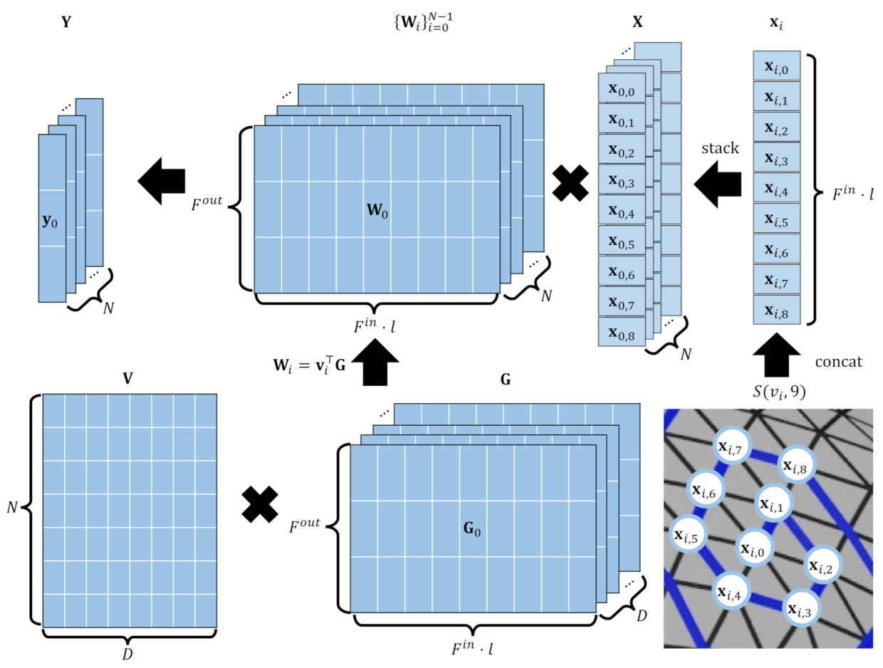
where { W i } i = 0 N 1 R N × F o u t × F i n · l includes spiral convolutional filters of length l for N vertices, as represented in G R D × F o u t × F i n · l and its corresponding coefficient matrix V = [ v 0 , v 1 , , v N 1 ] R N × D , which includes D-dimensional vectors. Here, B = [ b 0 , b 1 , , b N 1 ] R N × F o u t denotes the bias matrix, and each bias vector is also linearly parameterized with a vector of bases C R D × F o u t . The computational cost of our approach is similar to that in [12] while the reconstruction accuracy is greatly improved when compared to other neural network architectures, as ours allows locally anisotropic convolution filtering for all vertices on the 3D mesh. Figure 4 shows how our anisotropic spiral filter works.
The proposed deep variational autoencoder trains the encoder to build a variational distribution q ( z | X ) . The decoder is then trained to generate the resulting 3D mesh Y from the latent vector z . We train the neural network with the KL divergence and reconstruction L 2 losses. We use the normal distribution N ( 0 , I ) to make the variational distribution q ( z | X ) sample similarly as the prior distribution p ( z ) in the latent space. The loss function of our network to be minimized is φ ( X , Y ) λ KL ( q ( z | X ) p ( z ) ) , where φ is the Euclidean distance between X and Y with the L 2 norm and λ is a constant weight value for KL divergence. In our experiments, we set λ to 10 8 .
In the prediction phase, we iteratively optimize the decoder parameters only to reconstruct the incomplete 3D mesh faithfully. First, we generate the initial facial mesh to be optimized from the latent vector z that follows a normal distribution N ( 0 , I ) (see Figure 5b). Second, we pass the initial latent vector z into the decoder and the latent vector is optimized by iteratively solving X ^ Π ( dec ( z ) ) 2 2 , where X ^ is the incomplete input mesh (see Figure 5a) and Π is a selection matrix. Hence, the resulting output mesh Y * = dec ( z * ) is obtained from the optimal latent vector z * (see Figure 5c). We would like to refer the reader to [34] for the optimization of partial shape completion in detail.

4. Results

We quantitatively and qualitatively compared the proposed method with previous network systems such as CoMA, SpiralNet++, LSAConv, and SDConv, for the shape reconstruction and completion of the 3D mesh. We used two different datasets to train our neural networks. First, the MPI Dynamic FAUST dataset [39] includes full-body character motion. Our network was trained by using 37,557 frames out of a total of nearly 40,000 frames with a total of 10 actors and approximately 13 expressions, and was evaluated by using 3563 frames that were not used for training. The second dataset is CoMA, which includes various types of facial meshes of 18,845 frames with a total of 12 people and 12 expressions; our network was also evaluated for 1620 frames that were not included in the training dataset. All experiments were conducted by using PyTorch [40] on a system with an AMD Ryzen 9 5900X processor, 64 GB of memory, and an NVIDIA RTX 3080Ti GPU. The specific structures of the encoder and decoder are shown in Table 1. All networks were trained by using the Adam optimizer [41], and the learning rate of 0.001 and 100 epochs were utilized. For LSAConv and SDConv, 300 epochs were used.
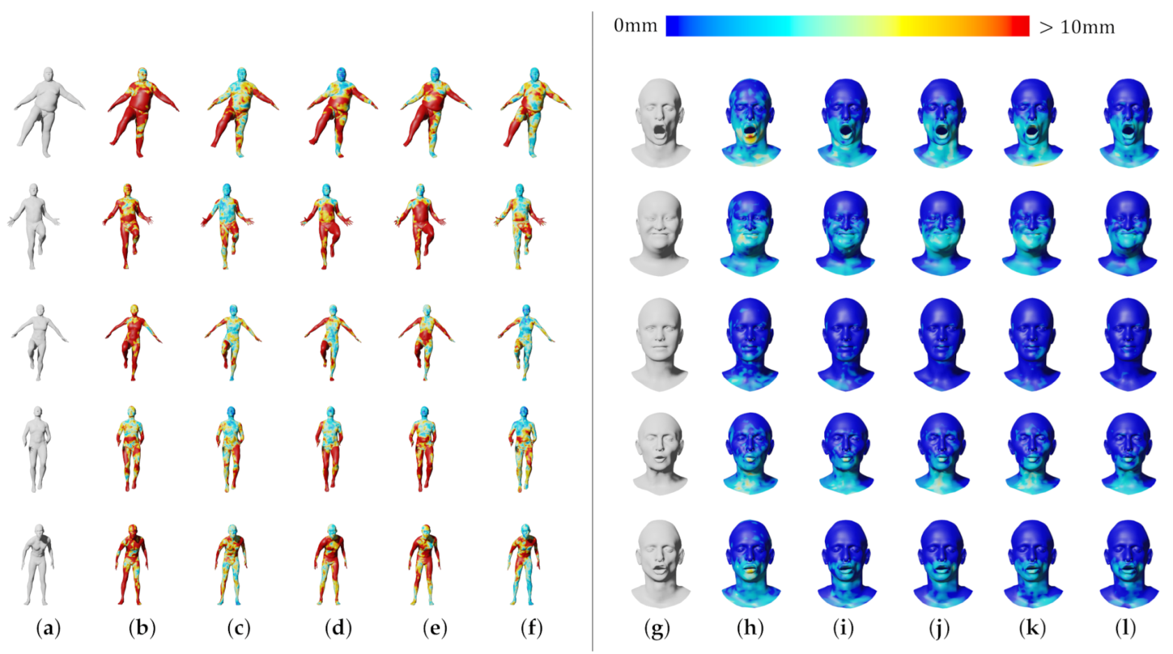
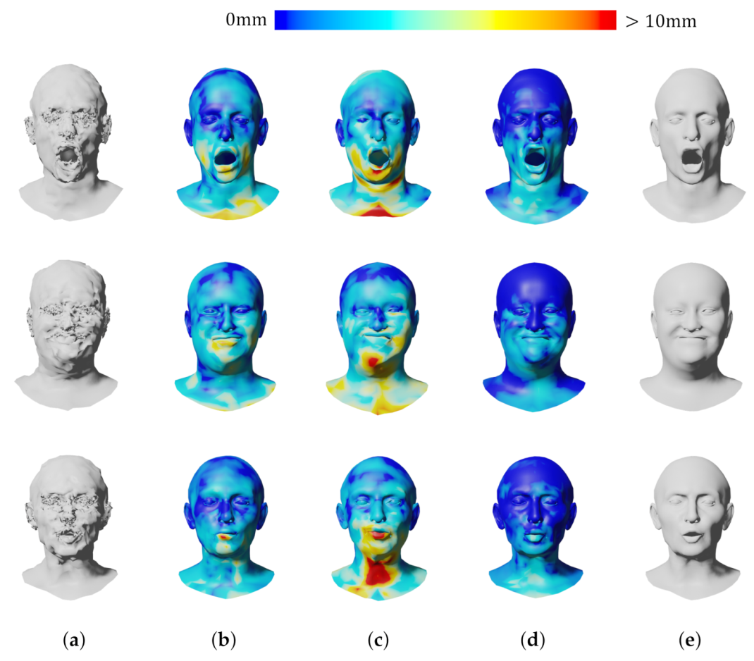
Table 2 and Figure 6 show the reconstruction errors compared to the other neural networks. The proposed network outperforms CoMA, SpiralNet++, and SDConv on 3D mesh reconstruction. Although our neural network has a bit more parameters than SpiralNet++, the prediction speed is similar to that of SpiralNet++ when performing the mesh reconstruction as our anisotropic convolution computation in Equation (4) is exactly same as the spiral one in Equation (2) other than computing with { W i , b i } . The precomputed { W i , b i } during the training step are reused in the prediction step, and we could not observe a meaningful prediction speed difference between ours and SpiralNet++. In addition, we synthetically and randomly added Gaussian noises on the input mesh data to test how well our system gets rid of the noises in the mesh data. In Figure 7, SpiralNet++ (Figure 7c) and CoMA (Figure 7b) successfully removed the given Gaussian noises, and CoMA showed better results than SpiralNet++. Our system achieved the smallest errors in every case that we have tested while preserving the original details of the mesh data (Figure 7d and Figure 8).
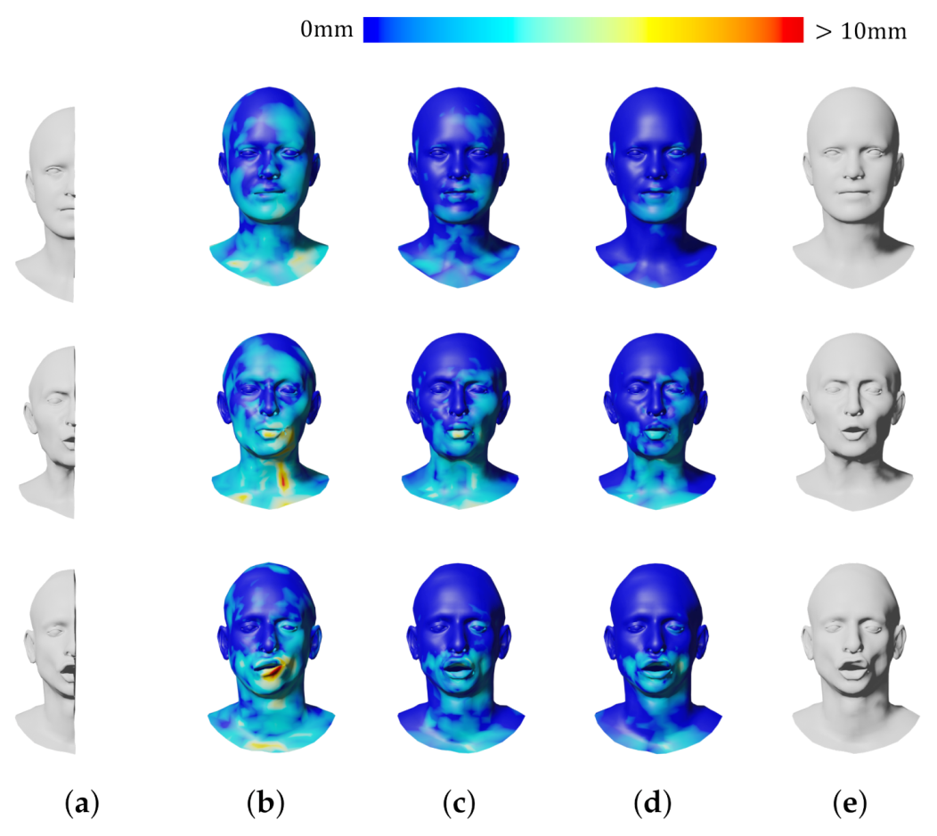
We also compared our approach with other networks for the 3D shape completion task and removed half of the vertices on the input mesh for the test. During the prediction step, the latent vector z was optimized 4000 times. We measured the average errors in each iteration (see Figure 8) and the average errors of the resulting mesh obtained at the last iteration (see Table 3). Figure 9 shows that CoMA (Figure 9b) generated a plausible overall shape of the mesh but did not produce expression details well. Meanwhile, SpiralNet++ (Figure 9c) showed better performance in terms of both overall shape completion and expressions, similar to the ground truth. However, some unnatural results were produced in the region of the lips that did not exist in the input mesh data. Our method (Figure 9d) successfully filled the holes and reconstructed the overall mesh shapes well while fewer error results occurred in missing regions of input mesh data. Table 3 presents comparisons of the 3D shape completion errors for each different mesh, where we find that the proposed method resulted in a smaller average error value compared to the other neural networks.

5. Conclusions

We have presented a novel anisotropic spiral neural network that faithfully reconstructs and completes a partial 3D mesh. We found that the proposed method could enhance the representation power owing to applying different convolutional filters to each vertex on 3D mesh. We show that our anisotropic filter can improve the reconstruction and shape completion accuracy for a facial and body mesh model. Our system can be useful for post-processing to obtain visually appealing mesh results without noticeable artifacts.
There will be several desirable future works. It would be interesting to extend our work to handle complex and arbitrary mesh structures mainly used in various engineering fields. We can apply the anisotropic spiral filters to other different types of data such as images and video sequences. Specifically, ours offers the possibility of successfully reconstructing the defective and noisy medical image data obtained from magnetic resonance imaging (MRI), computed tomography (CT), and ultrasonography [42]. Therefore, we believe that detecting abnormal tissues based on the post-processed medical image data from our model can be helpful to treat the patients. From the promising results in our work, we plan to establish a modified system that can handle highly dense mesh data as well as extremely problematic mesh data, in which it is difficult to differentiate original features from noise. To do so, we will incorporate attention mechanisms in our neural networks to achieve further improvement of the shape completion and denoise because they have the ability to selectively focus on relevant features during the training procedure.

Author Contributions

Conceptualization, S.U.K., J.R. and J.K.; software, S.U.K. and J.R.; validation, H.I. and J.K.; investigation, S.U.K. and J.R.; writing, S.U.K., J.R., H.I. and J.K.; supervision, J.K. All authors have read and agreed to the published version of the manuscript.

Funding

This work was supported by the National Research Foundation of Korea (NRF) grant funded by the Korea government (NRF-2022R1F1A1076095).

Institutional Review Board Statement

Not applicable.

Informed Consent Statement

Not applicable.

Data Availability Statement

Not applicable.

Conflicts of Interest

The authors declare no conflict of interest.

Abbreviations

The following abbreviations are used in this manuscript:
3DThree-dimensional
CNNConvolutional neural network
CoMAConvolutional mesh autoencoder
PCAPrincipal component analysis
GCNGraph convolutional network
LSTMLong short-term memory
MLPMulti-layer perceptron
MRIMagnetic Resonance Imaging
CTComputed Tomography

References

  1. Li, Y.; Guo, W.; Shen, J.; Wu, Z.; Zhang, Q. Motion-Induced Phase Error Compensation Using Three-Stream Neural Networks. Appl. Sci. 2022, 12, 8114. [Google Scholar] [CrossRef]
  2. Di Filippo, A.; Villecco, F.; Cappetti, N.; Barba, S. A Methodological Proposal for the Comparison of 3D Photogrammetric Models. In Proceedings of the Design Tools and Methods in Industrial Engineering II, Rome, Italy, 9–10 September 2021; Rizzi, C., Campana, F., Bici, M., Gherardini, F., Ingrassia, T., Cicconi, P., Eds.; Springer International Publishing: Cham, Switzerland, 2022; pp. 930–937. [Google Scholar]
  3. Jayathilakage, R.; Rajeev, P.; Sanjayan, J. Rheometry for Concrete 3D Printing: A Review and an Experimental Comparison. Buildings 2022, 12, 1190. [Google Scholar] [CrossRef]
  4. The CGAL Project. CGAL User and Reference Manual, 5.4th ed.; CGAL Editorial Board: Valbonne, France, 2022. [Google Scholar]
  5. Botsch, M.; Steinberg, S.; Bischoff, S.; Kobbelt, L. OpenMesh—A Generic and Efficient Polygon Mesh Data Structure. 2002. Available online: https://www.graphics.rwth-aachen.de/software/openmesh/ (accessed on 8 December 2020).
  6. Fleishman, S.; Drori, I.; Cohen-Or, D. Bilateral mesh denoising. In ACM SIGGRAPH 2003 Papers; Association for Computing Machinery: New York, NY, USA, 2003; pp. 950–953. [Google Scholar]
  7. Lee, K.W.; Wang, W.P. Feature-preserving mesh denoising via bilateral normal filtering. In Proceedings of the Ninth International Conference on Computer Aided Design and Computer Graphics (CAD-CG’05), Hong Kong, China, 7–10 December 2005; p. 6. [Google Scholar]
  8. Hou, Q.; Bai, L.; Wang, Y. Mesh smoothing via adaptive bilateral filtering. In Proceedings of the International Conference on Computational Science, Atlanta, GA, USA, 22–25 May 2005; Springer: Berlin/Heidelberg, Germany, 2005; pp. 273–280. [Google Scholar]
  9. Ranjan, A.; Bolkart, T.; Sanyal, S.; Black, M.J. Generating 3D faces using Convolutional Mesh Autoencoders. In Proceedings of the European Conference on Computer Vision (ECCV), Munich, Germany, 8–14 September 2018; pp. 725–741. [Google Scholar]
  10. Lim, I.; Dielen, A.; Campen, M.; Kobbelt, L. A simple approach to intrinsic correspondence learning on unstructured 3D meshes. In Proceedings of the European Conference on Computer Vision (ECCV) Workshops, Munich, Germany, 8–14 September 2018. [Google Scholar]
  11. Bouritsas, G.; Bokhnyak, S.; Ploumpis, S.; Bronstein, M.; Zafeiriou, S. Neural 3D morphable models: Spiral convolutional networks for 3D shape representation learning and generation. In Proceedings of the IEEE/CVF International Conference on Computer Vision, Seoul, Korea, 27 October–2 November 2019; pp. 7213–7222. [Google Scholar]
  12. Gong, S.; Chen, L.; Bronstein, M.; Zafeiriou, S. Spiralnet++: A fast and highly efficient mesh convolution operator. In Proceedings of the IEEE/CVF International Conference on Computer Vision Workshops, Seoul, Korea, 27 October–2 November 2019. [Google Scholar]
  13. Verma, N.; Boyer, E.; Verbeek, J. Feastnet: Feature-steered graph convolutions for 3D shape analysis. In Proceedings of the IEEE Conference on Computer Vision and Pattern Recognition, Salt Lake City, UT, USA, 18–22 June 2018; pp. 2598–2606. [Google Scholar]
  14. Gao, Z.; Yan, J.; Zhai, G.; Zhang, J.; Yang, Y.; Yang, X. Learning Local Neighboring Structure for Robust 3D Shape Representation. Proc. Aaai Conf. Artif. Intell. 2021, 35, 1397–1405. [Google Scholar]
  15. Kazhdan, M.; Hoppe, H. Screened poisson surface reconstruction. Acm Trans. Graph. 2013, 32, 1–13. [Google Scholar] [CrossRef]
  16. Zhao, W.; Gao, S.; Lin, H. A robust hole-filling algorithm for triangular mesh. Vis. Comput. 2007, 23, 987–997. [Google Scholar] [CrossRef]
  17. Blanz, V.; Vetter, T. A morphable model for the synthesis of 3D faces. In Proceedings of the 26th Annual Conference on Computer Graphics and Interactive Techniques, Los Angeles, CA, USA, 8–13 August 1999; pp. 187–194. [Google Scholar]
  18. Anguelov, D.; Srinivasan, P.; Koller, D.; Thrun, S.; Rodgers, J.; Davis, J. Scape: Shape completion and animation of people. In ACM SIGGRAPH 2005 Papers; Association for Computing Machinery: New York, NY, USA, 2005; pp. 408–416. [Google Scholar]
  19. Li, T.; Bolkart, T.; Black, M.J.; Li, H.; Romero, J. Learning a model of facial shape and expression from 4D scans. ACM Trans. Graph. 2017, 36, 194:1–194:17. [Google Scholar] [CrossRef]
  20. LeCun, Y.; Bottou, L.; Bengio, Y.; Haffner, P. Gradient-based learning applied to document recognition. Proc. IEEE 1998, 86, 2278–2324. [Google Scholar] [CrossRef]
  21. Azhar, I.; Sharif, M.; Raza, M.; Khan, M.A.; Yong, H.S. A Decision Support System for Face Sketch Synthesis Using Deep Learning and Artificial Intelligence. Sensors 2021, 21, 8178. [Google Scholar] [CrossRef] [PubMed]
  22. Achlioptas, P.; Diamanti, O.; Mitliagkas, I.; Guibas, L. Learning representations and generative models for 3D point clouds. In Proceedings of the International Conference on Machine Learning, PMLR, Stockholm, Sweden, 10–15 July 2018; pp. 40–49. [Google Scholar]
  23. Qi, C.R.; Su, H.; Mo, K.; Guibas, L.J. Pointnet: Deep learning on point sets for 3D classification and segmentation. In Proceedings of the IEEE Conference on Computer Vision and Pattern Recognition, Honolulu, HI, USA, 21–26 July 2017; pp. 652–660. [Google Scholar]
  24. Su, H.; Maji, S.; Kalogerakis, E.; Learned-Miller, E. Multi-view convolutional neural networks for 3D shape recognition. In Proceedings of the IEEE International conference on Computer Vision, Santiago, Chile, 11–18 December 2015; pp. 945–953. [Google Scholar]
  25. Wei, L.; Huang, Q.; Ceylan, D.; Vouga, E.; Li, H. Dense human body correspondences using convolutional networks. In Proceedings of the IEEE Conference on Computer Vision and Pattern Recognition, Las Vegas, NV, USA, 27–30 June 2016; pp. 1544–1553. [Google Scholar]
  26. Wu, Z.; Song, S.; Khosla, A.; Yu, F.; Zhang, L.; Tang, X.; Xiao, J. 3D shapenets: A deep representation for volumetric shapes. In Proceedings of the IEEE Conference on Computer Vision and Pattern Recognition, Boston, MA, USA, 7–12 June 2015; pp. 1912–1920. [Google Scholar]
  27. Wang, Y.; Sun, Y.; Liu, Z.; Sarma, S.E.; Bronstein, M.M.; Solomon, J.M. Dynamic graph CNN for learning on point clouds. Acm Trans. Graph. 2019, 38, 1–12. [Google Scholar] [CrossRef]
  28. Bronstein, M.M.; Bruna, J.; LeCun, Y.; Szlam, A.; Vandergheynst, P. Geometric deep learning: Going beyond Euclidean data. IEEE Signal Process. Mag. 2017, 34, 18–42. [Google Scholar] [CrossRef]
  29. Choi, H.; Moon, G.; Lee, K.M. Pose2mesh: Graph convolutional network for 3d human pose and mesh recovery from a 2d human pose. In Proceedings of the European Conference on Computer Vision, Glasgow, UK, 23–28 August 2020; Springer: Berlin/Heidelberg, Germany, 2020; pp. 769–787. [Google Scholar]
  30. Apicella, A.; Isgrò, F.; Pollastro, A.; Prevete, R. Dynamic filters in graph convolutional neural networks. arXiv 2021, arXiv:2105.10377. [Google Scholar]
  31. Bruna, J.; Zaremba, W.; Szlam, A.; LeCun, Y. Spectral networks and locally connected networks on graphs. arXiv 2013, arXiv:1312.6203. [Google Scholar]
  32. Defferrard, M.; Bresson, X.; Vandergheynst, P. Convolutional neural networks on graphs with fast localized spectral filtering. Adv. Neural Inf. Process. Syst. 2016, 29, 3844–3852. [Google Scholar]
  33. Garland, M.; Heckbert, P.S. Surface simplification using quadric error metrics. In Proceedings of the 24th Annual Conference on Computer Graphics and Interactive Techniques, Los Angeles, CA, USA, 3–8 August 1997; pp. 209–216. [Google Scholar]
  34. Litany, O.; Bronstein, A.; Bronstein, M.; Makadia, A. Deformable shape completion with graph convolutional autoencoders. In Proceedings of the IEEE Conference on Computer Vision and Pattern Recognition, Salt Lake City, UT, USA, 18–22 June 2018; pp. 1886–1895. [Google Scholar]
  35. Kingma, D.P.; Welling, M. Auto-encoding variational bayes. arXiv 2013, arXiv:1312.6114. [Google Scholar]
  36. Dutilleux, P. An implementation of the “algorithme à trous” to compute the wavelet transform. In Wavelets; Springer: Berlin/Heidelberg, Germany, 1990; pp. 298–304. [Google Scholar]
  37. Liang-Chieh, C.; Papandreou, G.; Kokkinos, I.; Murphy, K.; Yuille, A. Semantic Image Segmentation with Deep Convolutional Nets and Fully Connected CRFs. In Proceedings of the International Conference on Learning Representations, San Diego, CA, USA, 7–9 May 2015. [Google Scholar]
  38. Gao, Z.; Yan, J.; Zhai, G.; Yang, X. Learning Spectral Dictionary for Local Representation of Mesh. In Proceedings of the Thirtieth International Joint Conference on Artificial Intelligence, IJCAI-21, Montreal, QC, Canada, 19–27 August 2021; pp. 685–692. [Google Scholar] [CrossRef]
  39. Bogo, F.; Romero, J.; Pons-Moll, G.; Black, M.J. Dynamic FAUST: Registering Human Bodies in Motion. In Proceedings of the IEEE Conference on Computer Vision and Pattern Recognition (CVPR), Honolulu, HI, USA, 21–26 July 2017. [Google Scholar]
  40. Paszke, A.; Gross, S.; Massa, F.; Lerer, A.; Bradbury, J.; Chanan, G.; Killeen, T.; Lin, Z.; Gimelshein, N.; Antiga, L.; et al. PyTorch: An Imperative Style, High-Performance Deep Learning Library. In Advances in Neural Information Processing Systems 32; Curran Associates, Inc.: Red Hook, NY, USA, 2019; pp. 8024–8035. [Google Scholar]
  41. Kingma, D.P.; Ba, J. Adam: A method for stochastic optimization. arXiv 2014, arXiv:1412.6980. [Google Scholar]
  42. Mei, S.; Liu, M.; Kudreyko, A.; Cattani, P.; Baikov, D.; Villecco, F. Bendlet Transform Based Adaptive Denoising Method for Microsection Images. Entropy 2022, 24, 869. [Google Scholar] [CrossRef] [PubMed]
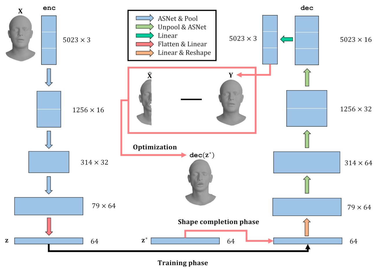
Figure 1. The architecture of the proposed model is based on anisotropic filters for 3D shape completion and denoising. In the prediction phase, we undertake partial shape completion, which iteratively optimizes the initial latent variable z by minimizing the errors between the valid parts of the input mesh and the corresponding predicted parts Y while holding the network parameters constant. The resulting output mesh Y * = dec ( z * ) is obtained by passing the optimal latent variable through a decoder.
Sensors 22 06457 g001
Figure 2. Mesh down- and upsampling results. The facial mesh (a) is downsampled for the pooling operation (b), then it is upsampled for the unpooling operation (c).
Sensors 22 06457 g002
Figure 3. Visualization of spiral sequences with different user parameter. (a) l = 9 ; (b) l = 12 ; (c) l = 15 ; (d) l = 18 ; (e) l = 21 .
Sensors 22 06457 g003
Figure 4. In the proposed anisotropic spiral convolution method, the spiral sequences S ( v i , l = 9 ) corresponding to the i-th vertex feature are concatenated from x i , 0 , x i , 1 , , x i , 8 ; this is denoted as x i . We linearly parameterize the convolutional filter weights { W i } i = 0 N 1 into the base matrices G R D × F o u t × F i n · l and their coefficients V R N × D to ensure that each vertex has a different and desired convolutional filter. In doing so, our method enhances the representation power compared to the conventional isotropic convolutional filters.
Sensors 22 06457 g004
Figure 5. The leftmost mesh shows the partial input mesh (a). The initial mesh is obtained by the decoder before performing network optimization (b), and the rightmost mesh shows the result obtained from the decoder after the iterative optimization step (c).
Sensors 22 06457 g005
Figure 6. Qualitative comparison of reconstruction errors. (af): DFAUST dataset, (gl): CoMA dataset. (a,g): Ground truth; (b,h): CoMA; (c,i): SpiralNet++; (d,j): LSAConv; (e,k): SDConv; (f,l): Ours.
Sensors 22 06457 g006
Figure 7. Qualitative comparison of shape denoising. (a) Input; (b) CoMA; (c) SpiralNet++; (d) Ours; (e) Ground truth.
Sensors 22 06457 g007
Figure 8. (a) This figure shows that our neural network system accomplishes faster convergence of the network optimization with fewer errors for the shape completion when compared with other neural network systems. (b) Our system achieves lower variance and errors than other neural network systems for the shape denoising task. All the errors are measured in millimeters.
Sensors 22 06457 g008
Figure 9. Qualitative comparison of shape completion. (a) Input; (b) CoMA; (c) SpiralNet++; (d) Ours; (e) Ground truth.
Sensors 22 06457 g009
Table 1. The architectures of our network and other neural networks tested in this paper (CoMA and SpiralNet++) are shown in detail. Note that ASNet represents our anisotropic convolutional filter shown in Figure 4 and that the input and output shapes of each layer are identical across all networks. * For variational autoencoder scheme, it requires two linear layers for mean ( μ R 64 ) and standard deviation ( σ R 64 ) .
CoMA / SpiralNet++ (Encoder)Ours (Encoder)
LayerInputOutputLayerInputOutput
CoMA/SpiralNet 5023 × 3 5023 × 16 ASNet 5023 × 3 5023 × 16
Pool 5023 × 16 1256 × 16 Pool 5023 × 16 1256 × 16
CoMA/SpiralNet 1256 × 16 1256 × 32 ASNet 1256 × 16 1256 × 32
Pool 1256 × 32 314 × 32 Pool 1256 × 32 314 × 32
CoMA/SpiralNet 314 × 32 314 × 64 ASNet 314 × 32 314 × 64
Pool 314 × 64 79 × 64 Pool 314 × 64 79 × 64
Flatten 79 × 64 1 × 5056 Flatten 79 × 64 1 × 5056
Linear 1 × 5056 1 × 64 *Linear 1 × 5056 1 × 64 *
CoMA / SpiralNet++ (Decoder)Ours (Decoder)
LayerInputOutputLayerInputOutput
Linear 1 × 64 1 × 5056 Linear 1 × 64 1 × 5056
Reshape 1 × 5056 79 × 64 Reshape 1 × 5056 79 × 64
Pool 79 × 64 314 × 64 Pool 79 × 64 314 × 64
CoMA/SpiralNet 314 × 64 314 × 64 ASNet 314 × 64 314 × 64
Pool 314 × 64 1256 × 64 Pool 314 × 64 1256 × 64
CoMA/SpiralNet 1256 × 64 1256 × 32 ASNet 1256 × 64 1256 × 32
Pool 1256 × 32 5023 × 32 Pool 1256 × 32 5023 × 32
CoMA/SpiralNet 5023 × 32 5023 × 16 ASNet 5023 × 32 5023 × 16
CoMA/SpiralNet 5023 × 16 5023 × 3 Linear 5023 × 16 5023 × 3
Table 2. Comparisons of the reconstruction errors, number of network parameters, and speed for CoMA, SpiralNet++, LSAConv, SDConv, and ours. All the reconstruction average errors are measured in millimeters.
NetworkDataset
DFAUSTCoMA
ErrorParamsFrame/secErrorParamsFrame/sec
CoMA12.4161390K 548.0 ± 5.4 0.66611031K 450.6 ± 8.6
SpiralNet++7.5101418K 1482.9 ± 24.9 0.42361059K 894.4 ± 8.7
LSAConv 110.4932540K 347.2 ± 3.4 0.42031723K 356.0 ± 3.0
SDConv 110.488564K 494.8 ± 2.4 0.4525443K 448.5 ± 5.1
Ours6.1512147K 1463.1 ± 24.3 0.35511750K 912.3 ± 8.4
1 Zhongpai Gao, https://github.com/Gaozhongpai/SDConvMesh. (accessed on 14 July 2022).
Table 3. Quantitative comparison of shape completion by using different actor models from the CoMA dataset. All the average errors are measured in millimeter (mm).
NetworkActor IDMean
013732720024013832743275012832763277327832790223
CoMA1.0731.1791.0571.1071.1610.8901.3061.0590.9990.9261.0400.8731.071
SpiralNet++0.4890.5680.5920.6750.6990.4600.7600.5940.5580.5160.6110.4730.603
Ours0.4470.5740.4950.5930.6250.3890.7590.5330.4740.4370.5300.4190.541
Publisher’s Note: MDPI stays neutral with regard to jurisdictional claims in published maps and institutional affiliations.