
Study on Accuracy Improvement of Slope Failure Region Detection Using Mask R-CNN with Augmentation Method


Abstract
:1. Introduction
2. Detection Model of Slope Failure Regions
2.1. Image Recognition Method
2.1.1. Slope Failure Monitoring
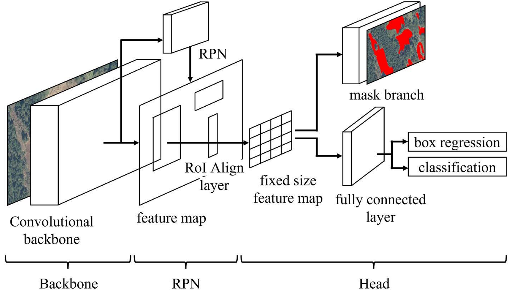
2.1.2. Mask R-CNN
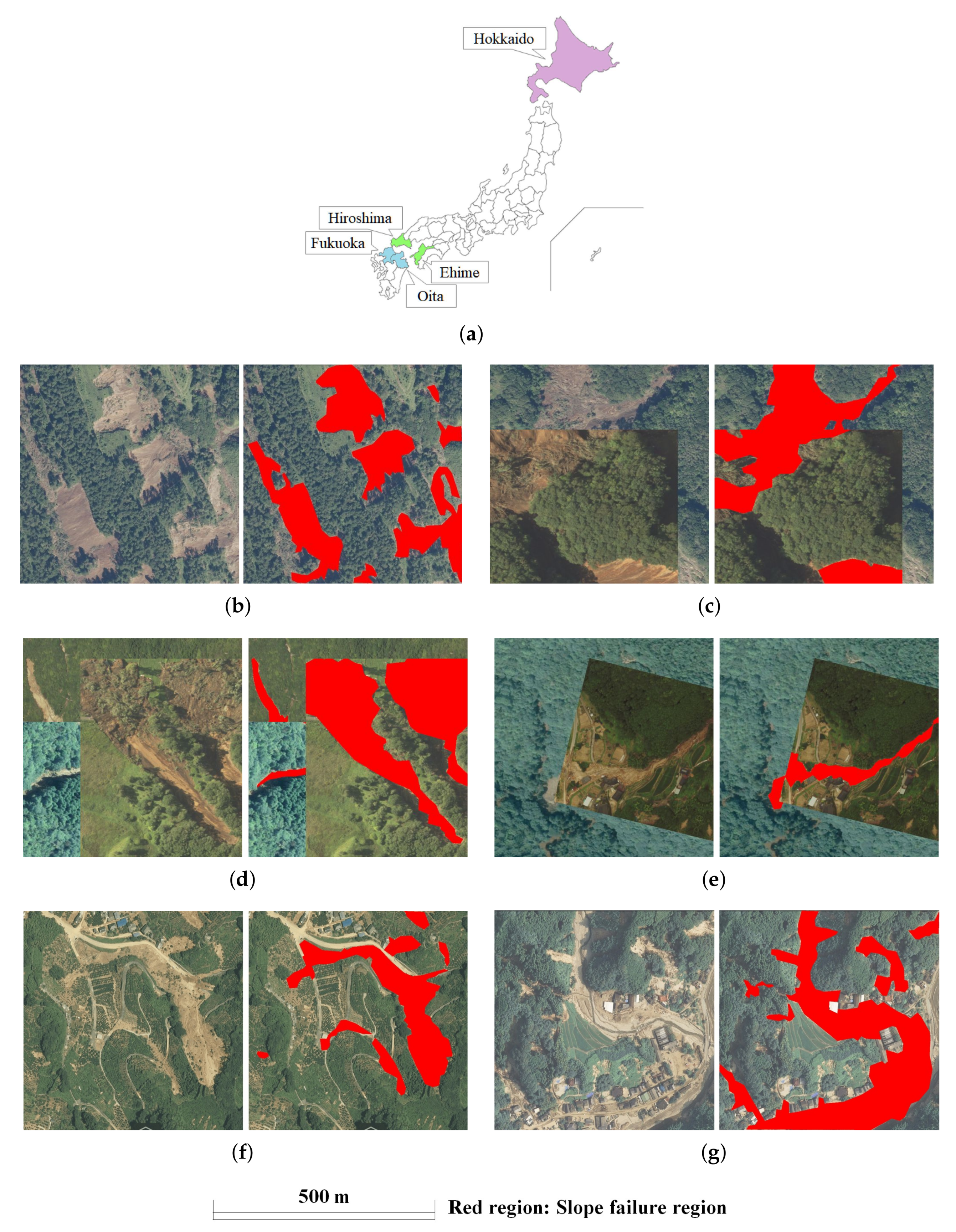
2.2. Datasets
2.3. Image Augmentation
2.4. Model Construction and Training
2.4.1. Construction of Semantic Segmentation Model
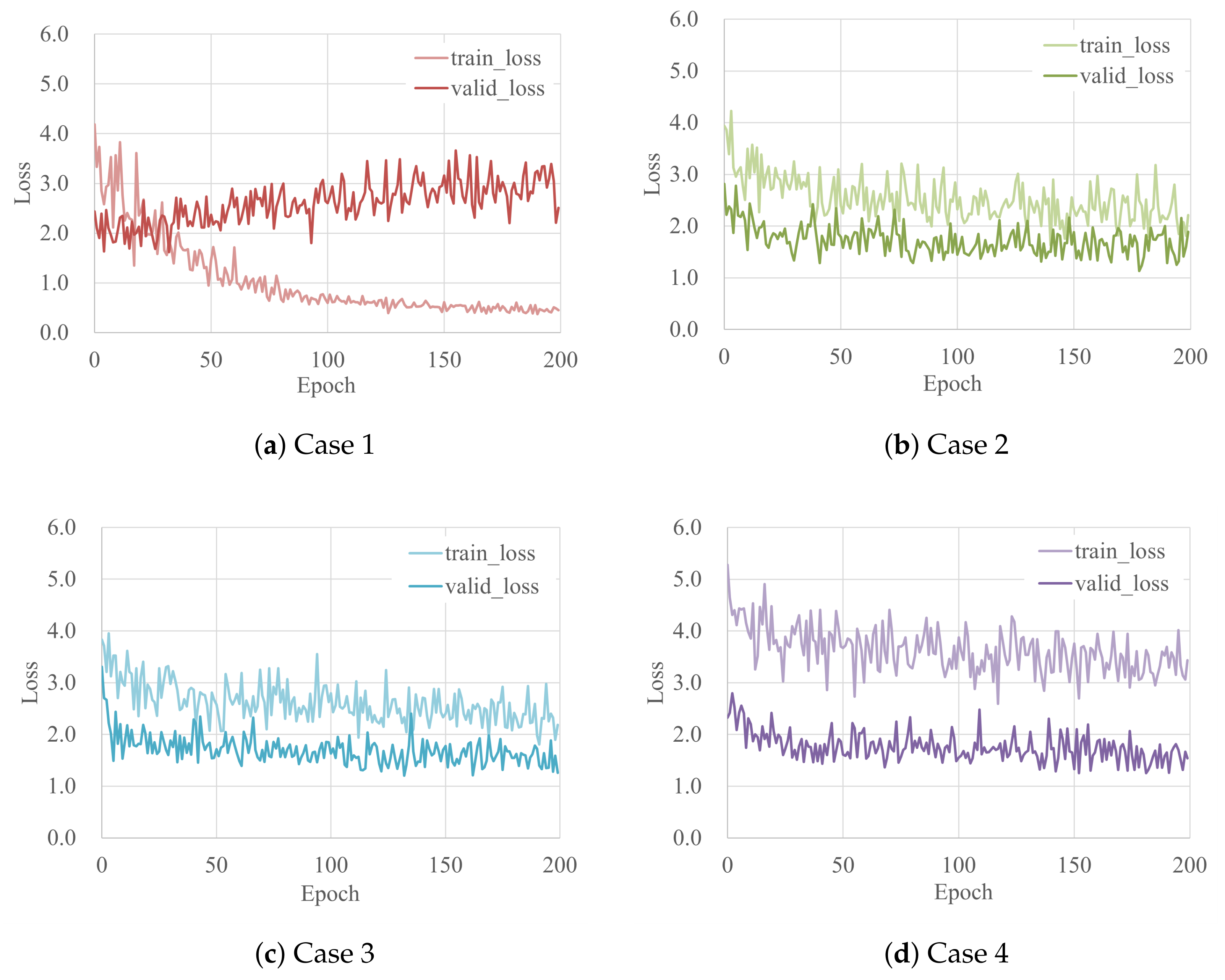
2.4.2. Cnn Training and Validation
3. Results of Detection
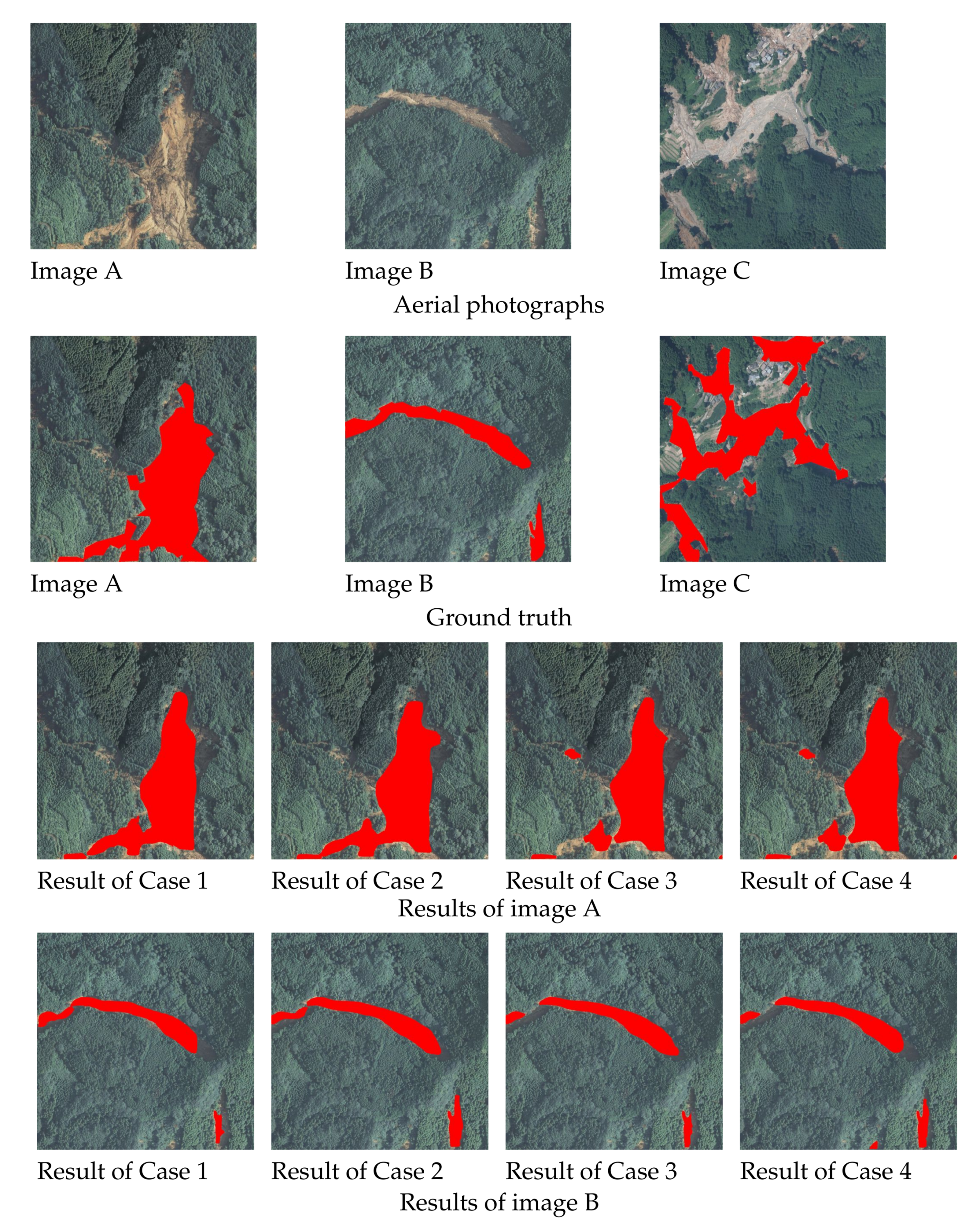
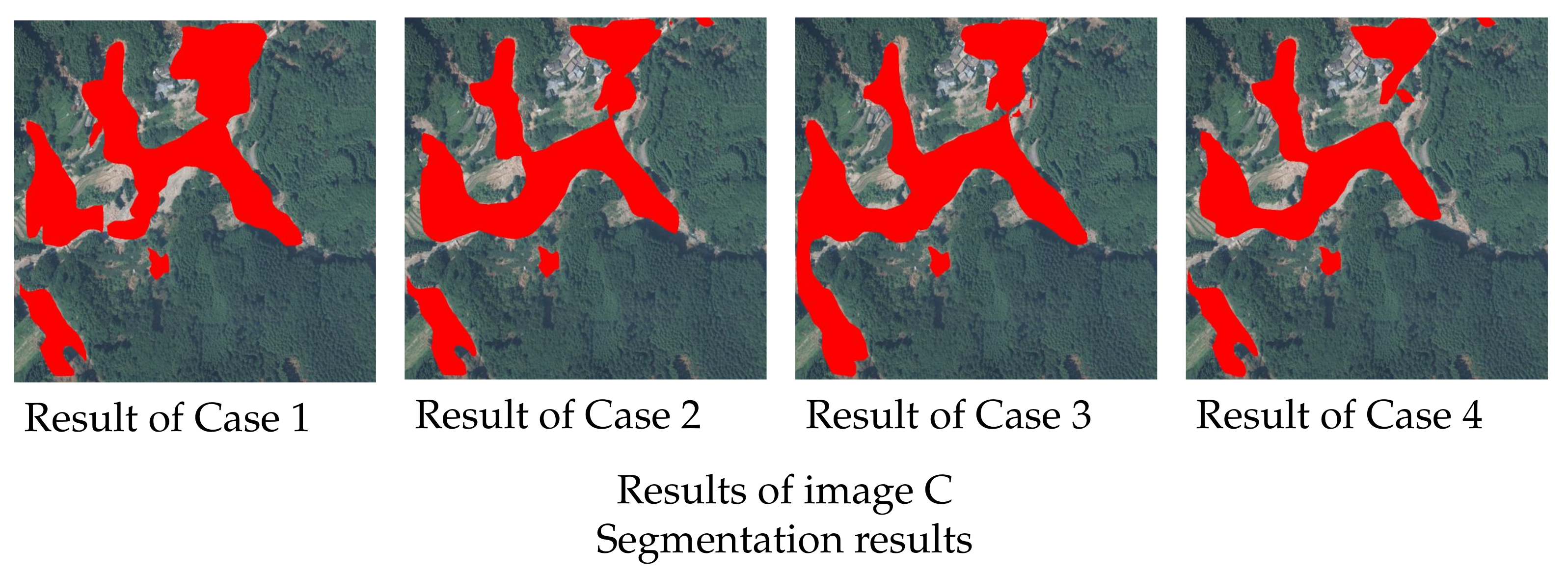
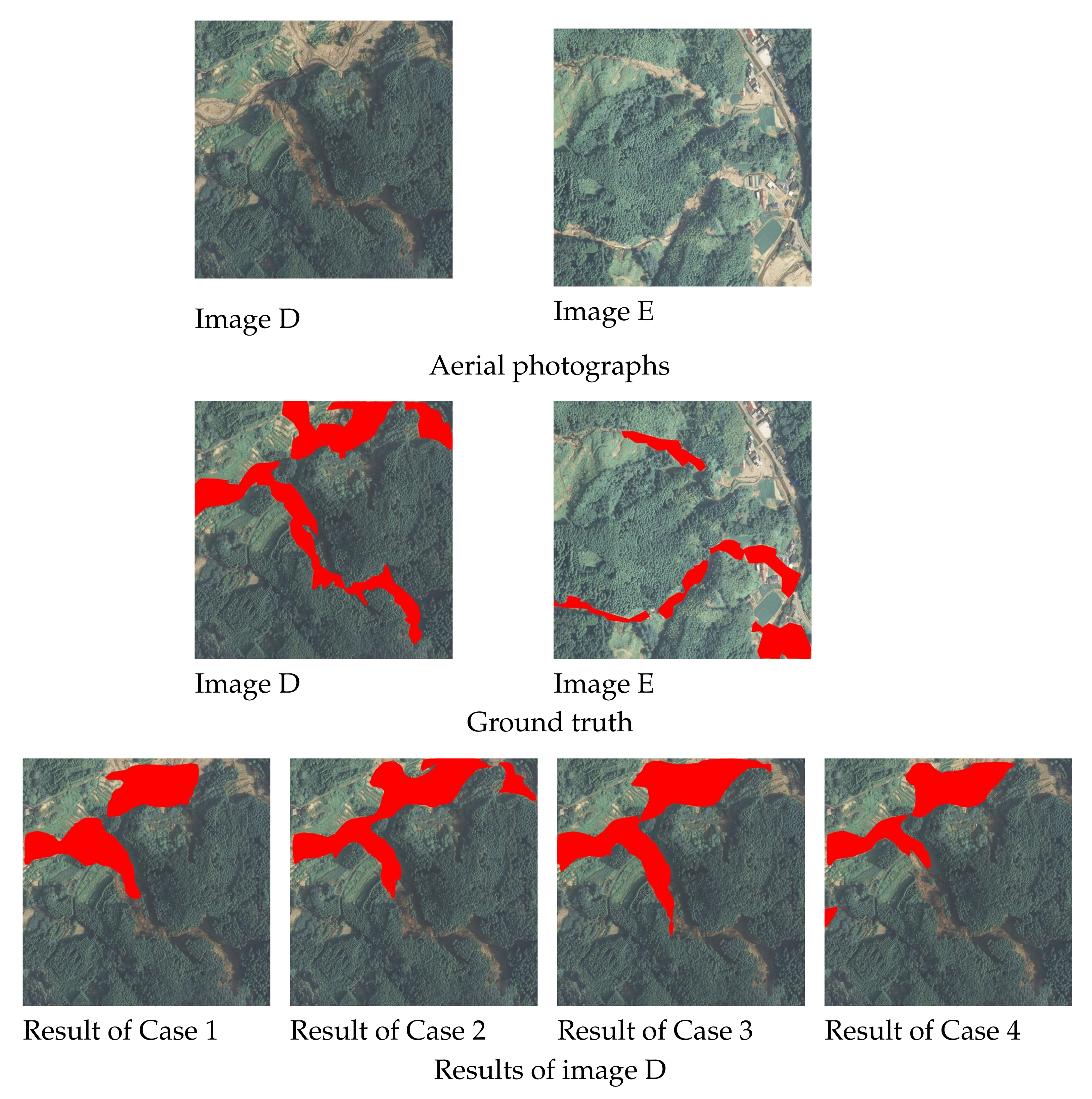
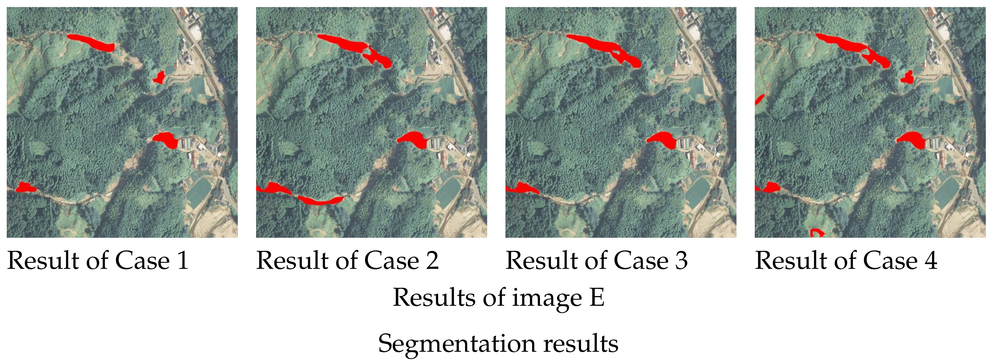
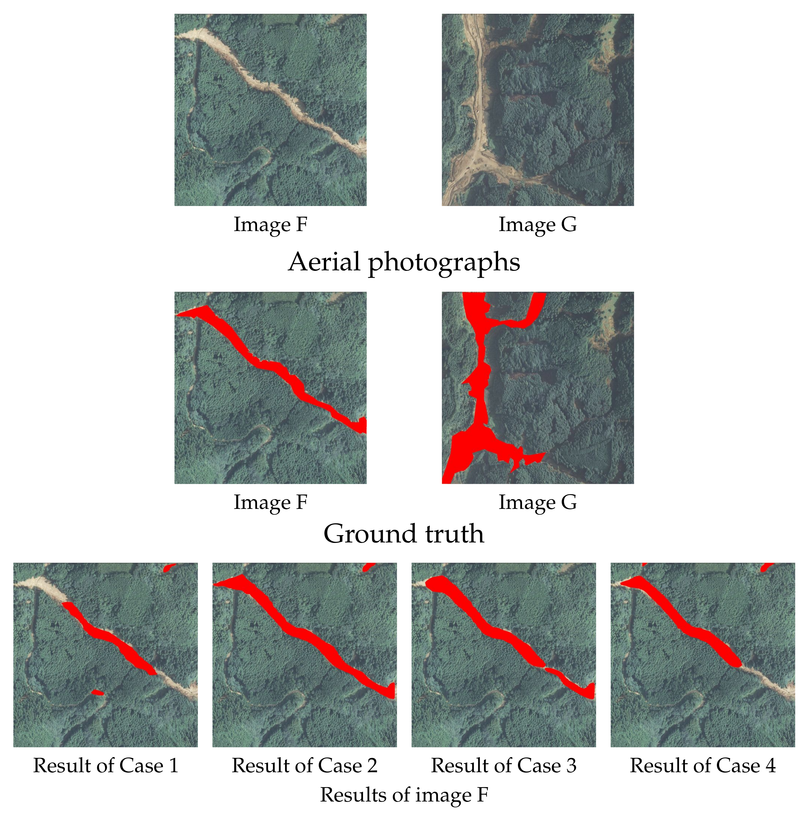
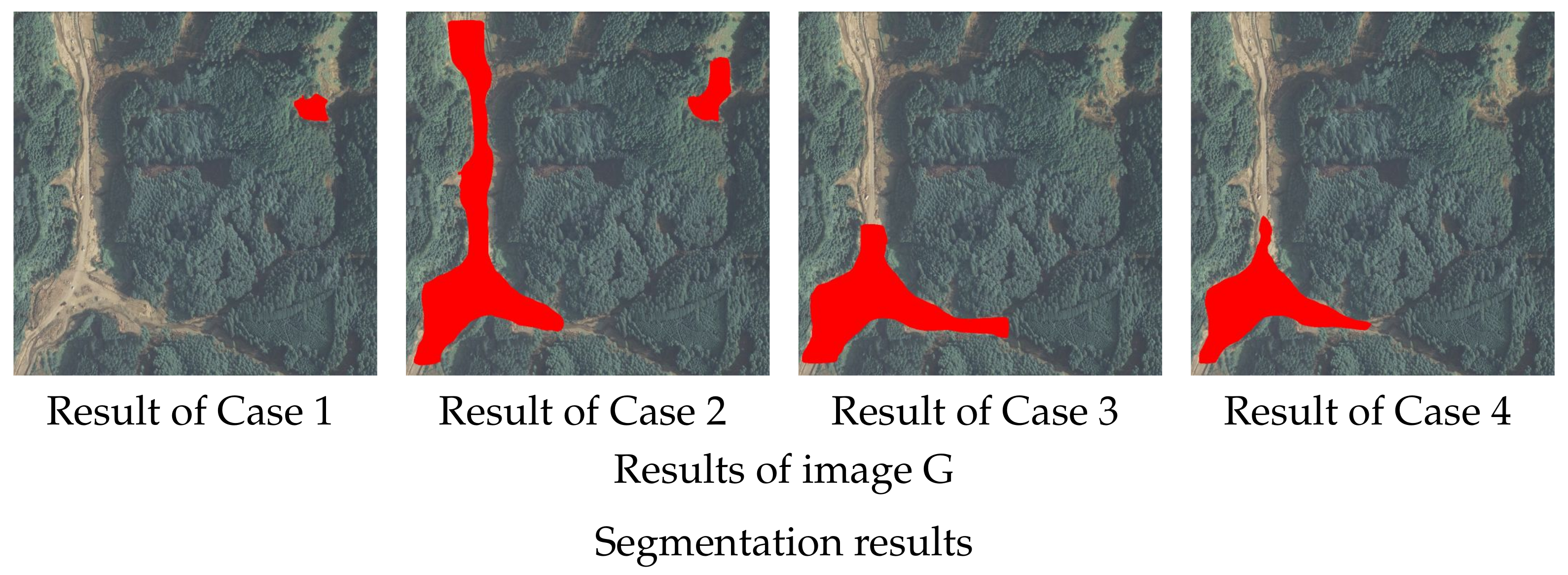
3.1. Results of Slope Failure Detection
3.2. Accuracy Assessment
4. Discussion
5. Conclusions
Author Contributions
Funding
Institutional Review Board Statement
Informed Consent Statement
Data Availability Statement
Conflicts of Interest
References
- Guzzetti, F.; Mondini, A.; Cardinali, M.; Fiorucci, F.; Santangelo, M.; Chang, K. Landslide inventory maps: New tools for an old problem. Earth-Sci. Rev. 2012, 112, 42–66. [Google Scholar] [CrossRef]
- Ghorbanzadeh, O.; Xu, Y.; Ghamisi, P.; Kopp, M.; Kreil, D. Landslide4Sence: Reference Benchmark Data and Deep Learning Models for Landslide Detection. arXiv 2022, arXiv:2206.00515. [Google Scholar]
- Japanese Geotechnical Society: Report of the Emergency Disaster Investigation Team on the Damage Survey in Taiwan Caused by Typhoon Morakot in 2009. 2009. Available online: https://www.jiban.or.jp/file/organi/bu/somubu/Morakot-report.pdf (accessed on 26 July 2022). (In Japanese).
- Chandra, K. Deluge, disaster and development in Uttarakhand Himalayan region of India, Challenges and lessons for disaster management. Int. J. Disaster Risk Reduct. 2014, 8, 143–152. [Google Scholar]
- Osanai, N.; Kaibori, M.; Yamada, T.; Kasai, M.; Hayashi, S.; Katsura, S.; Furuichi, T.; Yanai, S.; Takebayashi, H.; Fujinami, T.; et al. Sediment-related disasters induced by the 2018 Hokkaido Eastern Iburi Earthquake. J. Jpn. Soc. Eros. Control Eng. 2019, 71, 54–65. (In Japanese) [Google Scholar]
- Committee on Hydroscience and Hydraulic Engineering The 2017 Northern Kyushu floods Research Team: The 2017 Northern Kyushu floods research report. 2020. Available online: https://committees.jsce.or.jp/report/system/files/H29%E4%B9%9D%E5%B7%9E%E5%8C%97%E9%83%A8%E8%B1%AA%E9%9B%A8%E7%81%BD%E5%AE%B3%E8%AA%BF%E6%9F%BB%E5%9B%A3_%E5%A0%B1%E5%91%8A%E6%9B%B8.pdf (accessed on 26 July 2022). (In Japanese).
- Hara, T.; Zhang, H.; Sakamoto, J. Reflections on the heavy rain event of July 2018 that struck the Southwest Region of Kochi Prefecture, JSCE Magazine. Civ. Eng. 2020, 105, 68–71. Available online: https://www.jsce.or.jp/journal/jikosaigai/202002.pdf (accessed on 26 July 2022). (In Japanese).
- Afaq, Y.; Manocha, A. Analysis on change detection techniques for remote sensing applications: A review. Ecol. Inform. 2021, 63, 101310. [Google Scholar] [CrossRef]
- Aimaiti, Y.; Liu, W.; Yamazaki, F.; Maruyama, Y. Earthquake-Induced Landslide Mapping for the 2018 Hokkaido Eastern Iburi Earthquake Using PALSAR-2 Data. Remote Sens. 2019, 11, 2351. [Google Scholar] [CrossRef]
- Miura, H.; Midorikawa, S. Detection of Slope Failure Areas due to the 2004 Niigata-ken Chuetsu Earthquake Using High-Resolution Satellite Images and Digital Elevation Model. J. Jpn. Assoc. Earthq. Eng. 2007, 7, 1–14. (In Japanese) [Google Scholar]
- Amit, S.N.K.B.; Aoki, Y. Disaster detection from aerial imagery with convolutional neural network. In Proceedings of the 2017 International Electronics Symposium on Knowledge Creation and Intelligent Computing (IES-KCIC), Surabaya, Indonesia, 26–27 September 2017; pp. 239–245. [Google Scholar]
- Kawamura, K.; Nakamura, Y.; Wakatsuki, T.; Samura, T. A Study on the Automatic Detection of Landslide from Aerial Photographs Using Deep Learning. J. Jpn. Soc. Civ. Eng. 2018, 74, I_132–I_143. (In Japanese) [Google Scholar] [CrossRef]
- Ghorbanzadeh, O.; Blaschke, T.; Gholamnia, K.; Meena, S.R.; Tiede, D.; Aryal, J. Evaluation of Different Machine Learning Methods and Deep-Learning Convolutional Neural Networks for Landslide Detection. Remote Sens. 2019, 11, 196. [Google Scholar] [CrossRef]
- Ghorbanzadeh, O.; Meena, S.R.; Blaschke, T.; Aryal, J. UAV-Based Slope Failure Detection Using Deep-Learning Convolutional Neural Networks. Remote Sens. 2019, 11, 2046. [Google Scholar] [CrossRef]
- Dong, L.; Shan, J. A comprehensive review of earthquake-induced building damage detection with remote sensing techniques. ISPRS J. Photogramm. Remote Sens. 2013, 84, 85–99. [Google Scholar] [CrossRef]
- Ghorbanzadeh, O.; Crivellari, A.; Ghamisi, P.; Shahabi, H.; Blaschke, T. A comprehensive transferability evaluation of U-Net and ResU-Net for landslide detection from Sentinel-2 data (case study areas from Taiwan, China, and Japan). Sci. Rep. 2021, 11, 14629. [Google Scholar] [CrossRef] [PubMed]
- Ghorbanzadeh, O.; Shahabi, H.; Crivellari, A.; Homayouni, S.; Blaschke, T.; Ghamisi, P. Landslide detection using deep learning and object-based image analysis. Landslides 2022, 19, 929–939. [Google Scholar] [CrossRef]
- Oh, Y.; Park, S.; Ye, J. Deep Learning COVID-19 Features on CXR Using Limited Training Data Sets. IEEE Trans. Med Imaging 2020, 39, 2688–2700. [Google Scholar] [CrossRef]
- Shahabi, H.; Rahimzad, M.; Piralilou, S.; Ghorbanzadeh, O.; Homayouni, S.; Blaschke, T.; Lim, S.; Ghamisi, P. Unsupervised Deep Learning for Landslide Detection from Multispectral Sentinel-2 Imagery. Remote Sens. 2021, 13, 46938. [Google Scholar] [CrossRef]
- Kikuchi, T.; Sakita, K.; Hatano, T.; Yoshikawa, K.; Nishiyama, S.; Ohnishi, Y. Automatic differenciation of failure and non failure sites using deep learning. J. Jpn. Landslide Soc. 2019, 56, 255–263. (In Japanese) [Google Scholar] [CrossRef]
- DeVries, T.; Taylor, G.W. Improved Regularization of Convolutional Neural Networks with Cutout. In Proceedings of the 2017 Computer Vision and Pattern Recognition, Honolulu, HI, USA, 21–26 July 2017. [Google Scholar]
- Zhang, H.; Cisse, M.; Dauphin, Y.N.; Lopez-Paz, D. mixup: Beyond Empirical Risk Minimization. In Proceedings of the International Conference on Learning Representations (ICLR), Vancouver, BC, Canada, 30 April–3 May 2018. [Google Scholar]
- Yun, S.; Han, D.; Chun, S.; Oh, S.J.; Yoo, Y.; Choe, J. CutMix: Regularization Strategy to Train Strong Classifiers with Localizable Features. In Proceedings of the 2019 IEEE/CVF International Conference on Computer Vision (ICCV), Seoul, Korea, 27 October–2 November 2019; pp. 6022–6031. [Google Scholar]
- Chun, P.J.; Izumi, S.; Yamane, T. Automatic detection method of cracks from concrete surface imagery using two-step Light Gradient Boosting Machine. Comput.-Aided Civ. Infrastruct. Eng. 2020, 36, 61–72. [Google Scholar] [CrossRef]
- Yamane, T.; Chun, P.J. Crack detection from a concrete surface image based on semantic segmentation using deep learning. Adv. Concr. Technol. 2020, 18, 493–504. [Google Scholar] [CrossRef]
- Yamane, T.; Chun, P.J.; Honda, R. Detecting and Localising Damage Based on Image Recognition and Structure from Motion, and Reflecting it in a 3D Bridge Model. Struct. Infrastruct. Eng. 2022; in print. [Google Scholar]
- Opara, J.; Thein, A.; Izumi, S.; Yasuhara, H.; Chun, P.J. Defect Detection on Asphalt Pavement by Deep Learning. Int. J. GEOMATE 2021, 21, 87–94. [Google Scholar] [CrossRef]
- Chun, P.J.; Yamane, T.; Tsuzuki, Y. Automatic Detection of Cracks in Asphalt Pavement Using Deep Learning to Overcome Weaknesses in Images and GIS Visualization. Appl. Sci. 2021, 11, 892. [Google Scholar] [CrossRef]
- Chun, P.J.; Dang, J.; Hamasaki, S.; Yajima, R.; Kameda, T.; Wada, H.; Yamane, T.; Izumi, S.; Nagatani, K. Utilization of Unmanned Aerial Vehicle, Artificial Intelligence, and Remote Measurement Technology for Bridge Inspections. J. Robot. Mechatronics 2020, 32, 1244–1258. [Google Scholar] [CrossRef]
- Chun, P.J.; Funatani, K.; Furukawa, S.; Ohga, M. Grade Classification of Corrosion Damage on The Surface of Weathering Steel Members by Digital Image Processing. In Proceedings of the Thirteenth East Asia-Pacific Conference on Structural Engineering and Construction, Sapporo, Japan, 11–13 September 2013. [Google Scholar]
- Chun, P.J.; Yamane, T.; Izumi, S.; Kameda, T. Evaluation of tensile performance of steel members by analysis of corroded steel surface using deep learning. Metals 2019, 9, 1259. [Google Scholar] [CrossRef]
- Karina, C.N.; Chun, P.J.; Okubo, K. Tensile strength prediction of corroded steel plates by using machine learning approach. Steel Compos. Struct 2017, 24, 635–641. [Google Scholar]
- Chun, P.J.; Yamane, T.; Maemura, Y. A deep learning based image captioning method to automatically generate comprehensive explanations of bridge damage. Comput.-Aided Civ. Eng. Infrastruct. Eng. 2021, 37, 1387–1401. [Google Scholar] [CrossRef]
- Moon, H.S.; Ok, S.; Chun, P.J.; Lim, Y.M. Artificial neural network for vertical displacement prediction of a bridge from strains (Part 1): Girder bridge under moving vehicles. Appl. Sci. 2019, 9, 2881. [Google Scholar] [CrossRef] [Green Version]
- Xu, H.; Su, X.; Wang, Y.; Cai, H.; Cui, K.; Chen, X. Automatic Bridge Crack Detection Using a Convolutional Neural Network. Appl. Sci. 2019, 9, 2867. [Google Scholar] [CrossRef]
- Bang, S.; Park, H.; Kim, H.; Kim, H. Encoder-decoder network for pixel-level road crack detection in black-box images. Comput.-Aided Civ. Infrastruct. Eng. 2019, 34, 713–727. [Google Scholar] [CrossRef]
- Girshick, R.; Donahue, J.; Darrell, T.; Malik, J. Rich Feature Hierarchies for Accurate Object Detection and Semantic Segmentation. In Proceedings of the 2014 IEEE Conference on Computer Vision and Pattern Recognition, Columbus, OH, USA, 23–28 June 2014; pp. 580–587. [Google Scholar]
- He, K.; Gkioxari, G.; Dollar, P.; Girshick, R. Mask R-CNN. In Proceedings of the 2017 IEEE International Conference on Computer Vision (ICCV), Venice, Italy, 22–29 October 2017; pp. 2980–2988. [Google Scholar]
- Girshick, R. Fast R-CNN. In Proceedings of the IEEE International Conference on Computer Vision (ICCV), Santiago, Chile, 7–13 December 2015; pp. 1440–1448. [Google Scholar]
- Ren, S.; He, K.; Girshick, R.; Sun, J. Faster R-CNN: Towards Real-Time Object Detection with Region Proposal Networks. IEEE Trans. Pattern Anal. Mach. Intell. 2017, 39, 1137–1149. [Google Scholar] [CrossRef] [Green Version]
- He, K.; Zhang, X.; Ren, S.; Sun, J. Spatial Pyramid Pooling in Deep Convolutional Networks for Visual Recognition. Eur. Conf. Comput. Vis. (EVVC 2014) 2014, 8691, 346–361. [Google Scholar]
- Geospatial Information Authority of Japan. GIS Maps. Available online: https://maps.gsi.go.jp/ (accessed on 26 July 2022). (In Japanese).
- Kanai, K.; Yamane, T.; Ishiguro, S.; Chun, P.J. Automatic Detection of Slope Failure Regions Using Semantic Segmentation. Intell. Inform. Infrastruct. 2020, 1, 421–428. (In Japanese) [Google Scholar]


| Training Data | Validation Data | Test Data | ||
|---|---|---|---|---|
| Images | Augmentation | |||
| Case 1 | 591 images | No | 197 images | 145 images |
| Case 2 | 12,411 images | One time cutmix | ||
| Case 3 | Two times cutmix | |||
| Case 4 | One time cutmix, rotation, warping | |||
| Value/Number of Epoch | |
|---|---|
| Case 1 | 1.621/ 32 |
| Case 2 | 1.129/178 |
| Case 3 | 1.200/132 |
| Case 4 | 1.255/152 |
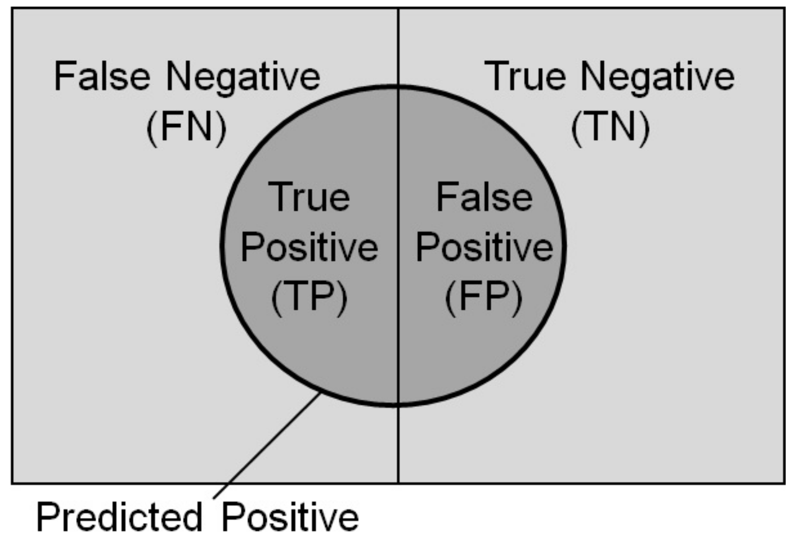
| True Class | Slope Failure Regions | Non-Slope Failure Regions | |
|---|---|---|---|
| Prediction Class | |||
| Slope failure regions | TP (True Positive) | FP (False Positive) | |
| Non-slope failure regions | FN (False Negative) | TN (True Negative) | |
| True Class | Slope Failure Regions | Non-Slope Failure Regions | |
|---|---|---|---|
| Prediction Class | |||
| Slope failure regions | Case 1 | 6,527,912 | 2,518,387 |
| Case 2 | 8,891,079 | 2,447,233 | |
| Case 3 | 8,650,994 | 3,175,846 | |
| Case 4 | 6,865,760 | 1,603,504 | |
| Non-slope failure regions | Case 1 | 6,153,051 | 136,844,170 |
| Case 2 | 3,789,884 | 136,915,324 | |
| Case 3 | 4,029,969 | 136,186,711 | |
| Case 4 | 5,815,203 | 137,759,053 |
| Case 1 | Case 2 | Case 3 | Case 4 | |
|---|---|---|---|---|
| Accuracy | 0.943 | 0.959 | 0.953 | 0.951 |
| Precision | 0.722 | 0.784 | 0.731 | 0.811 |
| Recall | 0.515 | 0.701 | 0.682 | 0.541 |
| Specificity | 0.982 | 0.982 | 0.977 | 0.988 |
| F1 score | 0.601 | 0.740 | 0.706 | 0.649 |
Publisher’s Note: MDPI stays neutral with regard to jurisdictional claims in published maps and institutional affiliations. |
© 2022 by the authors. Licensee MDPI, Basel, Switzerland. This article is an open access article distributed under the terms and conditions of the Creative Commons Attribution (CC BY) license (https://creativecommons.org/licenses/by/4.0/).
Share and Cite
Kubo, S.; Yamane, T.; Chun, P.-j. Study on Accuracy Improvement of Slope Failure Region Detection Using Mask R-CNN with Augmentation Method. Sensors 2022, 22, 6412. https://doi.org/10.3390/s22176412
Kubo S, Yamane T, Chun P-j. Study on Accuracy Improvement of Slope Failure Region Detection Using Mask R-CNN with Augmentation Method. Sensors. 2022; 22(17):6412. https://doi.org/10.3390/s22176412
Chicago/Turabian StyleKubo, Shiori, Tatsuro Yamane, and Pang-jo Chun. 2022. "Study on Accuracy Improvement of Slope Failure Region Detection Using Mask R-CNN with Augmentation Method" Sensors 22, no. 17: 6412. https://doi.org/10.3390/s22176412
APA StyleKubo, S., Yamane, T., & Chun, P.-j. (2022). Study on Accuracy Improvement of Slope Failure Region Detection Using Mask R-CNN with Augmentation Method. Sensors, 22(17), 6412. https://doi.org/10.3390/s22176412