
An Improved Circular Fringe Fourier Transform Profilometry


Abstract
:1. Introduction
2. Principle
2.1. Geometric Model and Calculation of Lateral Displacement of CFFTP
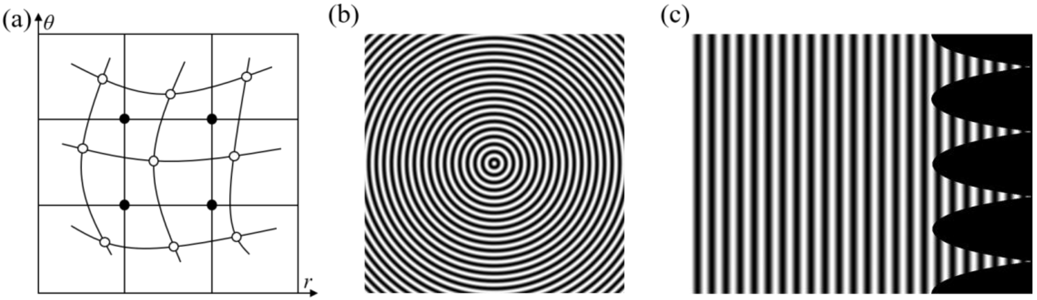
2.2. Coordinate Transformation of CFFTP
2.3. Calculation of Conical Phase by FTP
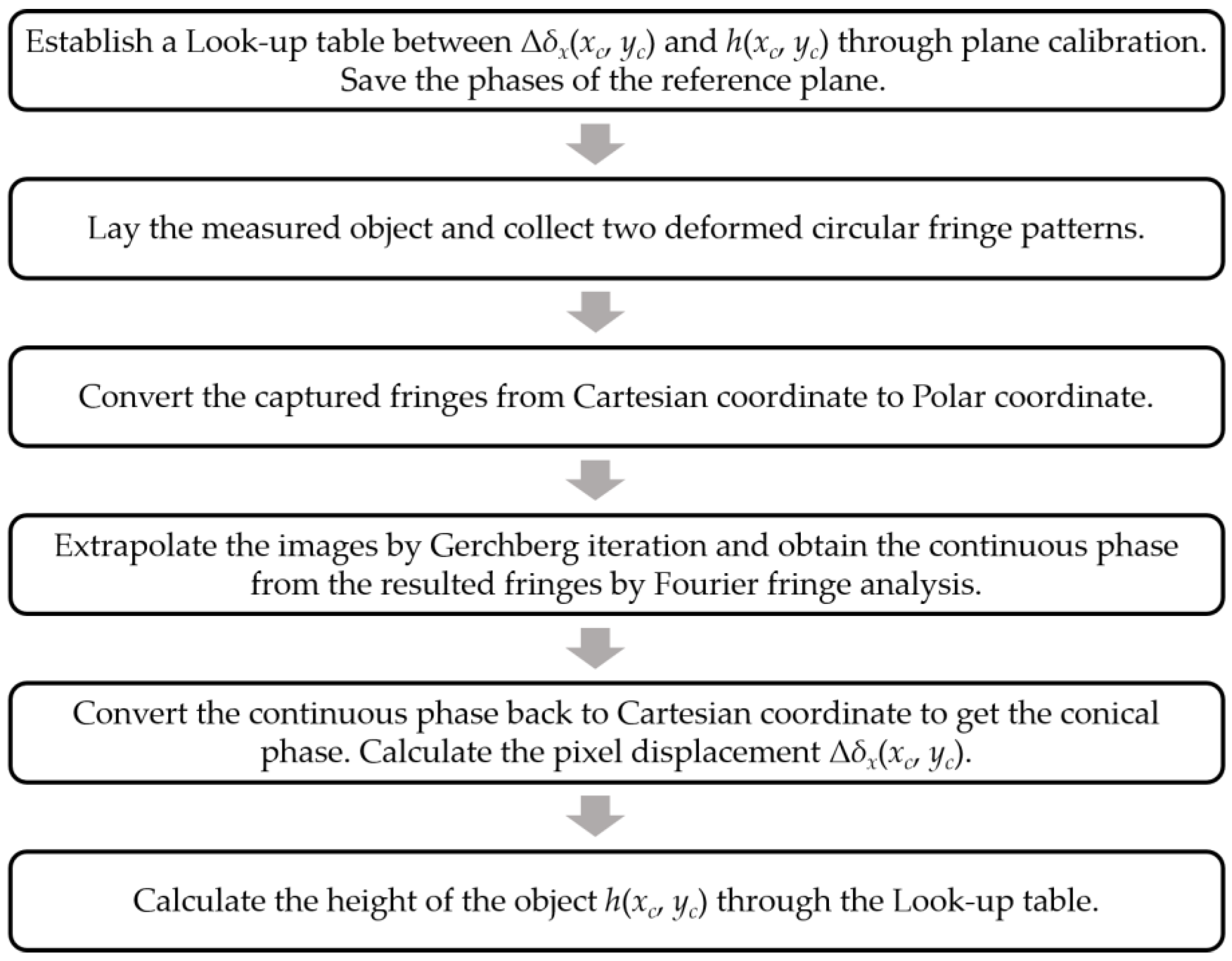
2.4. Establishment of the Displacement-to-Height Mapping
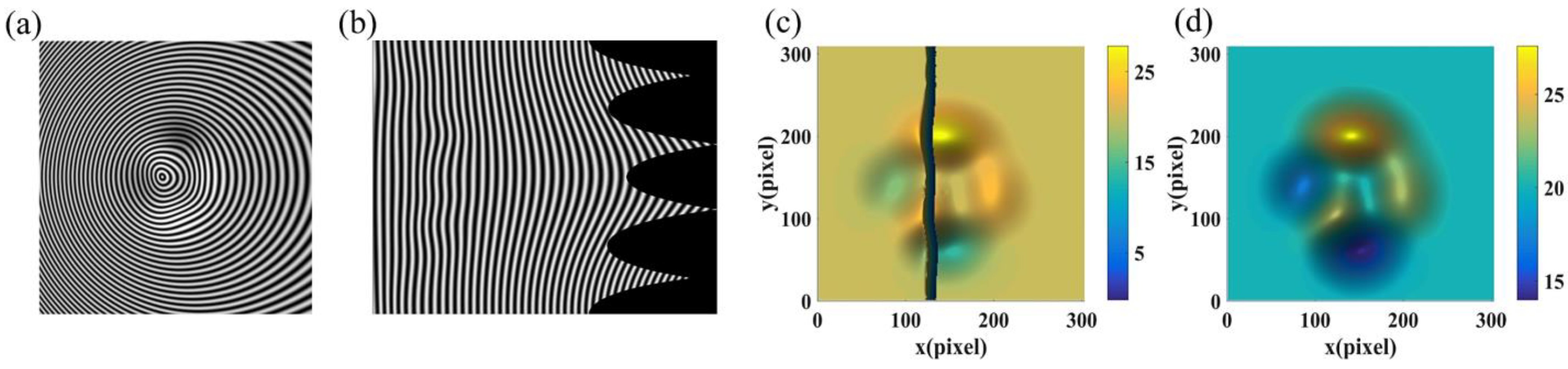
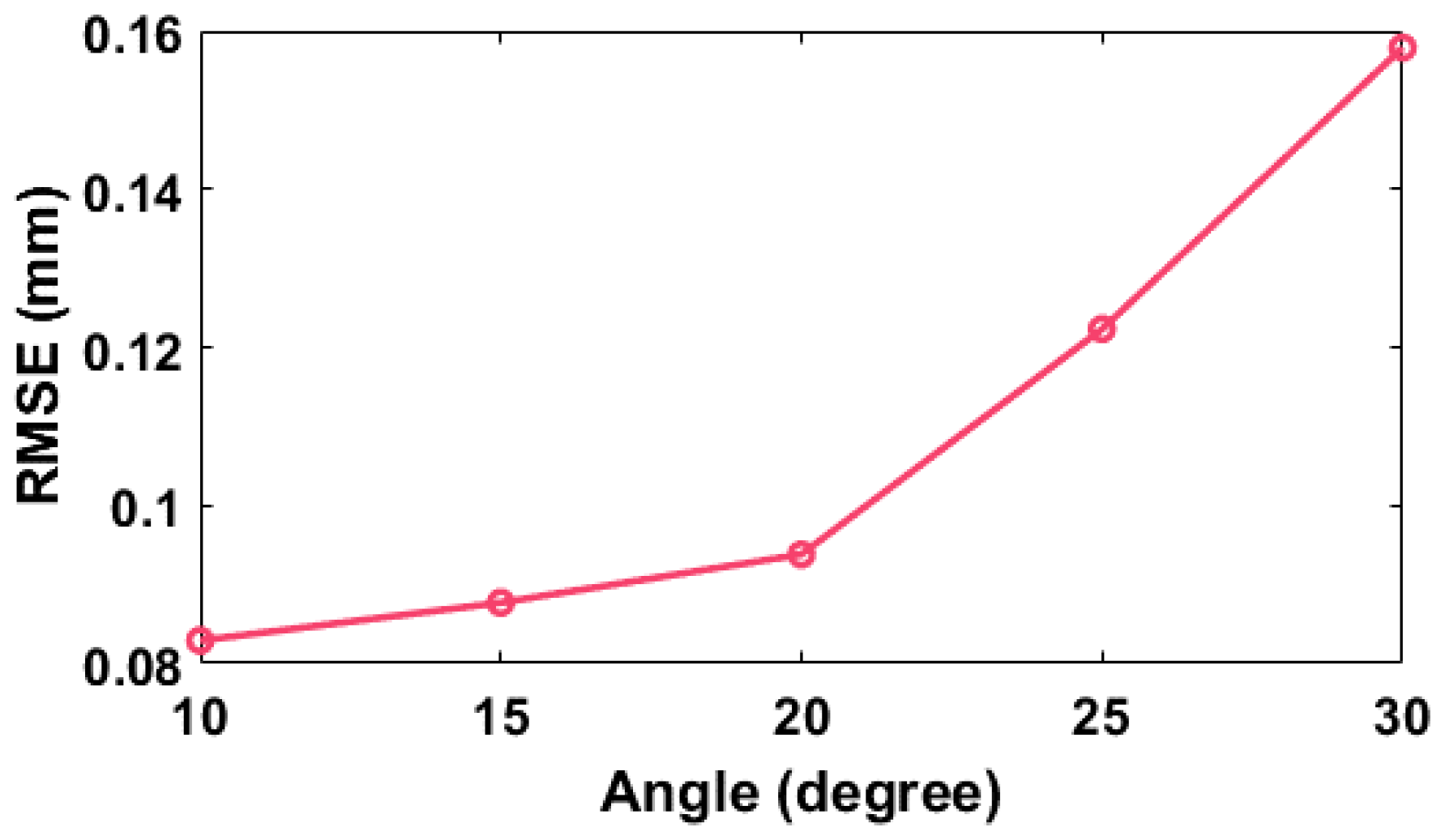
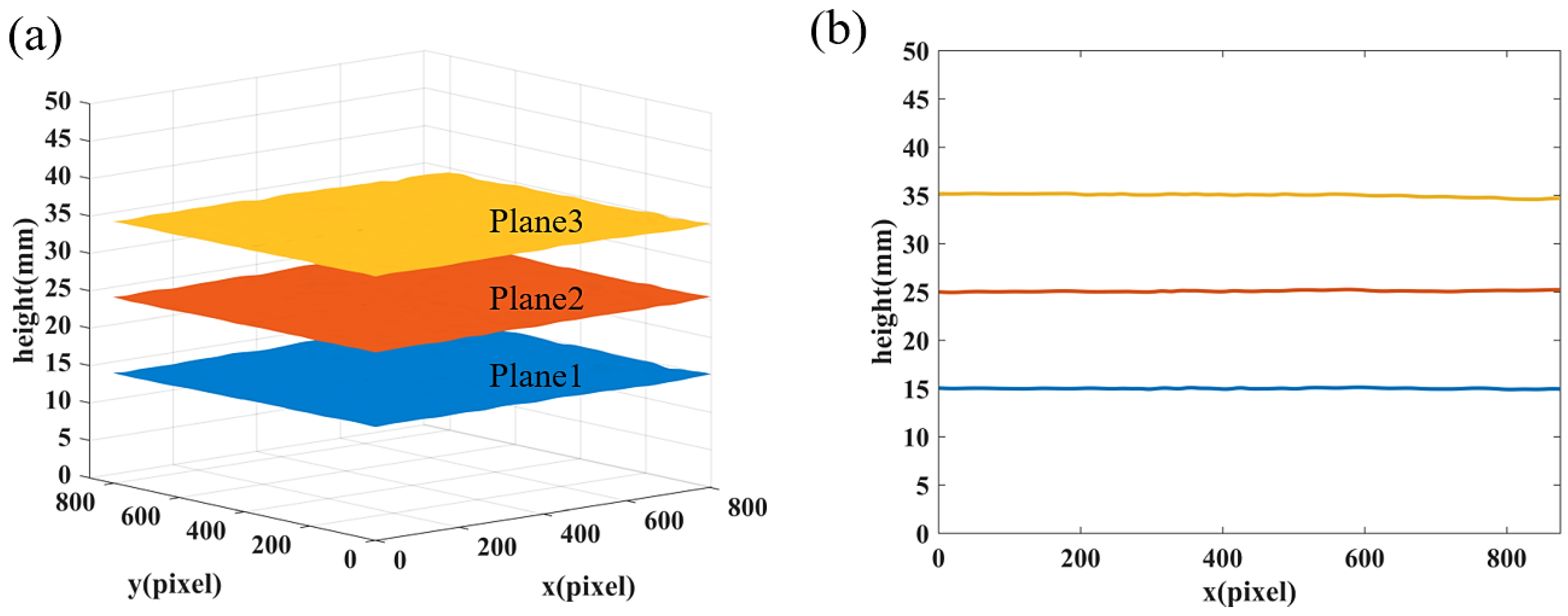
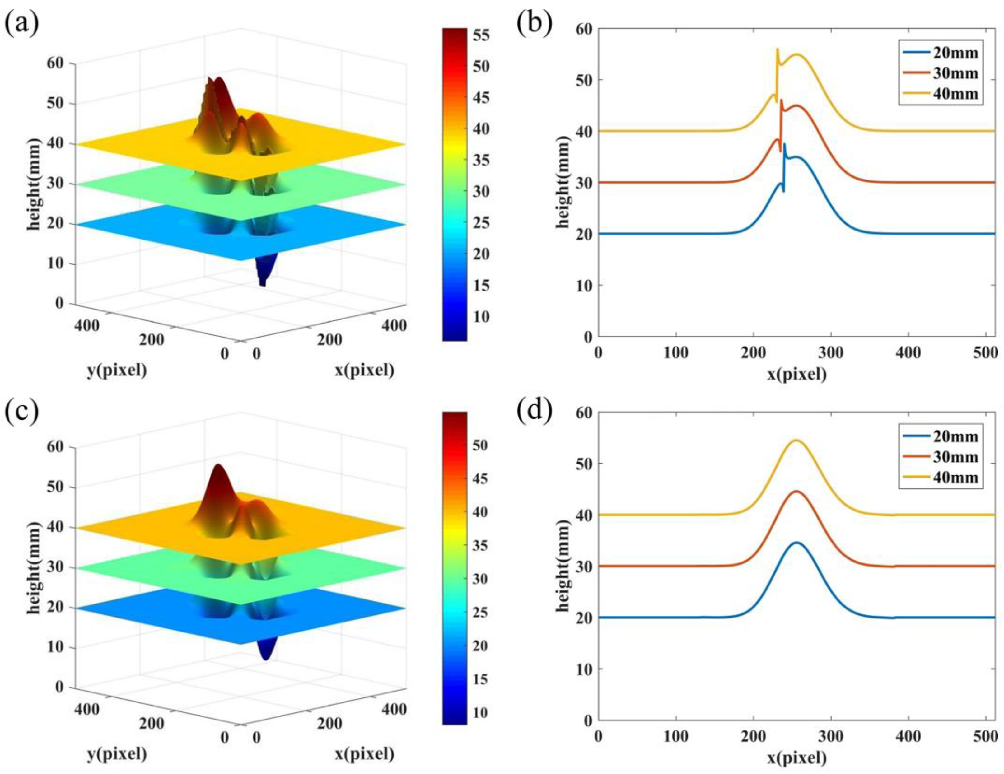
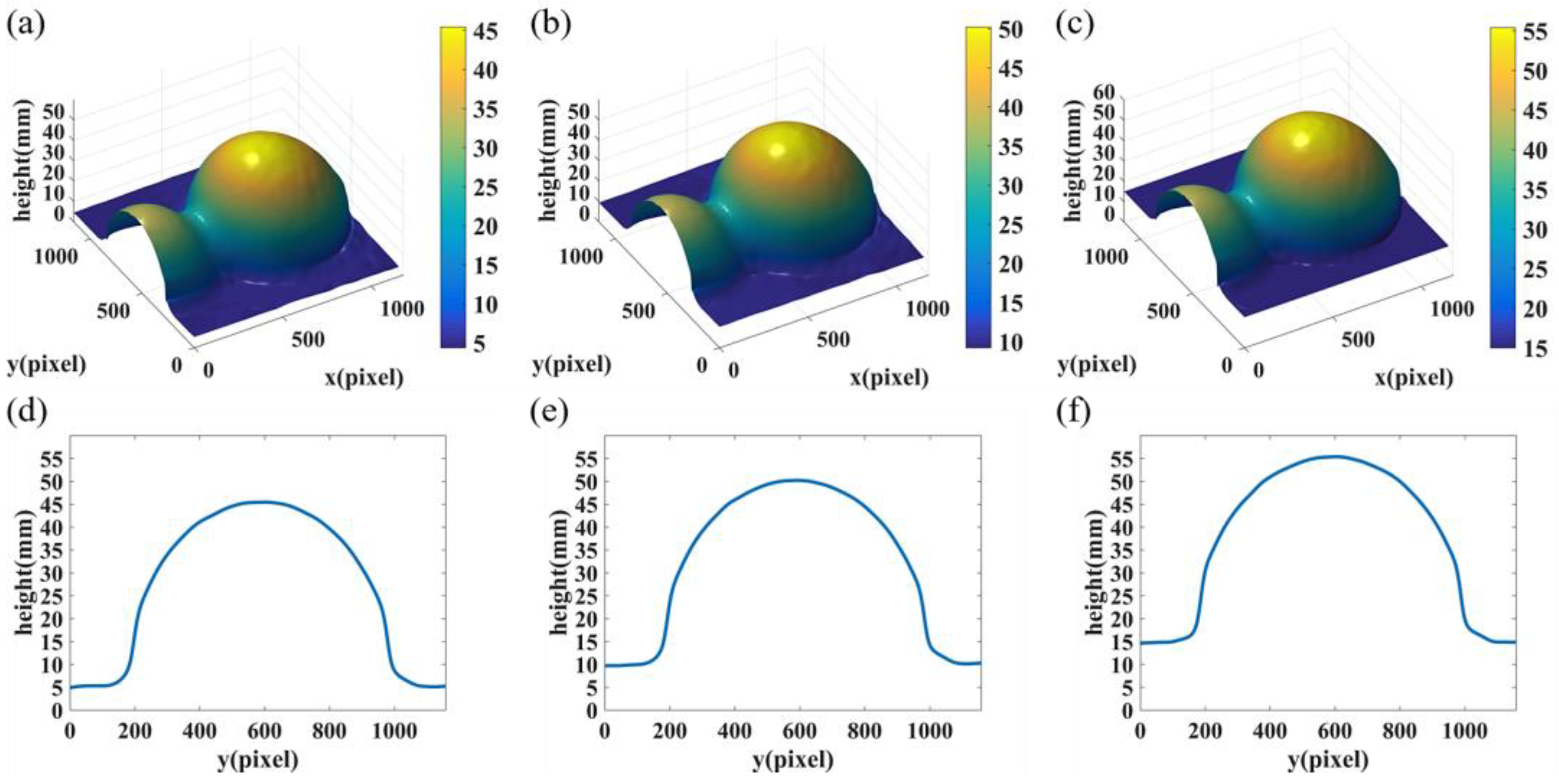
3. Simulations
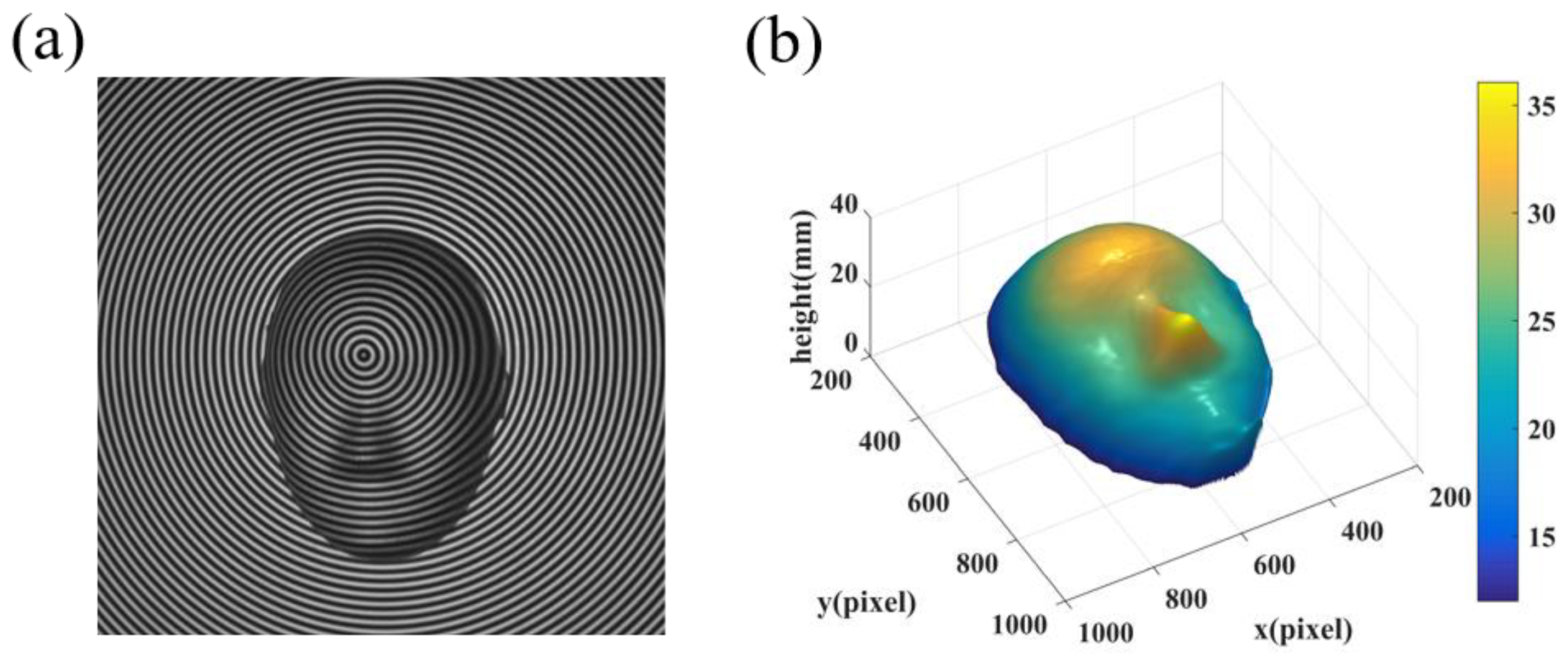
4. Experiments
5. Conclusions
Author Contributions
Funding
Institutional Review Board Statement
Informed Consent Statement
Data Availability Statement
Conflicts of Interest
References
- Chen, F.; Brown, G.; Song, M. Overview of three-dimensional shape measurement using optical methods. Opt. Eng. 2000, 39, 10–22. [Google Scholar]
- Zuo, C.; Feng, S.; Huang, L.; Tao, T.; Yin, W.; Chen, Q. Phase shifting algorithms for fringe projection profilometry: A review. Opt. Lasers Eng. 2018, 109, 23–59. [Google Scholar] [CrossRef]
- Su, X.; Chen, W. Fourier transform profilometry: A review. Opt. Lasers Eng. 2001, 35, 263–284. [Google Scholar] [CrossRef]
- Geng, J. Structured-light 3D surface imaging: A tutorial. Adv. Opt. Photon. 2011, 3, 128–160. [Google Scholar] [CrossRef]
- Gorthi, S.; Rastogi, P. Fringe projection techniques: Whither we are? Opt. Lasers Eng. 2010, 48, 133–140. [Google Scholar] [CrossRef]
- Kulkarni, R.; Banoth, E.; Pal, P. Automated surface feature detection using fringe projection: An autoregressive modeling-based approach. Opt. Lasers Eng. 2019, 121, 506–511. [Google Scholar] [CrossRef]
- Chen, L.; Quan, C.; Tay, C.; Yu, F. Shape measurement using one frame projected sawtooth fringe pattern. Opt. Commun. 2005, 246, 275–284. [Google Scholar] [CrossRef]
- Jia, P.; Kofman, J.; English, C. Error compensation in two-step triangular-pattern phase-shifting profilometry. Opt. Lasers Eng. 2008, 46, 311–320. [Google Scholar] [CrossRef]
- Iwata, K.; Kusunoki, F.; Moriwaki, K.; Fukuda, H.; Tomii, T. Three-dimensional profiling using the Fourier transform method with a hexagonal grating projection. Appl. Opt. 2008, 47, 2103–2108. [Google Scholar] [CrossRef]
- Zhang, C.; Zhao, H.; Qiao, J.; Zhou, C.; Zhang, L.; Hu, G.; Geng, H. Three-dimensional measurement based on optimized circular fringe projection technique. Opt. Express 2019, 27, 2465–2477. [Google Scholar] [CrossRef] [PubMed]
- Ma, Y.; Yin, D.; Wei, C.; Feng, S.; Ma, J.; Nie, S.; Yuan, C. Real-time 3-D shape measurement based on radial spatial carrier phase shifting from circular fringe pattern. Opt. Commun. 2019, 450, 6–13. [Google Scholar] [CrossRef]
- Zuo, C.; Tao, T.; Feng, S.; Huang, L.; Asundi, A.; Chen, Q. Micro Fourier transform profilometry (μFTP): 3D shape measurement at 10,000 frames per second. Opt. Lasers Eng. 2018, 102, 70–91. [Google Scholar] [CrossRef]
- Li, B.; An, Y.; Zhang, S. Single-shot absolute 3D shape measurement with Fourier transform profilometry. Appl. Opt. 2016, 55, 5219–5225. [Google Scholar] [CrossRef] [PubMed]
- Wang, Z.; Zhang, Z.; Gao, N.; Xiao, Y.; Gao, F.; Jiang, X. Single-shot 3D shape measurement of discontinuous objects based on a coaxial fringe projection system. Appl. Opt. 2019, 58, A169–A178. [Google Scholar] [CrossRef] [PubMed]
- Su, W.; Liu, Z. Fourier-transform profilometry using a pulse-encoded fringe pattern. In Proceedings of the SPIE Optical Engineering + Applications, San Diego, CA, USA, 9 September 2019. [Google Scholar]
- Zhang, Z.; Zhong, J. Applicability analysis of wavelet-transform profilometry. Opt. Express 2013, 21, 18777–18796. [Google Scholar] [CrossRef]
- Han, M.; Chen, W. Dual-Angle rotation two-dimensional wavelet transform profilometry. Opt. Lett. 2022, 47, 1395–1398. [Google Scholar] [CrossRef]
- Zheng, S.; Chen, W.; Su, X. Adaptive windowed Fourier transform in 3-D shape measurement. Opt. Eng. 2006, 45, 063601. [Google Scholar] [CrossRef]
- Zhang, Z.; Jing, Z.; Wang, Z.; Kuang, D. Comparison of Fourier transform, windowed Fourier transform, and wavelet transform methods for phase calculation at discontinuities in fringe projection profilometry. Opt. Lasers Eng. 2012, 50, 1152–1160. [Google Scholar] [CrossRef]
- Qian, K. Carrier fringe pattern analysis: Links between methods. Opt. Lasers Eng. 2022, 150, 106874. [Google Scholar]
- Su, X.; Chen, W. Reliability-guided phase unwrapping algorithm: A review. Opt. Lasers Eng. 2004, 42, 245–261. [Google Scholar] [CrossRef]
- Zhang, J.; Tian, X.; Shao, J.; Luo, H.; Liang, R. Phase unwrapping in optical metrology via denoised and convolutional segmentation networks. Opt. Express 2019, 27, 14903–14912. [Google Scholar] [CrossRef] [PubMed]
- Zuo, C.; Huang, L.; Zhang, M.; Chen, Q.; Asundi, A. Temporal phase unwrapping algorithms for fringe projection profilometry: A comparative review. Opt. Lasers Eng. 2016, 85, 84–103. [Google Scholar] [CrossRef]
- Wang, X.; Fua, H.; Ma, J.; Fan, J.; Zhang, X. Three-dimensional reconstruction based on tri-frequency heterodyne principle. In Proceedings of the 10th International Conference of Information and Communication Technology, Wuhan, China, 13–15 November 2020. [Google Scholar]
- Ratnam, M.; Saxena, M.; Gorthi, S. Circular fringe projection technique for out-of-plane deformation measurements. Opt. Lasers Eng. 2019, 121, 369–376. [Google Scholar] [CrossRef]
- Mandapalli, J.; Gorthi, S.; Gorthi, R.; Gorthi, S. Circular Fringe Projection Method for 3D Profiling of High Dynamic Range Objects. In Proceedings of the 14th International Conference on Computer Vision Theory and Applications, Prague, Czech Republic, 1 January 2019. [Google Scholar]
- Zhao, H.; Zhang, C.; Zhou, C.; Jiang, K.; Fang, M. Circular fringe projection profilometry. Opt. Lett. 2016, 41, 4951–4954. [Google Scholar] [CrossRef] [PubMed]
- Wang, N.; Jiang, W.; Zhang, Y. Deep learning–based moiré-fringe alignment with circular gratings for lithography. Opt. Lett. 2021, 46, 1113–1116. [Google Scholar] [CrossRef]
- Khonina, S.; Khorin, P.; Serafimovich, P.; Dzyuba, A.; Georgieva, A.; Petrov, N. Analysis of the wavefront aberrations based on neural networks processing of the interferograms with a conical reference beam. Appl. Phys. B 2022, 128, 60. [Google Scholar] [CrossRef]
- Han, D. Comparison of commonly used image interpolation methods. In Proceedings of the 2nd International Conference on Computer Science and Electronics Engineering, Hangzhou, China, 22–23 March 2013. [Google Scholar]
- Hong, S.; Wang, L.; Truong, T. An improved approach to the cubic-spline interpolation. In Proceedings of the 25th IEEE International Conference on Image Processing, Athens, Greece, 7–10 October 2018. [Google Scholar]
- Ning, L.; Luo, K. An Interpolation Based on Cubic Interpolation Algorithm. In Proceedings of the International Conference 2007 on Information Computing and Automation, Chengdu, China, 14–17 December 2007. [Google Scholar]
- Gerchberg, R. Super-Resolution through Error Energy Reduction. Opt. Acta 1974, 21, 709–720. [Google Scholar] [CrossRef]
- Zhao, W.; Su, X.; Chen, W. Discussion on accurate phase–height mapping in fringe projection profilometry. Opt. Eng. 2017, 56, 104109. [Google Scholar] [CrossRef]
- Zhao, W.; Su, X.; Chen, W. Whole-field high precision point to point calibration method. Opt. Lasers Eng. 2018, 111, 71–79. [Google Scholar] [CrossRef]
- Su, X.; Xue, L. Phase unwrapping algorithm based on fringe frequency analysis in Fourier-transform profilometry. Opt. Eng. 2001, 40, 637–643. [Google Scholar] [CrossRef]
- Liao, R.; Yang, L.; Ma, L.; Yang, J.; Zhu, J. A Dense 3-D Point Cloud Measurement Based on 1-D Background-Normalized Fourier Transform. IEEE Trans. Instrum. Meas. 2021, 70, 5014412. [Google Scholar] [CrossRef]


| Method | Position | ||
|---|---|---|---|
| 20 | 30 | 40 | |
| Existing CFFTP | 0.1875 | 0.2038 | 0.2198 |
| Improved CFFTP | 0.0623 | 0.0746 | 0.0874 |
| Height | Mean | RMSE |
|---|---|---|
| 15.0000 | 14.9683 | 0.1183 |
| 25.0000 | 25.0570 | 0.1227 |
| 35.0000 | 35.0328 | 0.1443 |
Publisher’s Note: MDPI stays neutral with regard to jurisdictional claims in published maps and institutional affiliations. |
© 2022 by the authors. Licensee MDPI, Basel, Switzerland. This article is an open access article distributed under the terms and conditions of the Creative Commons Attribution (CC BY) license (https://creativecommons.org/licenses/by/4.0/).
Share and Cite
Chen, Q.; Han, M.; Wang, Y.; Chen, W. An Improved Circular Fringe Fourier Transform Profilometry. Sensors 2022, 22, 6048. https://doi.org/10.3390/s22166048
Chen Q, Han M, Wang Y, Chen W. An Improved Circular Fringe Fourier Transform Profilometry. Sensors. 2022; 22(16):6048. https://doi.org/10.3390/s22166048
Chicago/Turabian StyleChen, Qili, Mengqi Han, Ye Wang, and Wenjing Chen. 2022. "An Improved Circular Fringe Fourier Transform Profilometry" Sensors 22, no. 16: 6048. https://doi.org/10.3390/s22166048
APA StyleChen, Q., Han, M., Wang, Y., & Chen, W. (2022). An Improved Circular Fringe Fourier Transform Profilometry. Sensors, 22(16), 6048. https://doi.org/10.3390/s22166048