
Sea Cucumber Detection Algorithm Based on Deep Learning


Abstract
:1. Introduction
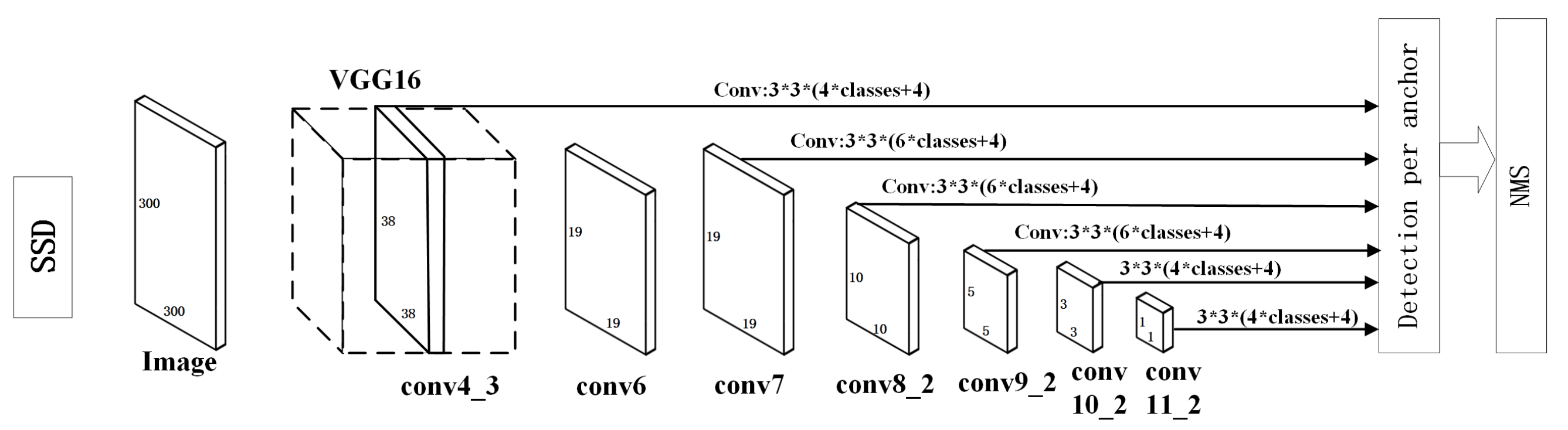
2. SSD Object Detection Algorithm
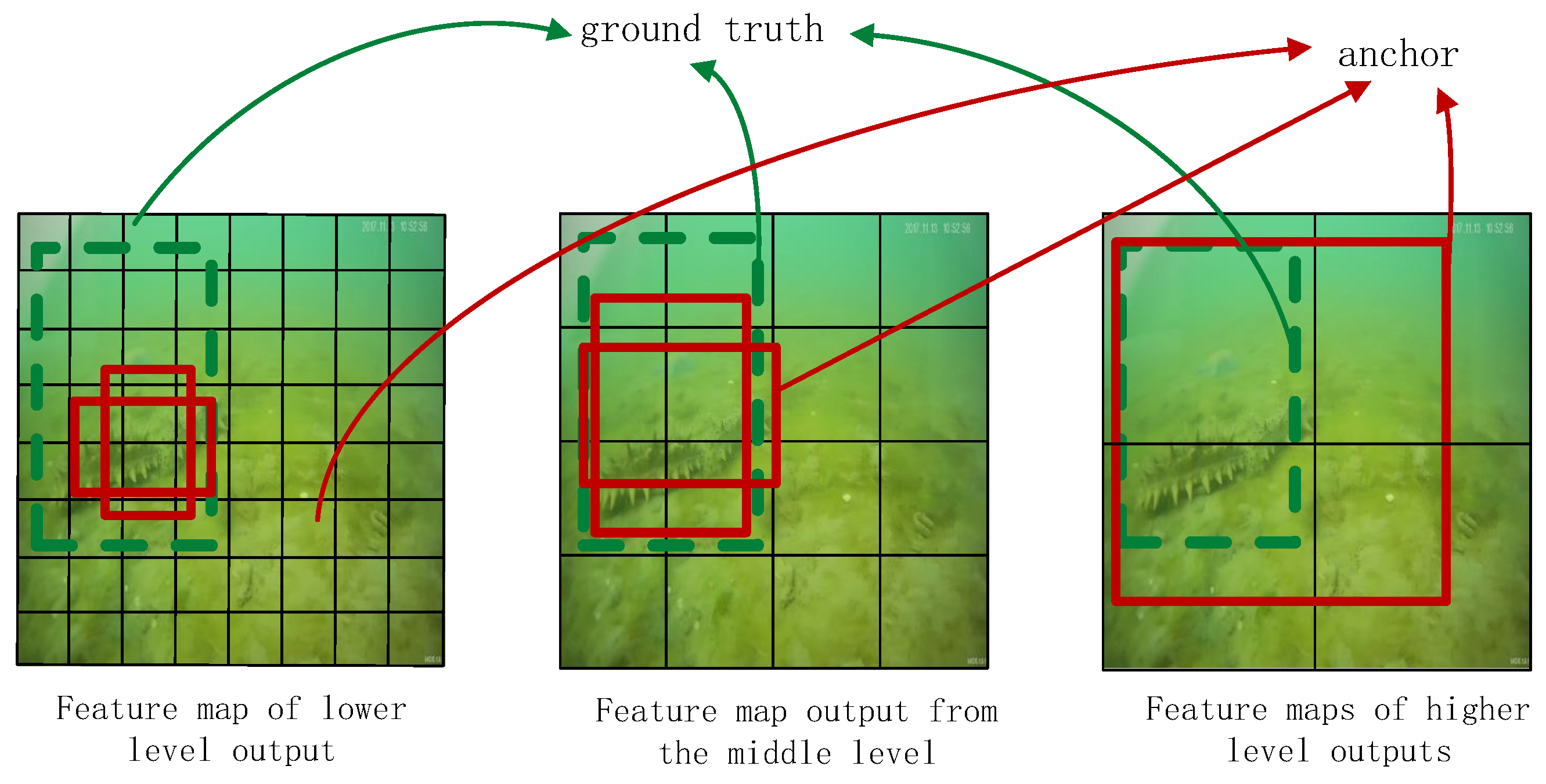
2.1. Traditional SSD Model Structure
2.2. The Loss Function of Traditional SSD
2.3. Traditional SSD Performance Analysis
3. Sea Cucumber Detection Algorithm Based on Improved MobileNetv1 SSD
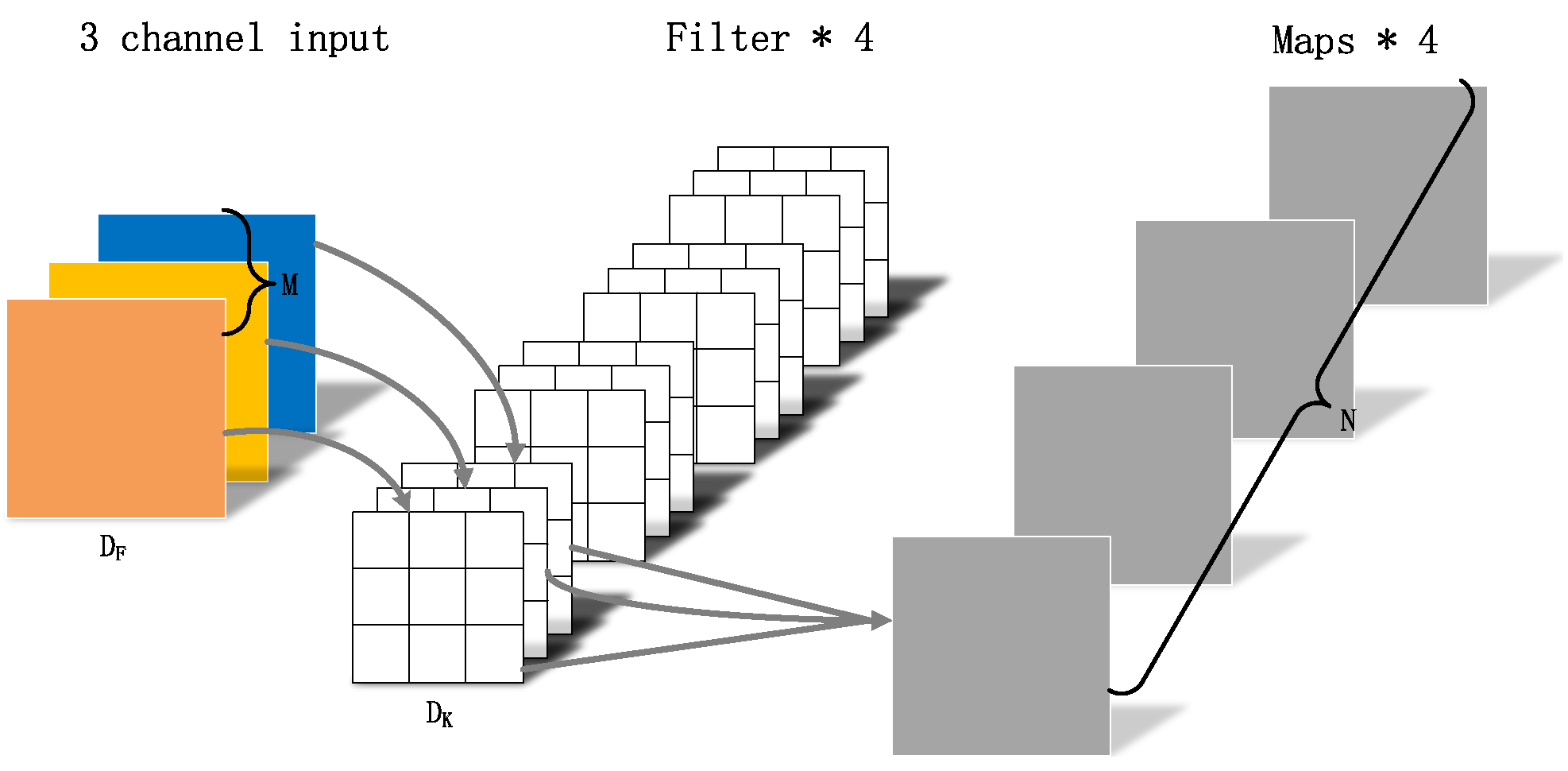
3.1. MobileNetv1 Structure
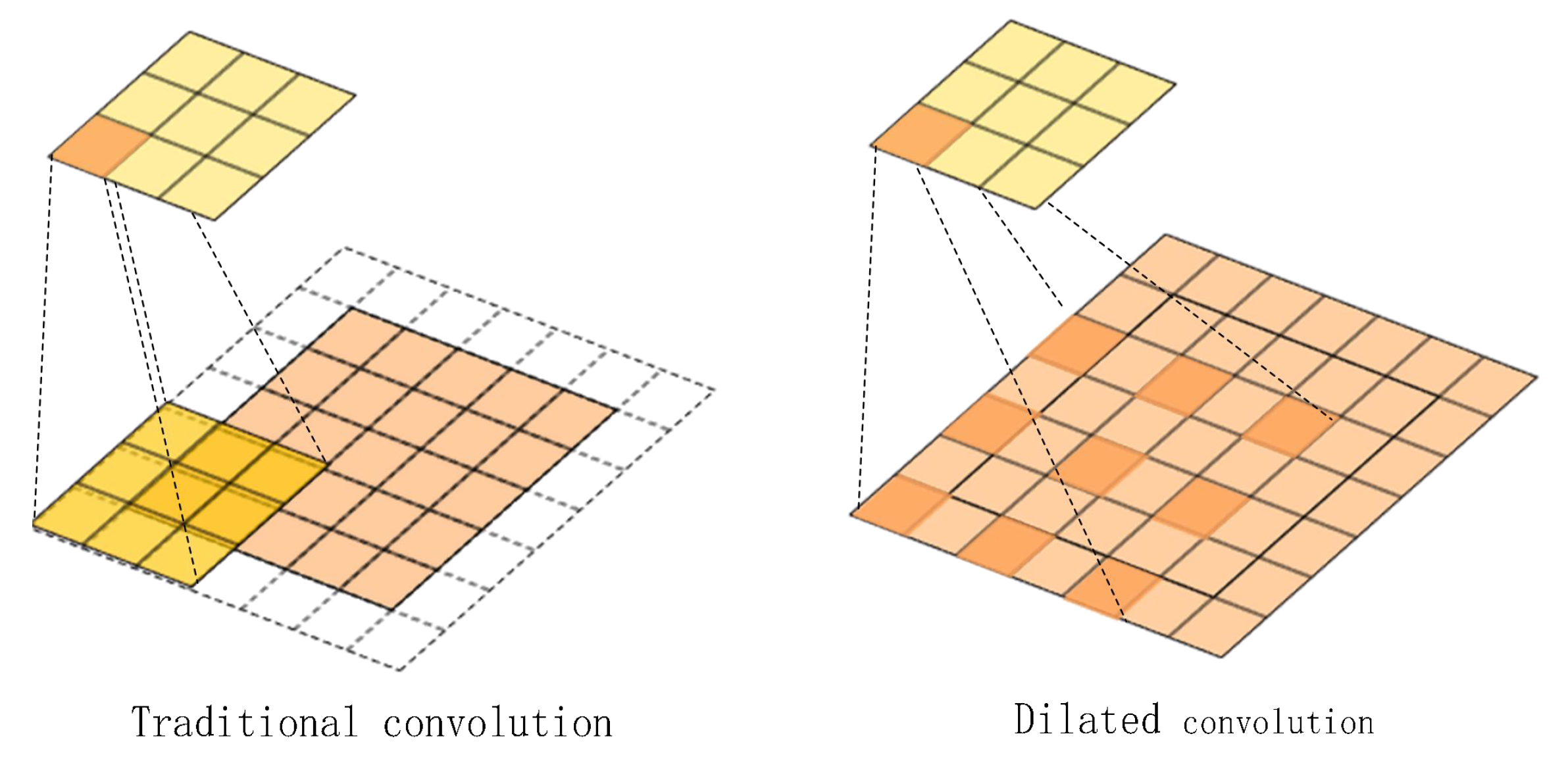
3.2. Introduction of SSD Network with Dilated Convolutional Structure
3.3. Introduction of Attention Mechanisms
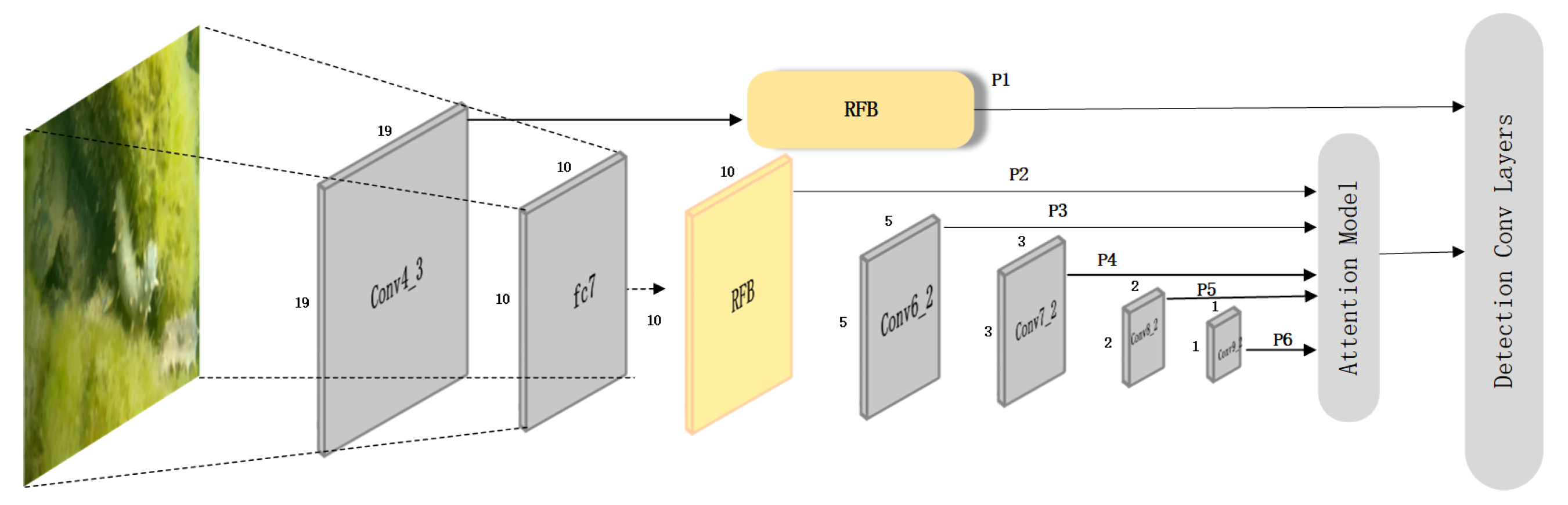
3.4. MobileNetv1 SSD Network with Attention Mechanisms
4. Experimental Results and Analysis
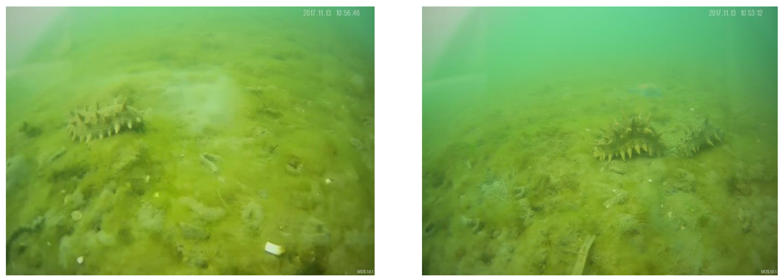
4.1. Experimental Data
4.2. Evaluation Index Setting
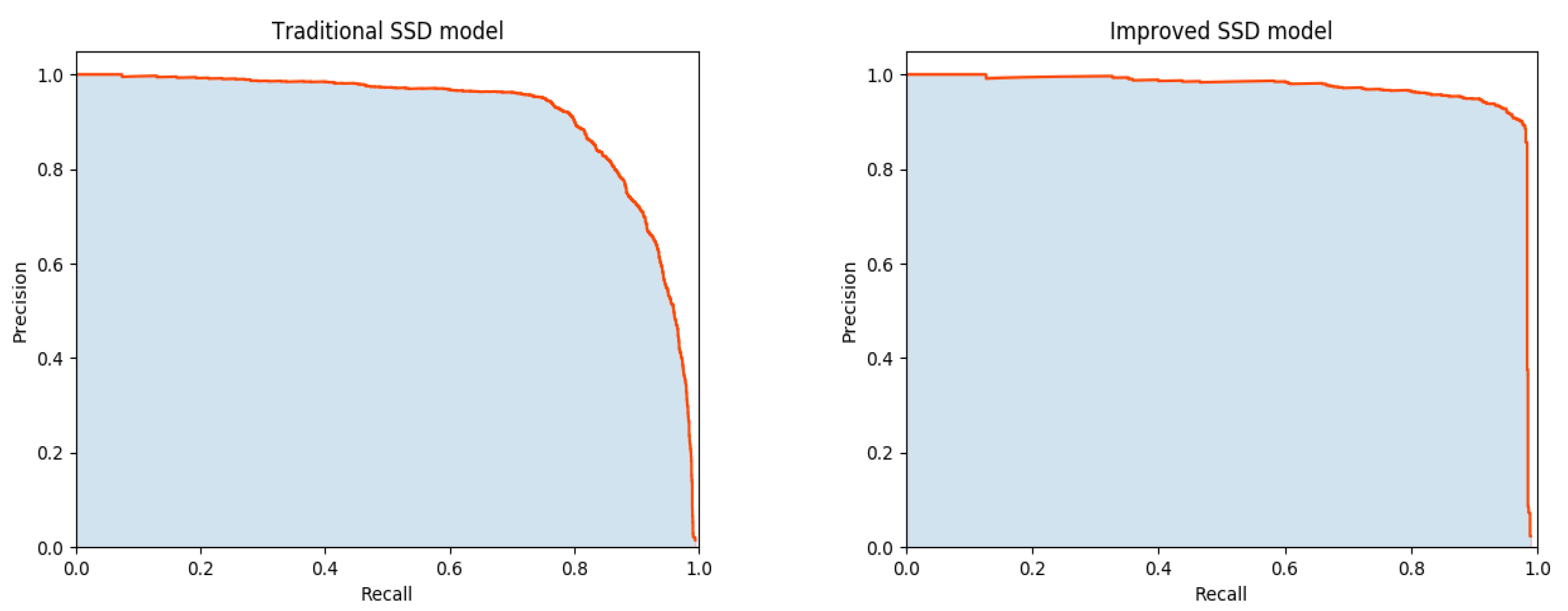
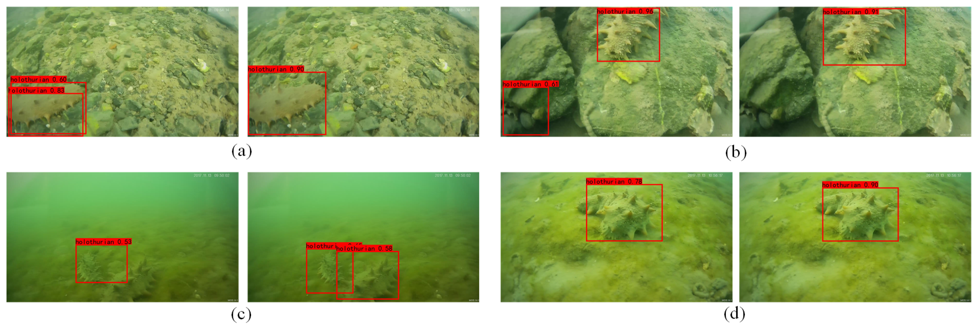
4.3. Improved SSD Model Validation
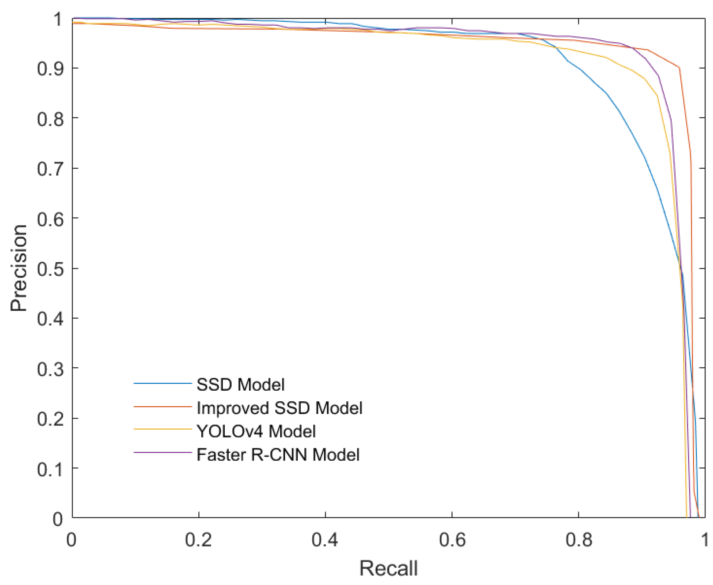
4.4. Comparison of Different Models
5. Conclusions
Author Contributions
Funding
Acknowledgments
Conflicts of Interest
Abbreviations
| SSD | Single Shot MultiBox Detector |
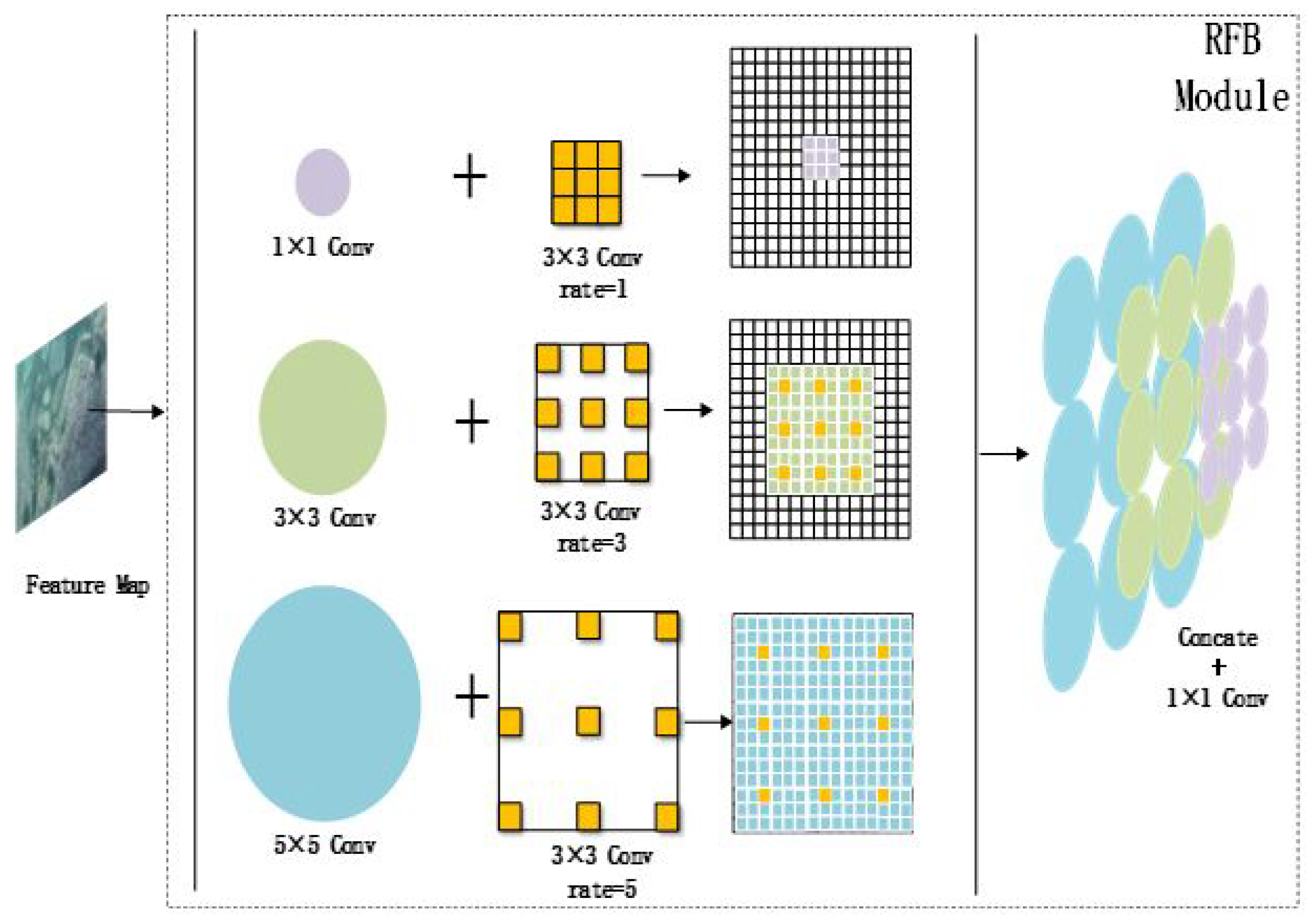
| RFB | Receptive Field Block |
References
- Ru, X.; Zhang, L.; Li, X.; Liu, S.; Yang, H. Development strategies for the sea cucumber industry in China. J. Ocean. Limnol. 2019, 37, 300–312. [Google Scholar] [CrossRef]
- Daniel Azari, B.G.; Daniel, R.S.; Walsalam, G.I. Sea cucumber aquaculture business potential in Middle East and South-East Asia-Pathways for ecological, social and economic sustainability. Surv. Fish. Sci. 2021, 7, 113–121. [Google Scholar] [CrossRef]
- Li, J.; Xu, C.; Jiang, L.; Xiao, Y.; Deng, L.; Han, Z. Detection and Analysis of Behavior Trajectory for Sea Cucumbers Based on Deep Learning. IEEE Access 2020, 8, 18832–18840. [Google Scholar] [CrossRef]
- Zhang, H.; Yu, F.; Sun, J.; Shen, X.; Li, K. Deep learning for sea cucumber detection using stochastic gradient descent algorithm. Eur. J. Remote Sens. 2020, 53, 53–62. [Google Scholar] [CrossRef] [Green Version]
- Wang, Q.; Li, S.; Qin, H.; Hao, A. Super-Resolution of Multi-Observed RGB-D Images Based on Nonlocal Regression and Total Variation. IEEE Trans. Image Process. 2016, 25, 1425–1440. [Google Scholar] [CrossRef] [PubMed]
- Guo, X.; Zhao, X.; Liu, Y. Underwater sea cucumber identification via deep residual networks. Inf. Process. Agric. 2019, 6, 307–315. [Google Scholar] [CrossRef]
- NgoGia, T.; Li, Y.; Jin, D.; Guo, J.; Li, J.; Tang, Q. Real-Time Sea Cucumber Detection Based on YOLOv4-Tiny and Transfer Learning Using Data Augmentation. In Advances in Swarm Intelligence; Tan, Y., Shi, Y., Eds.; Lecture Notes in Computer Science; Springer International Publishing: Cham, Switzerland, 2021; Volume 12690, pp. 119–128. [Google Scholar]
- Liu, W.; Anguelov, D.; Erhan, D.; Szegedy, C.; Reed, S.; Fu, C.-Y.; Berg, A.C. SSD: Single Shot MultiBox Detector. In Proceedings of the Computer Vision—ECCV 2016, Amsterdam, The Netherlands, 11–14 October 2016; pp. 21–37. [Google Scholar]
- Ning, C.; Zhou, H.; Song, Y.; Tang, J. Inception Single Shot MultiBox Detector for object detection. In Proceedings of the 2017 IEEE International Conference on Multimedia & Expo Workshops (ICMEW), Hong Kong, China, 10–14 July 2017; pp. 549–554. [Google Scholar]
- Huanjie, C.; Qiqi, W.; Guowei, Y.; Jialin, H.A.N.; Chengjuan, Y.I.N.; Jun, C.; Yizhong, W. SSD Object Detection Algorithm with Multi-Scale Convolution Feature Fusion. J. Front. Comput. Sci. Technol. 2019, 13, 1049. [Google Scholar]
- Shen, Z.; Liu, Z.; Li, J.; Jiang, Y.-G.; Chen, Y.; Xue, X. DSOD: Learning Deeply Supervised Object Detectors From Scratch. In Proceedings of the IEEE International Conference on Computer Vision, Venice, Italy, 22–29 October 2017; pp. 1919–1927. [Google Scholar]
- Kumar, A.; Zhang, Z.J.; Lyu, H. Object detection in real time based on improved single shot multi-box detector algorithm. J. Wirel. Commun. Netw. 2020, 2020, 1–18. [Google Scholar] [CrossRef]
- Arora, A.; Grover, A.; Chugh, R.; Reka, S.S. Real Time Multi Object Detection for Blind Using Single Shot Multibox Detector. Wirel. Pers. Commun. 2019, 107, 651–661. [Google Scholar] [CrossRef]
- Leng, J.; Liu, Y. An enhanced SSD with feature fusion and visual reasoning for object detection. Neural Comput. Appl. 2019, 31, 6549–6558. [Google Scholar] [CrossRef]
- Nguyen, A.Q.; Nguyen, H.T.; Tran, V.C.; Pham, H.X.; Pestana, J. A Visual Real-time Fire Detection using Single Shot MultiBox Detector for UAV-based Fire Surveillance. In Proceedings of the 2020 IEEE Eighth International Conference on Communications and Electronics (ICCE), Phu Quoc Island, Vietnam, 13–15 January 2021; pp. 338–343. [Google Scholar]
- Chen, H.Y.; Su, C.Y. An Enhanced Hybrid MobileNet. In Proceedings of the 2018 9th International Conference on Awareness Science and Technology (iCAST), Fukuoka, Japan, 19–21 September 2018; pp. 308–312. [Google Scholar]
- Sinha, D.; El-Sharkawy, M. Thin MobileNet: An Enhanced MobileNet Architecture. In Proceedings of the 2019 IEEE 10th Annual Ubiquitous Computing, Electronics & Mobile Communication Conference (UEMCON), New York, NY, USA, 10–12 October 2019; pp. 0280–0285. [Google Scholar]
- Hsiao, S.F.; Tsai, B.C. Efficient Computation of Depthwise Separable Convolution in MoblieNet Deep Neural Network Models. In Proceedings of the 2021 IEEE International Conference on Consumer Electronics-Taiwan (ICCE-TW), Penghu, Taiwan, 15–17 September 2021; pp. 1–2. [Google Scholar]
- Liu, S.; Huang, D.; Wang, Y. Receptive Field Block Net for Accurate and Fast Object Detection. In Proceedings of the European Conference on Computer Vision (ECCV), Munich, Germany, 8–14 September 2018; pp. 385–400. [Google Scholar]
- Yuan, Z.; Liu, Z.; Zhu, C.; Qi, J.; Zhao, D. Object Detection in Remote Sensing Images via Multi-Feature Pyramid Network with Receptive Field Block. Remote Sens. 2021, 13, 862. [Google Scholar] [CrossRef]
- Feng, H.; Guo, J.; Xu, H.; Ge, S.S. SharpGAN: Dynamic Scene Deblurring Method for Smart Ship Based on Receptive Field Block and Generative Adversarial Networks. Sensors 2021, 21, 3641. [Google Scholar] [CrossRef] [PubMed]
- XiaoFan, L.; HaiBo, P.; Yi, W.; JiangChuan, L.; HongXiang, X. Introduce GIoU into RFB net to optimize object detection bounding box. In Proceedings of the Proceedings of the 5th International Conference on Communication and Information Processing, Chongqing, China, 15–17 November 2019; Association for Computing Machinery: New York, NY, USA, 2019; pp. 108–113. [Google Scholar]
- Jin, F.; Liu, X.; Liu, Z.; Rui, J.; Guan, K. A Target Recognition Algorithm in Remote Sensing Images. In Proceedings of the 6th International Symposium of Space Optical Instruments and Applications, Delft, The Netherlands, 24–25 September 2019; pp. 133–142. [Google Scholar]
- Liu, S.; Huang, D.; Wang, Y. Adaptive NMS: Refining Pedestrian Detection in a Crowd. In Proceedings of the IEEE/CVF Conference on Computer Vision and Pattern Recognition (CVPR), Long Beach, CA, USA, 15–20 June 2019; pp. 6459–6468. [Google Scholar]
- Zhang, J.; Zhao, Z.; Su, F. Efficient-Receptive Field Block with Group Spatial Attention Mechanism for Object Detection. In Proceedings of the 2020 25th International Conference on Pattern Recognition (ICPR), Milan, Italy, 10–15 January 2021; pp. 3248–3255. [Google Scholar]
- Fukui, H.; Hirakawa, T.; Yamashita, T.; Fujiyoshi, H. Attention Branch Network: Learning of Attention Mechanism for Visual Explanation. In Proceedings of the IEEE/CVF Conference on Computer Vision and Pattern Recognition (CVPR), Long Beach, CA, USA, 15–20 June 2019; pp. 10705–10714. [Google Scholar]
- Li, Y.; Zeng, J.; Shan, S.; Chen, X. Occlusion Aware Facial Expression Recognition Using CNN With Attention Mechanism. IEEE Trans. Image Process. 2019, 28, 2439–2450. [Google Scholar] [CrossRef] [PubMed]
- Choi, E.; Bahadori, M.T.; Sun, J.; Kulas, J.; Schuetz, A.; Stewart, W. RETAIN: An Interpretable Predictive Model for Healthcare using Reverse Time Attention Mechanism. In Proceedings of the Annual Conference on Neural Information Processing Systems, Barcelona, Spain, 5–10 December 2016; Curran Associates, Inc.: Red Hook, NY, USA, 2016; Volume 29. [Google Scholar]
- Tao, C.; Gao, S.; Shang, M.; Wu, W.; Zhao, D.; Yan, R. Get The Point of My Utterance! Learning Towards Effective Responses with Multi-Head Attention Mechanism. In Proceedings of the Twenty-Seventh International Joint Conference on Artificial Intelligence, Stockholm, Sweden, 13–19 July 2018; p. 4424. [Google Scholar]
- Chen, Y.; Liu, L.; Phonevilay, V.; Gu, K.; Xia, R.; Xie, J.; Zhang, Q.; Yang, K. Image super-resolution reconstruction based on feature map attention mechanism. Appl. Intell. 2021, 51, 4367–4380. [Google Scholar] [CrossRef]
- Jiang, H.; Shi, T.; Bai, Z.; Huang, L. AHCNet: An Application of Attention Mechanism and Hybrid Connection for Liver Tumor Segmentation in CT Volumes. IEEE Access 2019, 7, 24898–24909. [Google Scholar] [CrossRef]
- Shang, T.; Dai, Q.; Zhu, S.; Yang, T.; Guo, Y. Perceptual Extreme Super-Resolution Network With Receptive Field Block. In Proceedings of the IEEE/CVF Conference on Computer Vision and Pattern Recognition (CVPR) Workshops, Virtual, 14–19 June 2020; pp. 440–441. [Google Scholar]
- Li, X.; Yang, Z.; Wu, H. Face Detection Based on Receptive Field Enhanced Multi-Task Cascaded Convolutional Neural Networks. IEEE Access 2020, 8, 174922–174930. [Google Scholar] [CrossRef]


| Detection method | Frames per Second | No. of Iterations | |
|---|---|---|---|
| Traditional SSD algorithms | 0.914 | 5.916 | 100 |
| Improved algorithm | 0.965 | 24.430 | 100 |
Publisher’s Note: MDPI stays neutral with regard to jurisdictional claims in published maps and institutional affiliations. |
© 2022 by the authors. Licensee MDPI, Basel, Switzerland. This article is an open access article distributed under the terms and conditions of the Creative Commons Attribution (CC BY) license (https://creativecommons.org/licenses/by/4.0/).
Share and Cite
Zhang, L.; Xing, B.; Wang, W.; Xu, J. Sea Cucumber Detection Algorithm Based on Deep Learning. Sensors 2022, 22, 5717. https://doi.org/10.3390/s22155717
Zhang L, Xing B, Wang W, Xu J. Sea Cucumber Detection Algorithm Based on Deep Learning. Sensors. 2022; 22(15):5717. https://doi.org/10.3390/s22155717
Chicago/Turabian StyleZhang, Lan, Bowen Xing, Wugui Wang, and Jingxiang Xu. 2022. "Sea Cucumber Detection Algorithm Based on Deep Learning" Sensors 22, no. 15: 5717. https://doi.org/10.3390/s22155717
APA StyleZhang, L., Xing, B., Wang, W., & Xu, J. (2022). Sea Cucumber Detection Algorithm Based on Deep Learning. Sensors, 22(15), 5717. https://doi.org/10.3390/s22155717