
Looseness Identification of Track Fasteners Based on Ultra-Weak FBG Sensing Technology and Convolutional Autoencoder Network


Abstract
:1. Introduction
2. Field Experiment for Generating the Fastener Looseness Dataset
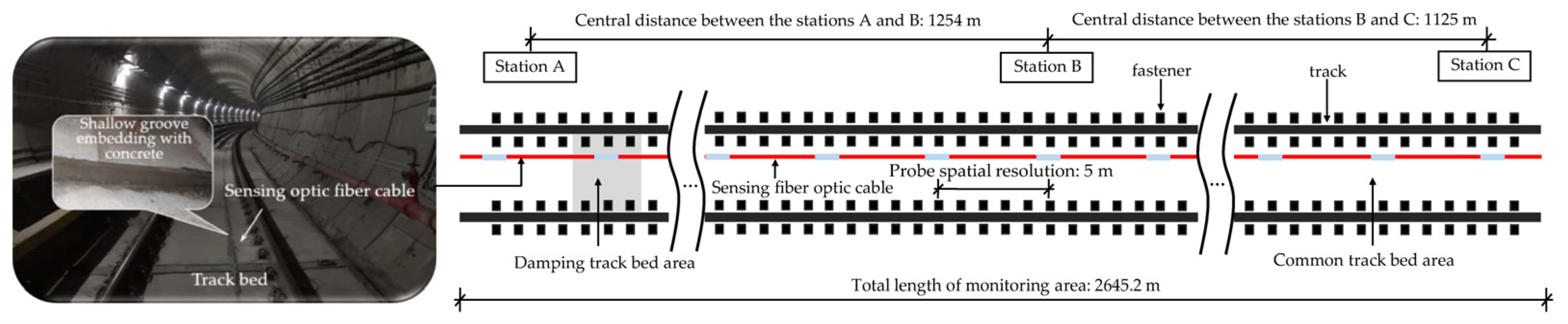
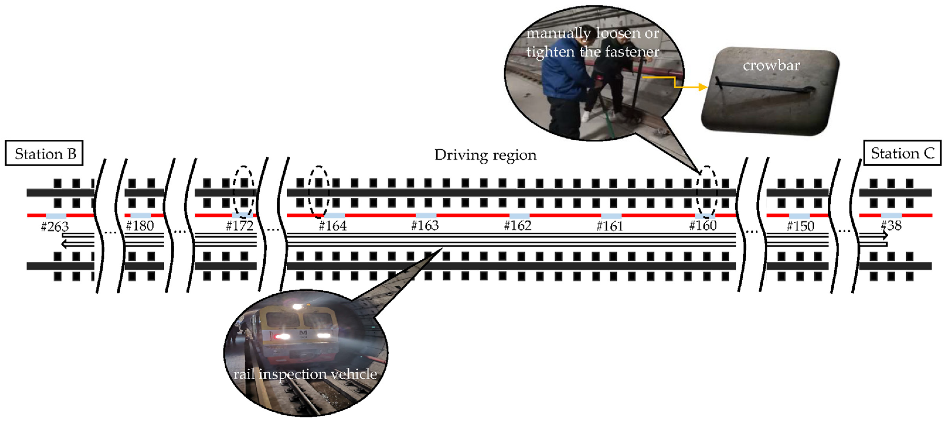
2.1. Background of Vibration Signal Acquisition
2.2. Design and Arrangement of Experimental Cases
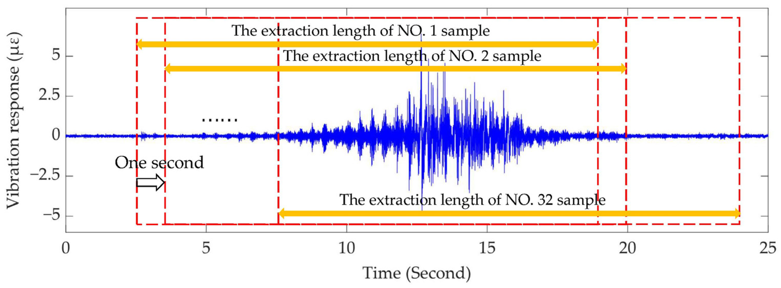
2.3. Dataset and Its Division and Usage
3. Methodology for Identification of Fastener Looseness
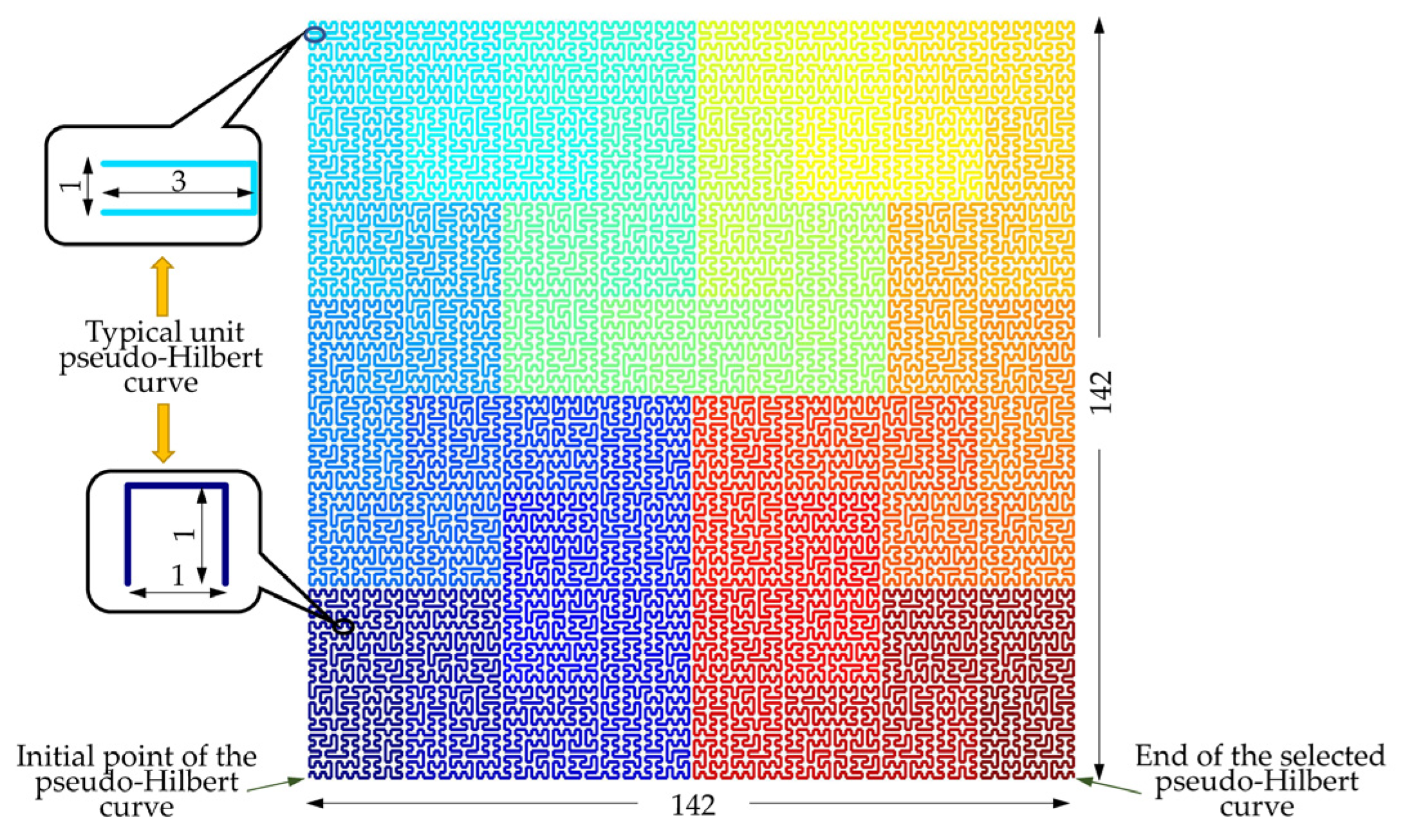
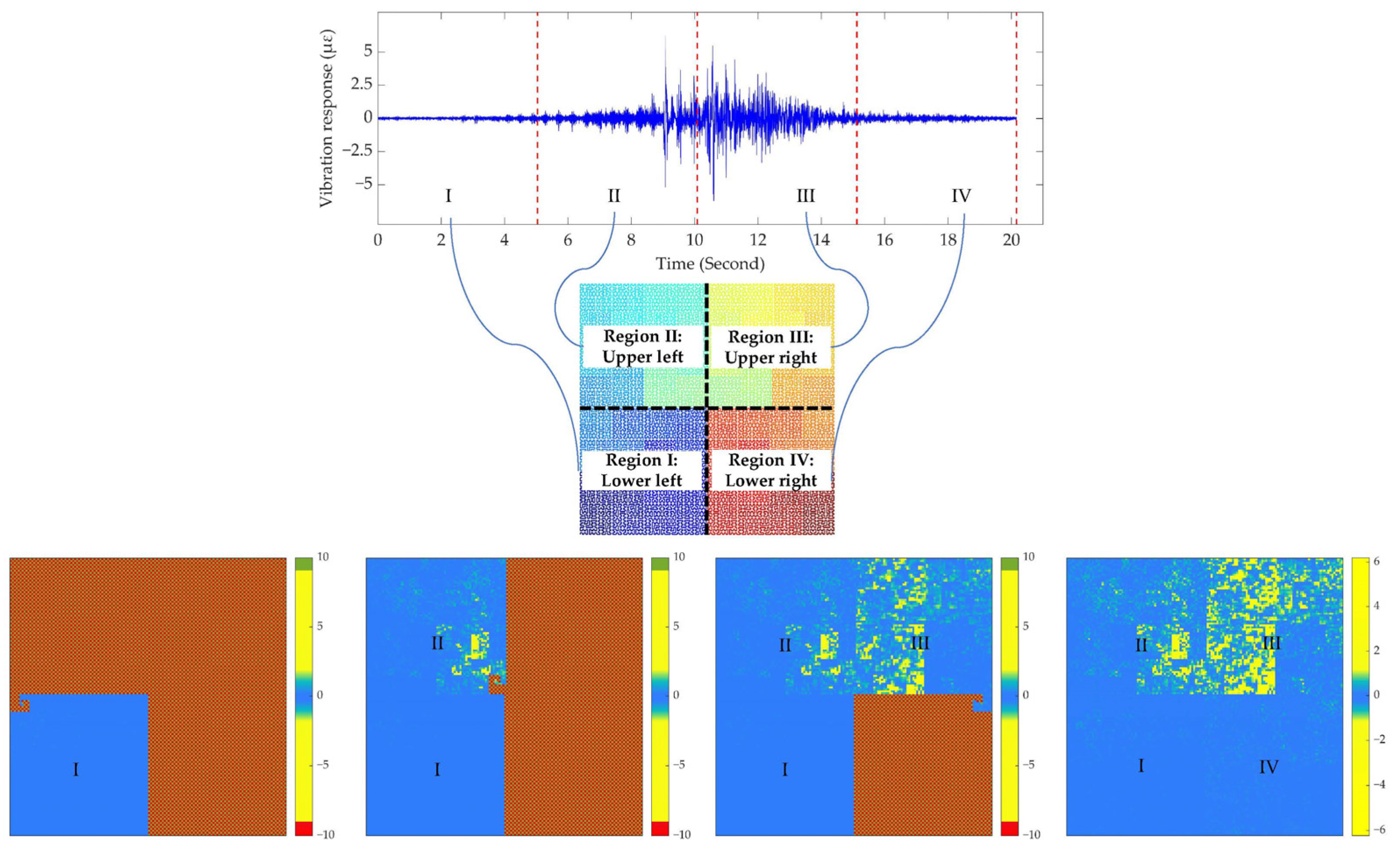
3.1. Pseudo-Hilbert Scan Operation
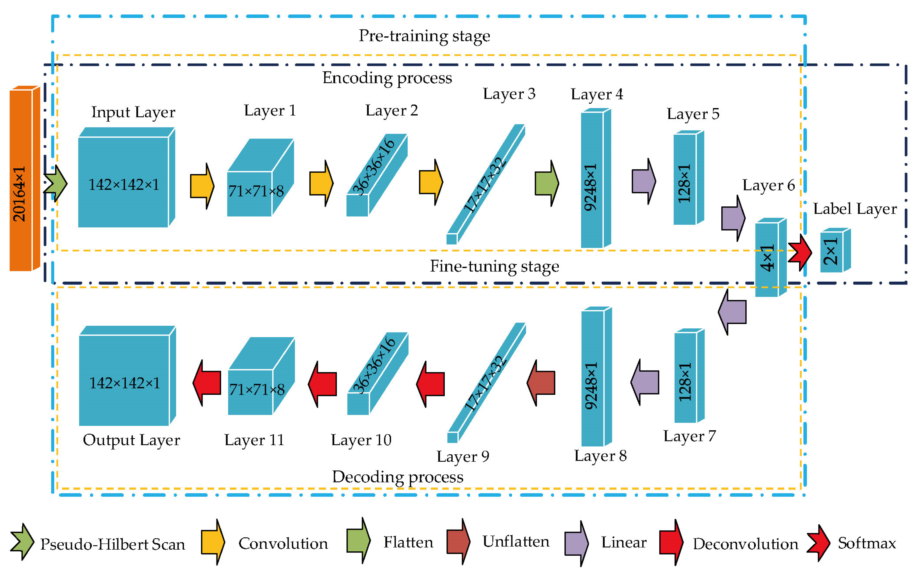
3.2. Establishment of CAE Network
4. Results, Analysis, and Discussion
5. Conclusions
Author Contributions
Funding
Institutional Review Board Statement
Informed Consent Statement
Data Availability Statement
Acknowledgments
Conflicts of Interest
References
- Nordmark, A. Fire and life safety for underground facilities: Present status of fire and life safety principles related to underground facilities. Tunn. Undergr. Space Technol. 1998, 13, 217–269. [Google Scholar] [CrossRef]
- Liu, Z.; Kim, A.K. Review of recent developments in fire detection technologies. J. Fire Prot. Eng. 2003, 13, 129–151. [Google Scholar] [CrossRef] [Green Version]
- Jiang, D.; Zhou, C.; Yang, M.; Li, S.; Wang, H. Research on optic fiber sensing engineering technology. In Proceedings of the 22nd International Conference on Optical Fiber Sensors, Beijing, China, 15–19 October 2012. [Google Scholar]
- Pamukcu, S.; Cheng, L.; Pervizpour, M. Chapter 1—Introduction and overview of underground sensing for sustainable response. In Underground Sensing. Monitoring and Hazard Detection for Environment and Infrastructure, 1st ed.; Pamukcu, S., Cheng, L., Eds.; Academic Press: Cambridge, MA, USA, 2018; pp. 1–42. [Google Scholar]
- Soga, K.; Kechavarzi, C.; Pelecanos, L.; Battista, N.; Williamson, M.; Gue, C.Y.; Murro, V.D.; Elshafie, M.; Monzón-Hernández, D., Sr.; Bustos, E.; et al. Chapter 6—Fiber-optic underground sensor networks. In Underground Sensing. Monitoring and Hazard Detection for Environment and Infrastructure, 1st ed.; Pamukcu, S., Cheng, L., Eds.; Academic Press: Cambridge, MA, USA, 2018; pp. 287–356. [Google Scholar]
- Chen, X.; Li, X.; Zhu, H. Condition evaluation of urban metro shield tunnels in Shanghai through multiple indicators multiple causes model combined with multiple regression method. Undergr. Space Technol. 2019, 85, 170–181. [Google Scholar] [CrossRef]
- Das, S.; Saha, P. A review of some advanced sensors used for health diagnosis of civil engineering structures. Meas. J. Int. Meas. Confed. 2018, 129, 68–90. [Google Scholar] [CrossRef]
- Huang, J.; Zhang, W.; Huang, W.; Huang, W.; Wang, L.; Luo, Y. High-resolution fiber optic seismic sensor array for intrusion detection of subway tunnel. In Proceedings of the 2018 Asia Communications and Photonics Conference (ACP), Hangzhou, China, 26–29 October 2018. [Google Scholar]
- Yu, Z.; Liu, F.; Yuan, Y.; Li, S.; Li, Z. Signal processing for time domain wavelengths of ultra-weak FBGs array in perimeter security monitoring based on spark streaming. Sensors 2018, 18, 2937. [Google Scholar] [CrossRef] [Green Version]
- Hoentsch, J.; Scholz, S. Reliable detection of security camera misalignment in urban rail environments. In Proceedings of the 2018 Joint Rail Conference, JRC 2018, Pittsburgh, PA, USA, 19–20 April 2018. [Google Scholar]
- Gan, W.; Li, S.; Li, Z.; Sun, L. Identification of ground intrusion in underground structures based on distributed structural vibration detected by ultra-weak FBG sensing technology. Sensors 2019, 19, 2160. [Google Scholar] [CrossRef] [Green Version]
- Nan, Q.; Li, S.; Yao, Y.; Li, Z.; Wang, H.; Wang, L.; Sun, L. A novel monitoring approach for train tracking and incursion detection in underground structures based on ultra-weak FBG sensing array. Sensors 2019, 19, 2666. [Google Scholar] [CrossRef] [Green Version]
- Remennikov, A.M.; Kaewunruen, S. A review of loading conditions for railway track structures due to train and track vertical interaction. J. Struct. Control Health Monit. 2008, 15, 207–234. [Google Scholar] [CrossRef]
- Jun, X.; Qingyuan, Z. A study on mechanical mechanism of train derailment and preventive measures for derailment. Veh. Syst. Dyn. 2005, 43, 121–147. [Google Scholar] [CrossRef]
- Kaewunruen, S.; Osman, M.H.; Hao Cheng Eric, W. Risk-based maintenance planning for rail fastening systems. ASCE-ASME J. Risk Uncertain. Eng. Syst. Part A Civ. Eng. 2019, 5, 04019007. [Google Scholar] [CrossRef] [Green Version]
- Ikshwaku, S.; Srinivasan, A.; Varghese, A.; Gubbi, J. Railway corridor monitoring using deep drone vision. In Computational Intelligence: Theories, Applications and Future Directions—Volume II. Advances in Intelligent Systems and Computing, 1st ed.; Verma, N., Ghosh, A.K., Eds.; Springer: Singapore, 2018; pp. 361–372. [Google Scholar]
- Wei, X.; Yang, Z.; Liu, Y.; Wei, D.; Jia, L.; Li, Y. Railway track fastener defect detection based on image processing and deep learning techniques: A comparative study. Eng. Appl. Artif. Intell. 2019, 80, 66–81. [Google Scholar] [CrossRef]
- Li, S.; Zuo, X.; Li, Z.; Wang, H.; Sun, L. Combining SDAE network with improved DTW algorithm for similarity measure of ultra-weak FBG vibration responses in underground structures. Sensors 2020, 20, 2179. [Google Scholar] [CrossRef] [Green Version]
- Luo, Z.; Wen, H.; Guo, H.; Yang, M. A time-and wavelength-division multiplexing sensor network with ultra-weak fiber Bragg gratings. Opt. Express 2013, 21, 22799–22807. [Google Scholar] [CrossRef] [Green Version]
- Wang, S.; Liu, D.; Yang, Z.; Feng, C.; Yao, R. A convolutional neural network image classification based on extreme learning machine. IAENG Int. J. Comput. Sci. 2021, 48, 1–5. [Google Scholar]
- Ye, C.; Yin, Z.; Zhao, M.; Tian, Y.; Sun, Z. Identification of mental fatigue levels in a language understanding task based on multi-domain EEG features and an ensemble convolutional neural network. Biomed. Signal Process. Control 2022, 72, 103360. [Google Scholar] [CrossRef]
- Fan, Q. The application of minority music style recognition based on deep convolution loop neural network. Wireless Commun. Mobile Comput. 2022, 2022, 4556135. [Google Scholar] [CrossRef]
- Tang, Z.; Chen, Z.; Bao, Y.; Li, H. Convolutional neural network-based data anomaly detection method using multiple information for structural health monitoring. J. Struct. Control Health Monit. 2019, 26, 2296. [Google Scholar] [CrossRef] [Green Version]
- Li, S.; Sun, L. Detectability of bridge-structural damage based on fiber-optic sensing through deep-convolutional neural networks. J. Bridge Eng. 2020, 25, 04020012. [Google Scholar] [CrossRef]
- Abdeljaber, O.; Avci, O.; Kiranyaz, M.S.; Boashash, B.; Sodano, H.; Inman, D.J. 1-D CNNs for structural damage detection: Verification on a structural health monitoring benchmark data. Neurocomputing 2018, 275, 1308–1317. [Google Scholar] [CrossRef]
- Dhar, P.; Garg, V.K.; Rahman, M.A. Enhanced feature extraction-based CNN approach for epileptic seizure detection from EEG signals. J. Healthc. Eng. 2022, 2022, 3491828. [Google Scholar] [CrossRef]
- Hasan, M.J.; Islam, M.M.M.; Kim, J. Acoustic spectral imaging and transfer learning for reliable bearing fault diagnosis under variable speed conditions. Meas. J. Int Meas. Confed. 2019, 138, 620–631. [Google Scholar] [CrossRef]
- Li, Y.; Cheng, G.; Pang, Y.; Kuai, M. Planetary gear fault diagnosis via feature image extraction based on multi central frequencies and vibration signal frequency spectrum. Sensors 2018, 18, 1735. [Google Scholar] [CrossRef] [Green Version]
- Hoang, D.; Kang, H. Rolling element bearing fault diagnosis using convolutional neural network and vibration image. Cogn. Syst. Res. 2019, 53, 42–50. [Google Scholar] [CrossRef]
- Yu, H.; Tao, J.; Qin, C.; Liu, M.; Xiao, D.; Sun, H.; Liu, C. A novel constrained dense convolutional autoencoder and DNN-based semi-supervised method for shield machine tunnel geological formation recognition. Mech. Syst. Signal Process. 2022, 165, 108353. [Google Scholar] [CrossRef]
- Zhang, H.; Tang, W.; Zhang, L.; Li, P.; Gu, D. Defect detection of yarn-dyed shirts based on denoising convolutional self-encoder. In Proceedings of the 8th IEEE Data Driven Control and Learning Systems Conference, Dali, China, 24–27 May 2019. [Google Scholar]
- Zhang, E.; Seiler, S.; Chen, M.; Lu, W.; Gu, X. Boundary-aware semi-supervised deep learning for breast ultrasound computer-aided diagnosis. In Proceedings of the 41st Annual International Conference of the IEEE Engineering in Medicine and Biology Society, Berlin, Germany, 23–27 July 2019. [Google Scholar]
- Tsinganos, P.; Cornelis, B.; Cornelis, J.; Jansen, B.; Skodras, A. Hilbert sEMG data scanning for hand gesture recognition based on deep learning. Neural Comput. Appl. 2021, 33, 2645–2666. [Google Scholar] [CrossRef]
- Kamata, S.; Bandoh, Y. Address generator of a pseudo-Hilbert scan in a rectangle region. In Proceedings of the 1997 International Conference on Image Processing, Santa Barbara, CA, USA, 26–29 October 1997. [Google Scholar]
- Biswas, S. Hubert scan image compression. In Proceedings of the 15th International Conference on Pattern Recognition, Barcelona, Spain, 3–7 September 2000. [Google Scholar]
- Lu, W.; Yan, X. Industrial process data visualization based on a deep enhanced t-distributed stochastic neighbor embedding neural network. Assem. Autom. 2022, 42, 268–277. [Google Scholar] [CrossRef]
- Tong, Y.; Li, Z.; Wang, J.; Wang, H.; Yu, H. High-speed Mach-Zehnder-OTDR distributed optical fiber vibration sensor using medium-coherence laser. Photonic Sens. 2018, 8, 203–212. [Google Scholar] [CrossRef] [Green Version]
- Sitaula, C.; Hossain, M.B. Attention-based VGG-16 model for COVID-19 chest X-ray image classification. Appl. Intell. 2021, 51, 2850–2863. [Google Scholar] [CrossRef] [PubMed]
- Patro, S.G.K.; Sahu, K.K. Normalization: A preprocessing Stage. Available online: https://arxiv.org/abs/1503.06462 (accessed on 22 July 2022).
- Moon, B.; Jagadish, H.V.; Faloutsos, C.; Saltz, J.H. Analysis of the clustering properties of the Hilbert space-filling curve. IEEE Trans. Knowl. Data Eng. 2001, 13, 124–141. [Google Scholar] [CrossRef] [Green Version]
- Zhang, J.; Kamata, S. A generalized 3-D Hilbert scan using look-up tables. J. Visual Commun. Image Represent. 2012, 23, 418–425. [Google Scholar] [CrossRef]
- Zhang, J.; Kamata, S.; Ueshige, Y. A pseudo-Hilbert scan algorithm for arbitrarily-sized rectangle region. In Proceedings of the International Workshop on Intelligent Computing in Pattern Analysis/Synthesis, Xi’an, China, 26–27 August 2006. [Google Scholar]
- Han, Z.; Li, J.; Zhang, B.; Hossain, M.M.; Xu, C. Prediction of combustion state through a semi-supervised learning model and flame imaging. Fuel 2021, 289, 119745. [Google Scholar] [CrossRef]
- Nair, V.; Hinton, G.E. Rectified linear units improve restricted Boltzmann machines. In Proceedings of the 27th International Conference on Machine Learning, Haifa, Israel, 21–25 June 2010. [Google Scholar]
- Lameski, P.; Zdravevski, E.; Mingov, R.; Kulakov, A. SVM parameter tuning with grid search and its impact on reduction of model over-fitting. In Rough Sets, Fuzzy Sets, Data Mining, and Granular Computing; Lecture Notes in Computer Science; Springer: Cham, Switzerland, 2015; Volume 9437, pp. 464–474. [Google Scholar]
- Ruder, S. An Overview of Gradient Descent Optimization Algorithms. Available online: https://arxiv.org/abs/1609.04747v2 (accessed on 22 July 2022).
- Kuo, K.M.; Talley, P.C.; Chang, C.S. The accuracy of machine learning approaches using non-image data for the prediction of COVID-19: A meta-analysis. Int. J. Med. Inf. 2022, 164, 104791. [Google Scholar] [CrossRef]
- Wang, R.; Li, J. Bayes test of precision, recall, and F1 measure for comparison of two natural language processing models. In Proceedings of the 57th Annual Meeting of the Association for Computational Linguistics, Florence, Italy, 28 July–2 August 2020. [Google Scholar]
- Atangana Njock, P.G.; Shen, S.; Zhou, A.; Lyu, H. Evaluation of soil liquefaction using AI technology incorporating a coupled ENN/t-SNE model. Soil Dyn. Earthqu. Eng. 2020, 130, 105988. [Google Scholar] [CrossRef]
- Bai, Y.; Feng, Y.; Wang, Y.; Dai, T.; Xia, S.; Jiang, Y. Hilbert-based Generative Defense for Adversarial Examples. In Proceedings of the 2019 IEEE/CVF International Conference on Computer Vision (ICCV), Seoul, Korea, 27 October–2 November 2019. [Google Scholar]
- Kamata, S.; Eason, R.O.; Bandou, Y. A new algorithm for N-dimensional Hilbert scanning. IEEE Trans. Image Process. 1999, 8, 964–973. [Google Scholar] [CrossRef]
- Zhang, Y.M.; Wang, H.; Mao, J.X.; Xu, Z.D.; Zhang, Y.F. Probabilistic framework with Bayesian optimization for predicting typhoon-induced dynamic responses of a long-span bridge. J. Struct. Eng. 2021, 147, 04020297. [Google Scholar] [CrossRef]
- Zhang, Y.M.; Wang, H.; Bai, Y.; Mao, J.X.; Xu, Y.C. Bayesian Dynamic Regression for Reconstructing Missing Data in Structural Health Monitoring. Struct. Health Monit. 2022. [Google Scholar] [CrossRef]
- Wan, H.P.; Ni, Y.Q. Bayesian multi-task learning methodology for reconstruction of structural health monitoring data. Struct. Health Monit. 2019, 18, 1282–1309. [Google Scholar] [CrossRef] [Green Version]


| State Number | Fastener State | Driving Direction | Travel Time |
|---|---|---|---|
| 1 | Before looseness | Station B→Station C | 0:58 a.m.–1:01 a.m. |
| Station C→Station B | 1:04 a.m.–1:07 a.m. | ||
| Station B→Station C | 1:10 a.m.–1:13 a.m. | ||
| Station C→Station B | 1:16 a.m.–1:19 a.m. | ||
| 2 | After looseness | Station B→Station C | 1:34 a.m.–1:37 a.m. |
| Station C→Station B | 1:40 a.m.–1:43 a.m. | ||
| Station B→Station C | 1:46 a.m.–1:49 a.m. | ||
| Station C→Station B | 1:52 a.m.–1:55 a.m. | ||
| 3 | Retighten | Station B→Station C | 2:06 a.m.–2:09 a.m. |
| Station C→Station B | 2:12 a.m.–2:15 a.m. | ||
| Station B→Station C | 2:18 a.m.–2:21 a.m. | ||
| Station C→Station B | 2:23 a.m.–2:26 a.m. |
| Label | Sample Source | Sample Size | |
|---|---|---|---|
| A: Fastener in the loose state | #160 | 4→32 | 96 |
| #164 | 4→32 | ||
| #172 | 4→32 | ||
| B: Fastener in the normal state | #160 | 4 + 4 = 8 | 396 |
| #164 | 4 + 4 = 8 | ||
| #172 | 4 + 4 = 8 | ||
| #150~#180 (except for #160, #164, and #172) | 31 × 12 = 372 | ||
| Dataset Division | Training Dataset Size | Test Dataset Size | |
|---|---|---|---|
| Pre-Training Stage | Fine-Tuning Stage | ||
| Label A | 67 | 67 | 29 |
| Label B | 277 | 67 | 119 |
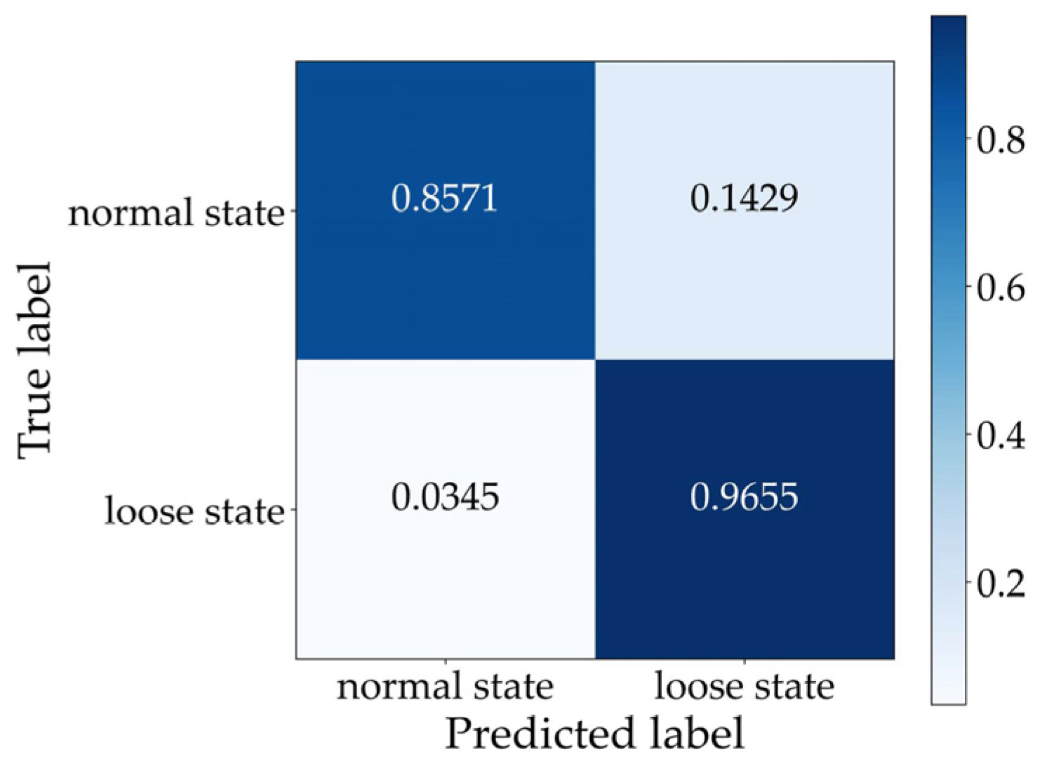
| Indicator | Accuracy | Precision | Recall | F1-Score |
|---|---|---|---|---|
| Result | 0.8784 | 0.9902 | 0.8571 | 0.9189 |
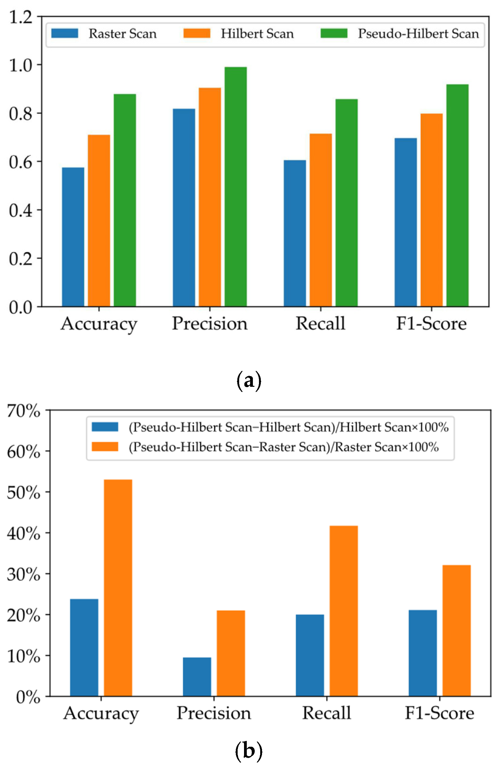
| Item | Accuracy | Precision | Recall | F1-Score | Identifiability |
|---|---|---|---|---|---|
| Pseudo-Hilbert scan | 0.8784 | 0.9902 | 0.8571 | 0.9189 | 87.39% |
| Raster scan | 0.5743 | 0.8181 | 0.605 | 0.6957 | chaos |
| Hilbert scan | 0.7095 | 0.9043 | 0.7143 | 0.7589 | 75.63% |
Publisher’s Note: MDPI stays neutral with regard to jurisdictional claims in published maps and institutional affiliations. |
© 2022 by the authors. Licensee MDPI, Basel, Switzerland. This article is an open access article distributed under the terms and conditions of the Creative Commons Attribution (CC BY) license (https://creativecommons.org/licenses/by/4.0/).
Share and Cite
Li, S.; Jin, L.; Jiang, J.; Wang, H.; Nan, Q.; Sun, L. Looseness Identification of Track Fasteners Based on Ultra-Weak FBG Sensing Technology and Convolutional Autoencoder Network. Sensors 2022, 22, 5653. https://doi.org/10.3390/s22155653
Li S, Jin L, Jiang J, Wang H, Nan Q, Sun L. Looseness Identification of Track Fasteners Based on Ultra-Weak FBG Sensing Technology and Convolutional Autoencoder Network. Sensors. 2022; 22(15):5653. https://doi.org/10.3390/s22155653
Chicago/Turabian StyleLi, Sheng, Liang Jin, Jinpeng Jiang, Honghai Wang, Qiuming Nan, and Lizhi Sun. 2022. "Looseness Identification of Track Fasteners Based on Ultra-Weak FBG Sensing Technology and Convolutional Autoencoder Network" Sensors 22, no. 15: 5653. https://doi.org/10.3390/s22155653
APA StyleLi, S., Jin, L., Jiang, J., Wang, H., Nan, Q., & Sun, L. (2022). Looseness Identification of Track Fasteners Based on Ultra-Weak FBG Sensing Technology and Convolutional Autoencoder Network. Sensors, 22(15), 5653. https://doi.org/10.3390/s22155653