
Unified DeepLabV3+ for Semi-Dark Image Semantic Segmentation

 , , ,
, , ,
Abstract
:1. Introduction
- The loss of spatial relationships by using per-pixel primitives, resulting in poorly detected object classes over boundary pixels.
- The limited representational power due to the use of identity shortcuts and the occurrence of an internal covariant shift during the training of DNNs.
- The constrained multiscale feature extraction caused by biased centric exploitations.
- 1.
- Proposal of a novel version of DeepLabV3+ for semi-dark imagery—Unified DeepLabV3+
- 2.
- Proposal of a novel evaluation metric—
2. Related Work
2.1. Feature-Encoder-Based Methods
2.2. Increased Resolution of Feature-Encoder-Based Methods
2.3. Critical Analysis of DeepLab Versions
- DeepLabV1
- 2.
- DeepLabV2
- 3.
- DeepLabV3
- 4.
- DeepLabV3+
2.4. Conclusive Deductions
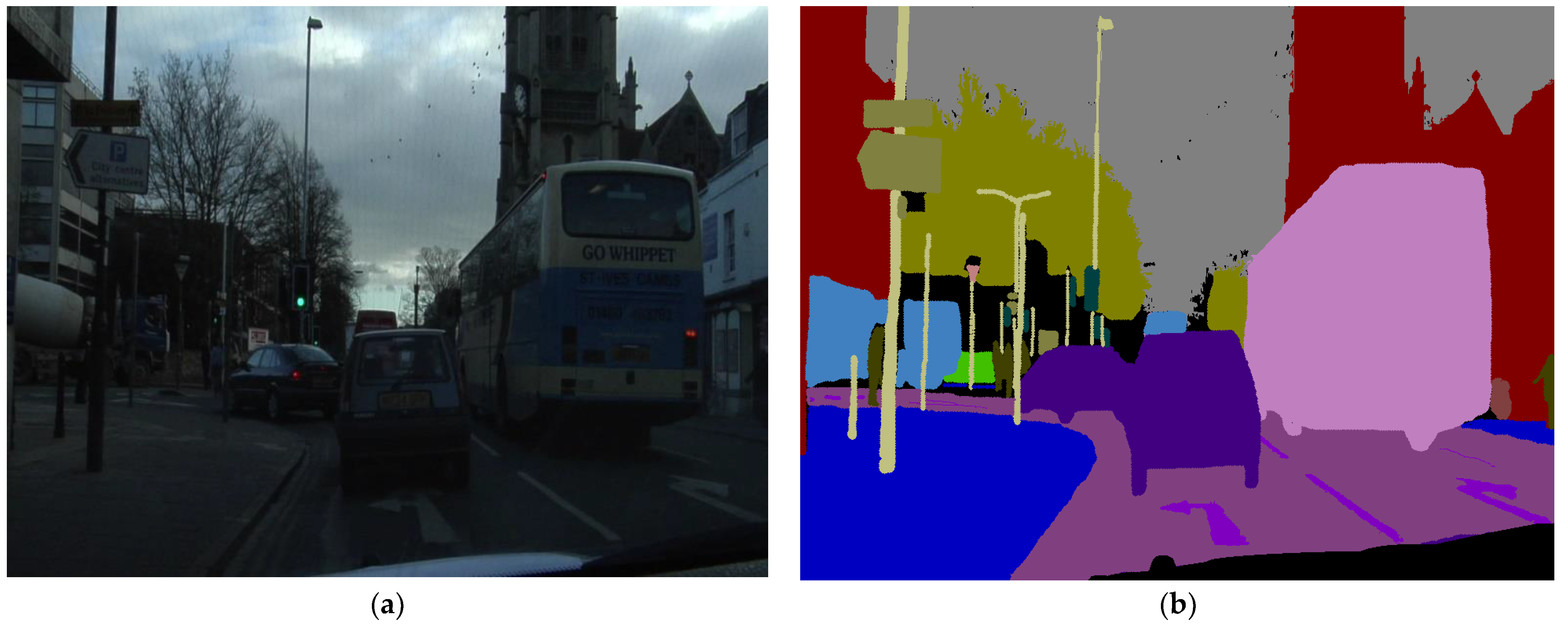
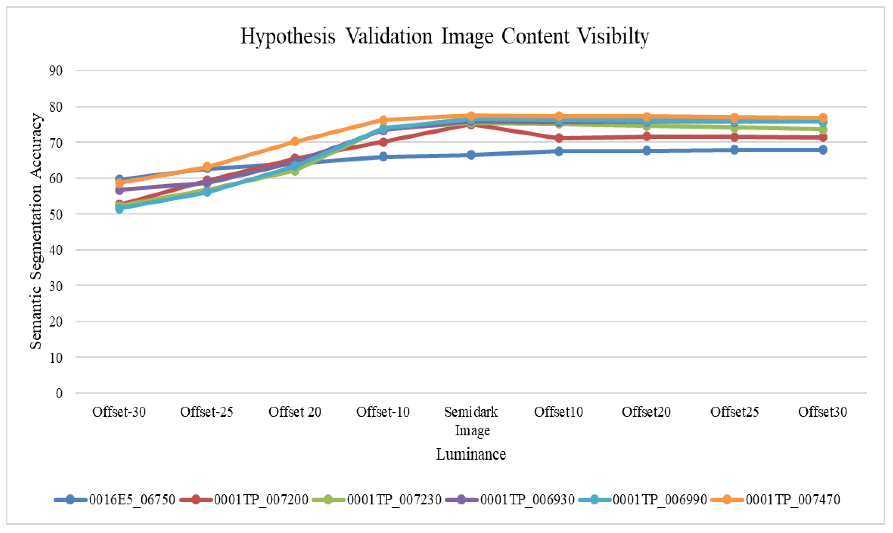
2.5. Preliminary Hypothesis Validation
3. Materials and Methods
3.1. Overview of Proposed Architecture
Rationale for Proposing an Ensemble Approach
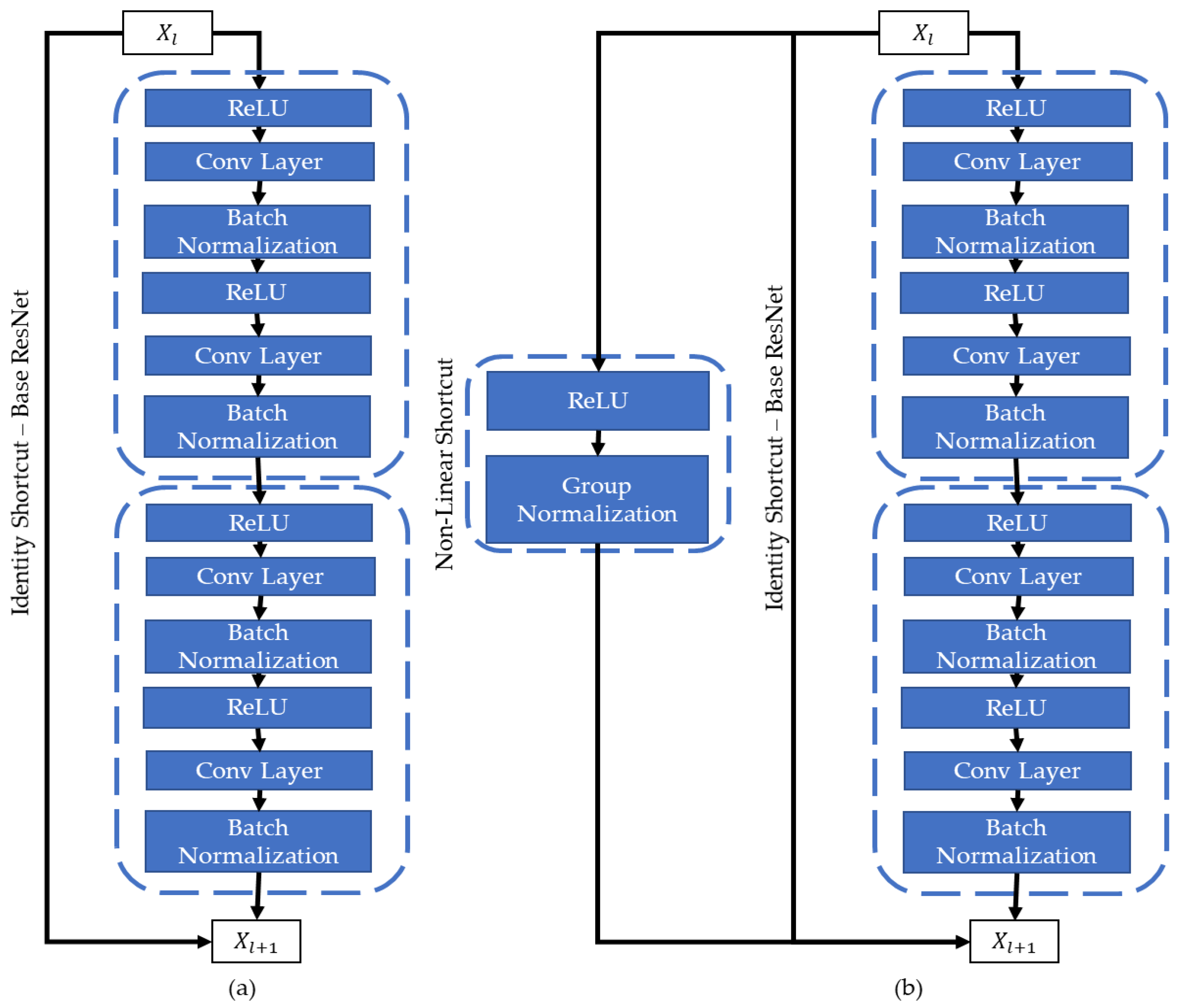
3.2. Encoder Enhancement—Non-Linear Shortcuts
3.3. MobileNetV2 Encoder
3.4. Decoder Enhancement—Customized Pyramid Module
3.5. Statistical Class-Wise Fusion
| Algorithm 1: Proposed Parallel DCNN for Semi-Dark Images |
| Input: Initial DCNN parameters RGSNet-DeepLab (Net1), MobNet-DeepLab (Net2), Custom-DeepLab (Net3), customization parameters (including expansion rate, dilation rate, and group normalization number), segmented image with pixels, pixel label set to (1 → n, no of classes). |
| Parallel DCNN Processing Steps: 1: For each image pixel m, all three DCNN variants perform given . 2: Every pixel (m → M, where M is the no. of image pixels) of image receives a semantic label from Net1, Net2, and Net3. |
| Statistical Class-wise Fusion Step: 3: Class-wise mapping is achieved using |
| where is a class-wise label generated from Net1, is a class-wise label generated from Net2, and is a class-wise label generated from Net3. |
| Output: Semantic segmentation pixel mask representing object classes. |
| Algorithm 2: Parallel DCNN Class-Wise Fusion | |
| 1: | Provided class-wise results of RGSNet (), CustomDecoder-DeepLabV3+ (, and MobileNet-DeepLabV3+ ( |
| 2: | Compare (), (, and ( |
| 3: | For each object class |
| 4: | If () > () && () > () |
| 5: | Store in stack |
| 6: | Else If () > () && () > () |
| 7: | Store in stack |
| 8: | Else If () > () && () > () |
| 9: | Store in stack |
| 10: | Create a final semantic segmentation vector by fetching the stack values |
4. Experiments
4.1. Dataset and Evaluation Metrics
4.1.1. Proposal of Novel Evaluation Criteria
Significance of Proposed Evaluation Criteria
Experimental Protocol for Weight Identification of
| Algorithm 3: Incremental IoU | |
| 1: | Initialize weights (weight for OA), (weight for IoU), (weight for MeanBFScore), and Overall_Weight W |
| 2: | Set = 0.001 |
| 3: | Repeat until W2 == 1 |
| 4: | Set |
| 5: | Set |
| 6: | |
| 7: | |
| 8: | If W > 1 |
| 9: | Break |
| Algorithm 4: Incremental MeanBFScore | |
| 1: | Initialize weights (weight for OA), (weight for IoU), (weight for MeanBFScore), and Overall_Weight W |
| 2: | Set = 0.001 |
| 3: | Repeat until W3 == 1 |
| 4: | Set |
| 5: | Set |
| 6: | |
| 7: | |
| 8: | If W > 1 |
| 9: | Break |
| Algorithm 5: Incremental OA | |
| 1: | Initialize weights (weight for OA), (weight for IoU), (weight for MeanBFScore), and Overall_Weight W |
| 2: | Set = 0.001 |
| 3: | Repeat until W1 == 1 |
| 4: | Set |
| 5: | Set |
| 6: | |
| 7: | |
| 8: | If W > 1 |
| 9: | Break |
| Algorithm 6: Randomized Weights | |
| 1: | Initialize weights (weight for OA), (weight for IoU), (weight for MeanBFScore), Overall_Weight W and counter C |
| 2: | Set C = 1 |
| 3: | Repeat until C <= 1000 |
| 4: | Set |
| 5: | Set |
| 6: | Set = ) |
| 7: | |
| 8: | |
| 9: | If W > 1 |
| 10: | Break |
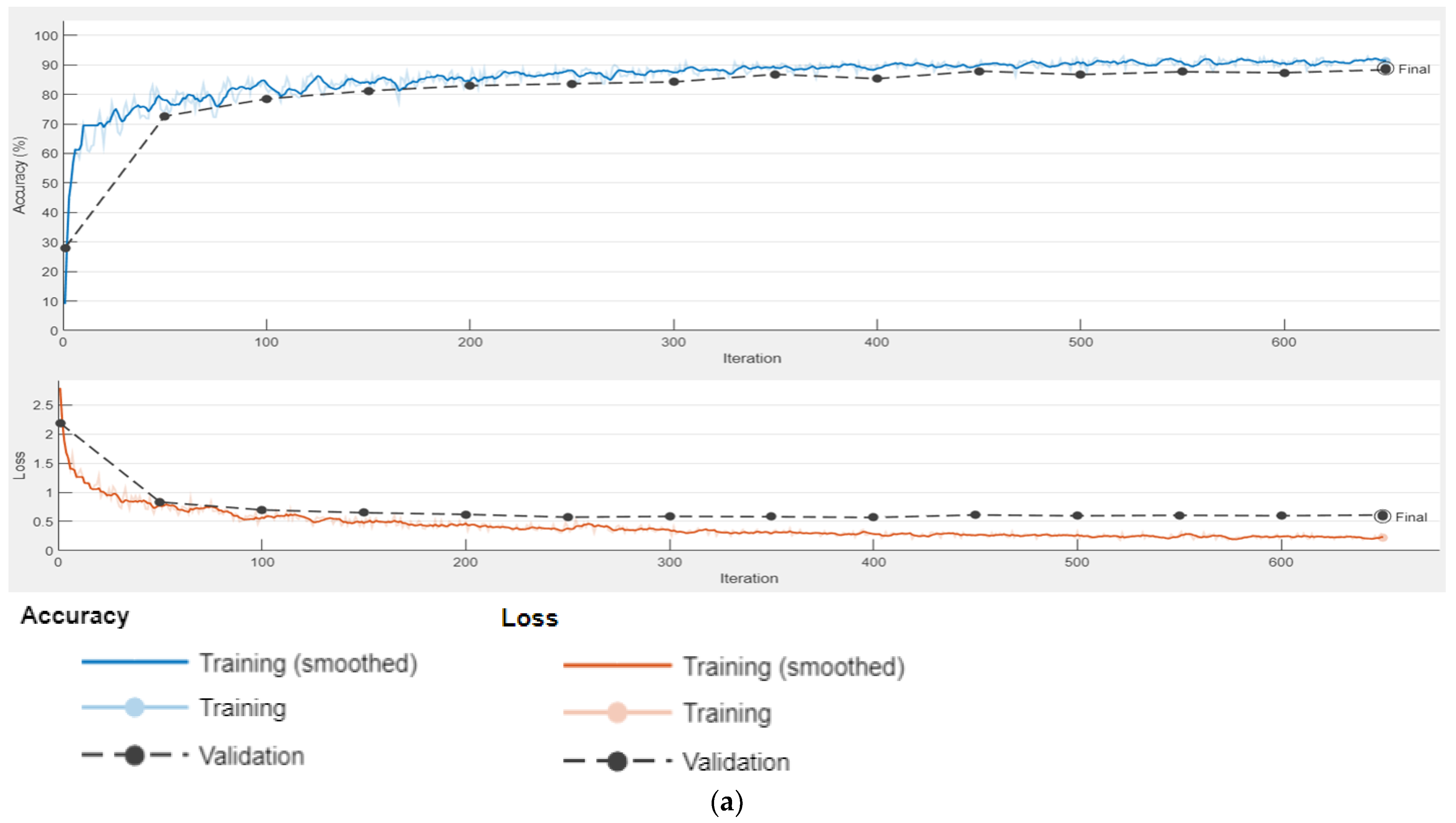
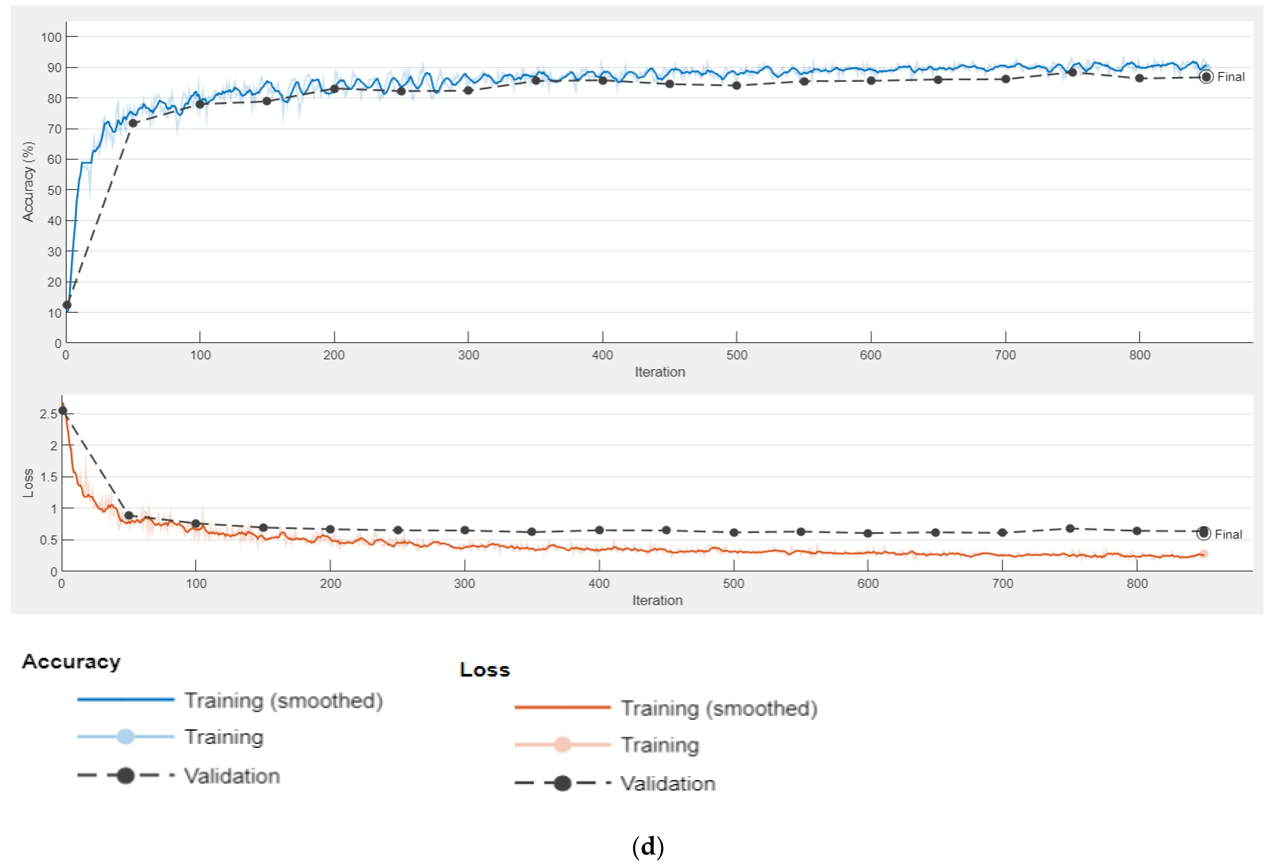
4.2. Implementation Details
4.2.1. Experimental Setup
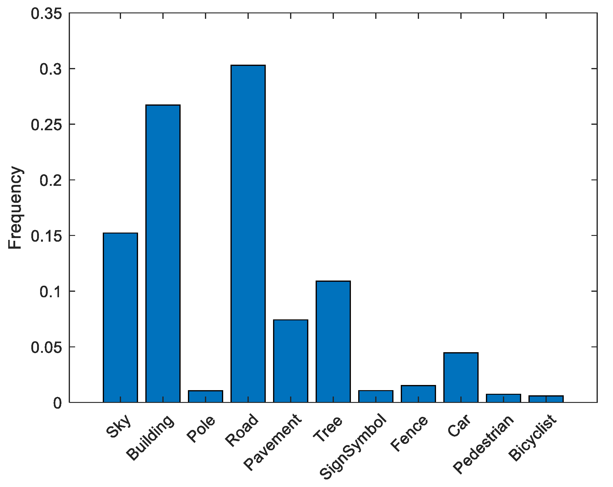
4.2.2. Handling Class Imbalance
4.2.3. Training the Proposed Model Components
Ablation Study
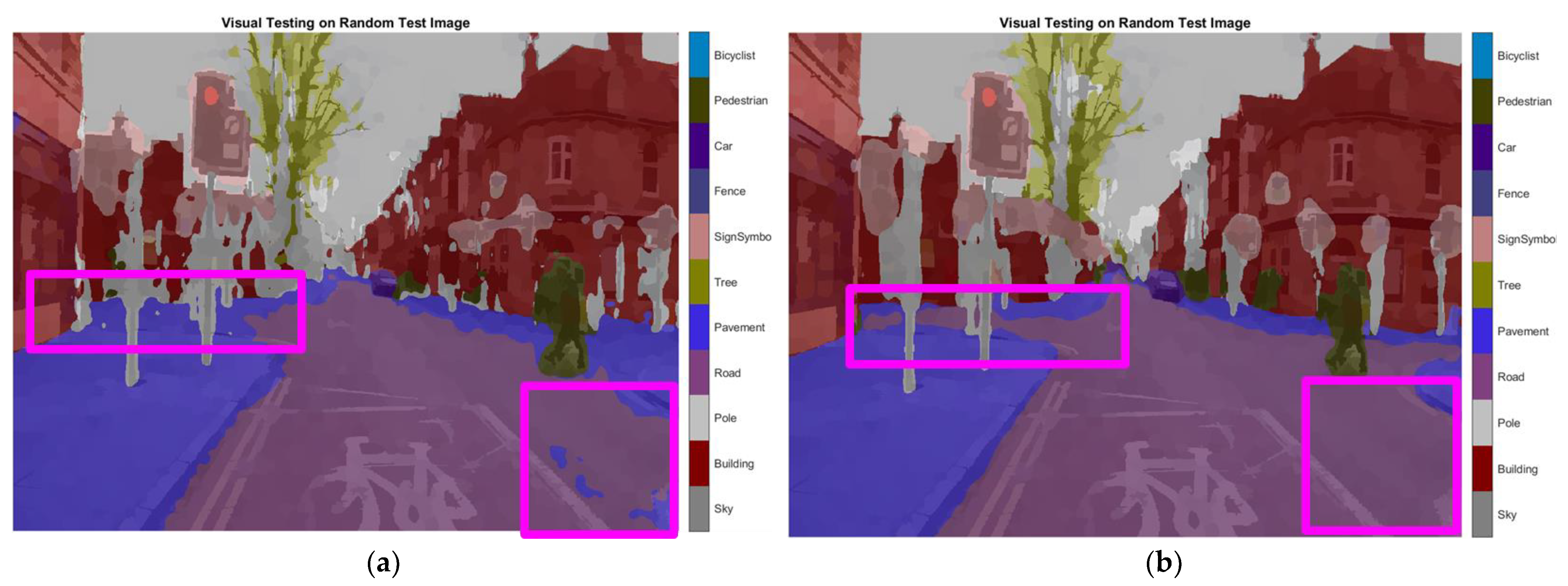
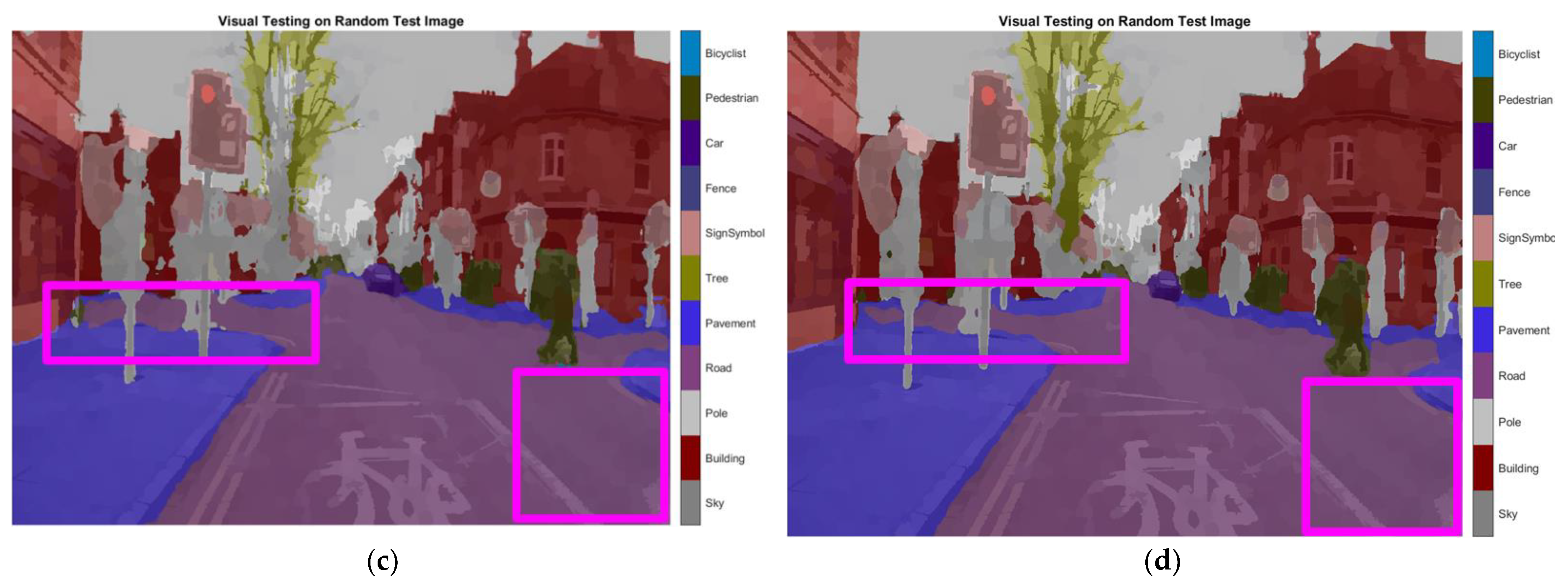
4.3. Comparison with the State-of-the-Art Method
4.4. Semantic Segmentation Analysis Based on
5. Discussion
Novelty and Contributions
- Novel ensemble model approach
- 2.
- Novel semantic segmentation evaluation criterion
6. Conclusions
- (1)
- Preprocessed super-pixeled images, which are locally grouped pixel images that keep track of the local contexts of images;
- (2)
- Non-linear shortcuts followed by group normalization layers in a residual network encoder (ResNet-18) to increase the feature representational power and normalization to ensure improved training accuracy;
- (3)
- A MobileNet-based encoder to increase the depth of the network for fetching fine-grained details using a deeper but less complex network that involves 8.2 million fewer parameters compared with the base ResNet-18 encoder;
- (4)
- A customized pyramid decoder (customized dilated convolution layers) to provide focused control of the receptive field and mitigate the effect of centric exploitations in semi-dark images.
Author Contributions
Funding
Institutional Review Board Statement
Informed Consent Statement
Data Availability Statement
Conflicts of Interest
References
- Memon, M.M.; Hashmani, M.A.; Junejo, A.Z.; Rizvi, S.S.; Arain, A. A Novel Luminance-Based Algorithm for Classification of Semi-Dark Images. Appl. Sci. 2021, 11, 8694. [Google Scholar] [CrossRef]
- Chen, C.; Chen, Q.; Xu, J.; Koltun, V. Learning to see in the dark. In Proceedings of the IEEE Conference on Computer Vision and Pattern Recognition, Salt Lake City, UT, USA, 18–23 June 2018; pp. 3291–3300. [Google Scholar]
- Ouyang, S.; Li, Y. Combining deep semantic segmentation network and graph convolutional neural network for semantic segmentation of remote sensing imagery. Remote Sens. 2021, 13, 119. [Google Scholar] [CrossRef]
- Yu, J.; Zeng, P.; Yu, Y.; Yu, H.; Huang, L.; Zhou, D. A Combined Convolutional Neural Network for Urban Land-Use Classification with GIS Data. Remote Sens. 2022, 14, 1128. [Google Scholar] [CrossRef]
- Senthilnathan, R. Deep Learning in Vision-Based Automated Inspection: Current State and Future Prospects. In Machine Learning in Industry; Springer: Berlin/Heidelberg, Germany, 2022; pp. 159–175. [Google Scholar]
- Chen, L.-C.; Yang, Y.; Wang, J.; Xu, W.; Yuille, A.L. Attention to scale: Scale-aware semantic image segmentation. In Proceedings of the IEEE Conference on Computer Vision and Pattern Recognition, Las Vegas, NV, USA, 27–30 June 2016; pp. 3640–3649. [Google Scholar]
- LeCun, Y.; Bottou, L.; Bengio, Y.; Haffner, P. Gradient-based learning applied to document recognition. Proc. IEEE 1998, 86, 2278–2324. [Google Scholar] [CrossRef] [Green Version]
- Lateef, F.; Ruichek, Y. Survey on semantic segmentation using deep learning techniques. Neurocomputing 2019, 338, 321–348. [Google Scholar] [CrossRef]
- Simonyan, K.; Zisserman, A. Very deep convolutional networks for large-scale image recognition. arXiv 2014, arXiv:1409.1556. [Google Scholar]
- Chen, L.-C.; Papandreou, G.; Kokkinos, I.; Murphy, K.; Yuille, A.L. Deeplab: Semantic image segmentation with deep convolutional nets, atrous convolution, and fully connected crfs. IEEE Trans. Pattern Anal. Mach. Intell. 2018, 40, 834–848. [Google Scholar] [CrossRef] [PubMed] [Green Version]
- Badrinarayanan, V.; Kendall, A.; Cipolla, R. Segnet: A deep convolutional encoder-decoder architecture for image segmentation. IEEE Trans. Pattern Anal. Mach. Intell. 2017, 39, 2481–2495. [Google Scholar] [CrossRef] [PubMed]
- He, K.; Zhang, X.; Ren, S.; Sun, J. Deep residual learning for image recognition. In Proceedings of the IEEE Conference on Computer Vision and Pattern Recognition, Las Vegas, NV, USA, 27–30 June 2016; pp. 770–778. [Google Scholar]
- Chen, L.-C.; Papandreou, G.; Schroff, F.; Adam, H. Rethinking atrous convolution for semantic image segmentation. arXiv 2017, arXiv:1706.05587. [Google Scholar]
- Chen, L.-C.; Zhu, Y.; Papandreou, G.; Schroff, F.; Adam, H. Encoder-decoder with atrous separable convolution for semantic image segmentation. In Proceedings of the European Conference on Computer Vision (ECCV), Munich, Germany, 8–14 September 2018; pp. 801–818. [Google Scholar]
- Zhang, C.; Rameau, F.; Lee, S.; Kim, J.; Benz, P.; Argaw, D.M.; Bazin, J.-C.; Kweon, I.S. Revisiting residual networks with nonlinear shortcuts. In Proceedings of the BMVC, Cardiff, UK, 9–12 September 2019. [Google Scholar]
- McAllister, R.; Gal, Y.; Kendall, A.; Van Der Wilk, M.; Shah, A.; Cipolla, R.; Weller, A. Concrete Problems for Autonomous Vehicle Safety: Advantages of Bayesian Deep Learning. In Proceedings of the Twenty-Sixth International Joint Conference on Artificial Intelligence AI and Autonomy Track, Melbourne, Australia, 19–25 August 2017. [Google Scholar]
- Zhou, X.-Y.; Yang, G.-Z.; Letters, A. Normalization in training U-Net for 2-D biomedical semantic segmentation. IEEE Robot. Autom. Lett. 2019, 4, 1792–1799. [Google Scholar] [CrossRef] [Green Version]
- Zhao, W.; Fu, Y.; Wei, X.; Wang, H. An improved image semantic segmentation method based on superpixels and conditional random fields. Appl. Sci. 2018, 8, 837. [Google Scholar] [CrossRef] [Green Version]
- Zheng, S.; Jayasumana, S.; Romera-Paredes, B.; Vineet, V.; Su, Z.; Du, D.; Huang, C.; Torr, P.H. Conditional random fields as recurrent neural networks. In Proceedings of the IEEE International Conference on Computer Vision, Washington, DC, USA, 7–13 December 2015; pp. 1529–1537. [Google Scholar]
- Plath, N.; Toussaint, M.; Nakajima, S. Multi-class image segmentation using conditional random fields and global classification. In Proceedings of the 26th Annual International Conference on Machine Learning, Montreal, QC, Canada, 14–18 June 2009; pp. 817–824. [Google Scholar]
- Krizhevsky, A.; Sutskever, I.; Hinton, G.E. Imagenet Classification with Deep Convolutional Neural Networks; Association for Computing Machinery: New York, NY, USA, 2012; Volume 25. [Google Scholar]
- Everingham, M.; Eslami, S.; Van Gool, L.; Williams, C.K.; Winn, J.; Zisserman, A. The pascal visual object classes challenge: A retrospective. Int. J. Comput. Vis. 2015, 111, 98–136. [Google Scholar] [CrossRef]
- Lin, T.-Y.; Maire, M.; Belongie, S.; Hays, J.; Perona, P.; Ramanan, D.; Dollár, P.; Zitnick, C.L. Microsoft coco: Common objects in context. In Proceedings of the European Conference on Computer Vision, Zurich, Switzerland, 6–12 September 2014; pp. 740–755. [Google Scholar]
- Cordts, M.; Omran, M.; Ramos, S.; Rehfeld, T.; Enzweiler, M.; Benenson, R.; Franke, U.; Roth, S.; Schiele, B. The cityscapes dataset for semantic urban scene understanding. In Proceedings of the IEEE Conference on Computer Vision and Pattern Recognition, Las Vegas, NV, USA, 27–30 June 2016; pp. 3213–3223. [Google Scholar]
- Brostow, G.J.; Fauqueur, J.; Cipolla, R.J.P.R.L. Semantic object classes in video: A high-definition ground truth database. Pattern Recognit. Lett. 2009, 30, 88–97. [Google Scholar] [CrossRef]
- Song, S.; Lichtenberg, S.P.; Xiao, J. Sun rgb-d: A rgb-d scene understanding benchmark suite. In Proceedings of the IEEE Conference on Computer Vision and Pattern Recognition, Boston, MA, USA, 7–12 June 2015; pp. 567–576. [Google Scholar]
- Cogswell, M.; Lin, X.; Purushwalkam, S.; Batra, D. Combining the best of graphical models and convnets for semantic segmentation. arXiv 2014, arXiv:1412.4313. [Google Scholar]
- Farabet, C.; Couprie, C.; Najman, L.; LeCun, Y. Learning hierarchical features for scene labeling. IEEE Trans. Pattern Anal. Mach. Intell. 2012, 35, 1915–1929. [Google Scholar] [CrossRef] [PubMed] [Green Version]
- Liu, C.; Yuen, J.; Torralba, A.; Sivic, J.; Freeman, W.T. Sift flow: Dense correspondence across different scenes. In Proceedings of the European Conference on Computer Vision, Marseille, France, 12–18 October 2008; pp. 28–42. [Google Scholar]
- Tighe, J.; Lazebnik, S. Superparsing: Scalable nonparametric image parsing with superpixels. In Proceedings of the European Conference on Computer Vision, Heraklion, Greece, 5–11 September 2010; pp. 352–365. [Google Scholar]
- Gould, S.; Fulton, R.; Koller, D. Decomposing a scene into geometric and semantically consistent regions. In Proceedings of the 2009 IEEE 12th International Conference on Computer Vision, Kyoto, Japan, 27 September–4 October 2009; pp. 1–8. [Google Scholar]
- Papandreou, G.; Chen, L.-C.; Murphy, K.P.; Yuille, A.L. Weakly-and semi-supervised learning of a deep convolutional network for semantic image segmentation. In Proceedings of the IEEE International Conference on Computer Vision, Santiago, Chile, 7–13 December 2015; pp. 1742–1750. [Google Scholar]
- Saito, S.; Kerola, T.; Tsutsui, S. Superpixel Clustering with Deep Features for Unsupervised Road Segmentation. 2017. Available online: https://www.arxiv-vanity.com/papers/1711.05998/ (accessed on 29 May 2022).
- He, Y.; Chiu, W.-C.; Keuper, M.; Fritz, M. Std2p: Rgbd semantic segmentation using spatio-temporal data-driven pooling. In Proceedings of the IEEE Conference on Computer Vision and Pattern Recognition, Honolulu, HI, USA, 21–26 July 2017; pp. 4837–4846. [Google Scholar]
- Zhou, L.; Fu, K.; Liu, Z.; Zhang, F.; Yin, Z.; Zheng, J.J.N. Superpixel based continuous conditional random field neural network for semantic segmentation. Neurocomputing 2019, 340, 196–210. [Google Scholar] [CrossRef]
- Kae, A.; Sohn, K.; Lee, H.; Learned-Miller, E. Augmenting CRFs with Boltzmann machine shape priors for image labeling. In Proceedings of the IEEE Conference on Computer Vision and Pattern Recognition, Portland, OR, USA, 23–28 June 2013; pp. 2019–2026. [Google Scholar]
- Smith, B.M.; Zhang, L.; Brandt, J.; Lin, Z.; Yang, J. Exemplar-based face parsing. In Proceedings of the IEEE conference on Computer Vision and Pattern Recognition, Portland, OR, USA, 23–28 June 2013; pp. 3484–3491. [Google Scholar]
- Fisher Yu, V.K. Multi-Scale Context Aggregation by Dilated Convolutions. arXiv 2015, arXiv:1511.07122. [Google Scholar]
- Wu, Y.; He, K. Group normalization. In Proceedings of the European Conference on Computer Vision (ECCV), Munich, Germany, 8–14 September 2018; pp. 3–19. [Google Scholar]
- Dumoulin, V.; Visin, F. A guide to convolution arithmetic for deep learning. arXiv 2016, arXiv:1603.07285. [Google Scholar]
- Brostow, G.J.; Shotton, J.; Fauqueur, J.; Cipolla, R. Segmentation and recognition using structure from motion point clouds. In Proceedings of the European Conference on Computer Vision, Marseille, France, 12–18 October 2008; pp. 44–57. [Google Scholar]
- Csurka, G.; Larlus, D.; Perronnin, F.; Meylan, F.J.I.P. What is a good evaluation measure for semantic segmentation? In Proceedings of the British Machine Vision Conference; BMVA Press: London, UK, 2013; Volume 26. [Google Scholar]
- Fernandez-Moral, E.; Martins, R.; Wolf, D.; Rives, P. A new metric for evaluating semantic segmentation: Leveraging global and contour accuracy. In Proceedings of the 2018 IEEE Intelligent Vehicles Symposium (iv), Suzhou, China, 26–30 June 2018; pp. 1051–1056. [Google Scholar]
- Saito, M.; Matsumoto, M. SIMD-oriented fast Mersenne Twister: A 128-bit pseudorandom number generator. In Monte Carlo and Quasi-Monte Carlo Methods 2006; Springer: Berlin/Heidelberg, Germany, 2008; pp. 607–622. [Google Scholar]


| Deep Learning Architecture | Original Architecture | Testing Benchmark | Semi-Dark Image Handling | Observations |
|---|---|---|---|---|
| VGG [9] | AlexNet [21] | ILSVRC-2012 Pascal VOC [22] MS Coco [23] | 🗙 | |
| ResNet [12] | VGG [9] | ILSVRC-2012 | 🗙 |
|
| Pascal VOC [22] MS Coco [23] | ||||
| DeepLab [10] | VGG [9] | Pascal VOC [22] Cityscapes [24] | 🗙 |
|
| SegNet [11] | VGG [9] | Cam Vid Dataset [25] Sun RGB-D [26] | ✓ |
|
| DeepLabV2 [10] | VGG [9] | Pascal VOC [22] MS Coco [23] Cityscapes [24] | 🗙 |
|
| DeepLabV3 [13] | DeepLabV2 [10] | Pascal VOC [22] Cityscapes [24] | 🗙 |
|
| DeepLabV3+ [14] | DeepLabV3 [13], ResNet [12] | Pascal VOC [22] Cityscapes [24] | 🗙 |
|
| Attention Model [6] | Super-pixel creation (SLIC) DeepLab [10] | Pascal VOC [22] MS Coco [23] | 🗙 |
|
| Super-Pixel and CRF-Based FCN [18] | Cityscapes [24] | 🗙 |
| |
| Super-Pixel-Based Hierarchical Network [28] | Super-pixel creation (tree/clustering) ConvNet (2-layer MLP) CRF | SIFT Flow dataset [29] Barcelona dataset [30] Stanford background [31] | 🗙 |
|
| Semi-Supervised Convolution Neural Network [32] | DeepLab-CRF [10] | Pascal VOC [22] MS Coco [23] | 🗙 |
|
| Higher-Order CRF in DNN | FCN VGG [9] | Pascal VOC [22] | 🗙 |
|
| Super-Pixel-Based DCNN for Road Segmentation [33] | VGG [9], ResNet [12] | Cityscapes [24] | 🗙 |
|
| Super-Pixel and Statistically Learned DCNN | Simple fully convolution neural network | Pascal VOC [22] Sun RGB-D [26] | ✓ |
|
| Spatio-Temporal Data-Driven Pooling DCNN [34] | CNN (No specifics written) | Sun RGB-D [26] | ✓ |
|
| Super-Pixel- and CRF-Based DCNN [35] | SEGNET-VGG16 [11], DeepLabV2-ResNet [10] | LFW-PL dataset [36], HELEN dataset [37] (facial images) Pascal VOC [22] | 🗙 |
|
| S# | Merged Class | Actual CamVid Dataset Class |
|---|---|---|
| 1 | Sky | Sky |
| 2 | Building | Bridge Building Wall Tunnel Archway |
| 3 | Pole | Column_Pole TrafficCone |
| 4 | Road | Road LaneMkgsDriv LaneMkgsNonDriv |
| 5 | Pavement | Sidewalk ParkingBlock RoadShoulder |
| 6 | Tree | Tree VegetationMisc |
| 7 | Sign Symbol | SignSymbol Misc_Text TrafficLight |
| 8 | Fence | Fence |
| 9 | Car | Car SUVPickupTruck Truck_Bus Train OtherMoving |
| 10 | Pedestrian | Pedestrian Child CartLuggagePram Animal |
| 11 | Bicyclist | Bicyclist MotorcycleScooter |
| Sample 1 | Sample 2 | Sample 3 | Sample 4 | Sample 5 | |
|---|---|---|---|---|---|
| Images | 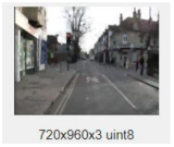 |  |  | 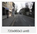 | 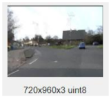 |
| Ground truth | 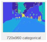 |  | 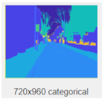 | 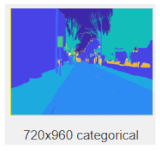 | 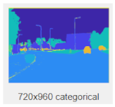 |
| Parameter | Solver | Initial Learning Rate | Validation Frequency | Maximum Epochs | Mini-Batch Size | L2 Regularization | Gradient Threshold Method | Validation Patience | Shuffle |
|---|---|---|---|---|---|---|---|---|---|
| Value | Sgdm (Stochastic Gradient Descent with Momentum) | 0.01 | 50 | 25 | 8 | 0.0001 | L2 Norm | 5 | Every-epoch |
| Class | Weight Value |
|---|---|
| Sky | 0.2933 |
| Building | 0.1674 |
| Pole | 4.2693 |
| Road | 0.1480 |
| Pavement | 0.5942 |
| Tree | 0.3766 |
| Sign Symbol | 4.0753 |
| Fence | 1.5294 |
| Car | 1.0000 |
| Pedestrian | 5.6283 |
| Bicyclist | 4.2795 |
| Network | Class | Sky | Building | Pole | Road | Pavement | Tree | Sign Symbol | Fence | Car | Pedestrian | Bicyclist | Average | |
|---|---|---|---|---|---|---|---|---|---|---|---|---|---|---|
| Metrics | ||||||||||||||
| RGSNet-DeepLab | OA | 0.9408 | 0.7491 | 0.5761 | 0.9241 | 0.9028 | 0.8509 | 0.8152 | 0.7119 | 0.8612 | 0.8506 | 0.8001 | 0.8166 | |
| IoU | 0.9046 | 0.7223 | 0.1657 | 0.9161 | 0.6983 | 0.7502 | 0.2220 | 0.5180 | 0.7009 | 0.2914 | 0.5184 | 0.5825 | ||
| Mean BFScore | 0.8723 | 0.5457 | 0.4613 | 0.7616 | 0.6879 | 0.6343 | 0.3308 | 0.4337 | 0.6020 | 0.4452 | 0.4675 | 0.5675 | ||
| 0.9066 | 0.6475 | 0.5183 | 0.8429 | 0.7952 | 0.7426 | 0.5726 | 0.57278 | 0.7316 | 0.6475 | 0.6336 | 0.6919 | |||
| MobileNet-DeepLab | OA | 0.9640 | 0.7621 | 0.6752 | 0.9516 | 0.8901 | 0.8523 | 0.7258 | 0.7337 | 0.8819 | 0.7703 | 0.7852 | 0.8175 | |
| IoU | 0.9128 | 0.7343 | 0.1605 | 0.9378 | 0.7405 | 0.7474 | 0.3064 | 0.5638 | 0.7315 | 0.3551 | 0.5997 | 0.6173 | ||
| Mean BFScore | 0.9015 | 0.5374 | 0.4609 | 0.8305 | 0.7510 | 0.6375 | 0.4291 | 0.5046 | 0.6489 | 0.5114 | 0.5943 | 0.6188 | ||
| 0.9327 | 0.6498 | 0.5676 | 0.8911 | 0.8205 | 0.7449 | 0.5772 | 0.6191 | 0.7653 | 0.6405 | 0.6896 | 0.7180 | |||
| Customized Decoder-DeepLab | OA | 0.9498 | 0.8438 | 0.6427 | 0.9519 | 0.8695 | 0.8899 | 0.6828 | 0.7604 | 0.8942 | 0.7739 | 0.8127 | 0.8247 | |
| IoU | 0.9124 | 0.8047 | 0.2115 | 0.9383 | 0.7484 | 0.7760 | 0.3663 | 0.6091 | 0.7558 | 0.4198 | 0.5922 | 0.6486 | ||
| Mean BFScore | 0.8913 | 0.6405 | 0.5579 | 0.8295 | 0.7706 | 0.6858 | 0.4914 | 0.5272 | 0.6834 | 0.6007 | 0.6179 | 0.6633 | ||
| 0.9205 | 0.7422 | 0.5999 | 0.8907 | 0.8199 | 0.7878 | 0.5868 | 0.6437 | 0.7887 | 0.6870 | 0.7151 | 0.7438 | |||
| Test Case | Network | |||
|---|---|---|---|---|
| ResNet-DeepLabV3+ | RGSNet-DeepLab | MobileNet-DeepLab | Customized Decoder-DeepLab | |
| 1 | 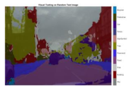 |  |  |  |
| 2 |  |  |  | 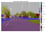 |
| 3 | 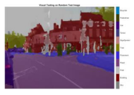 | 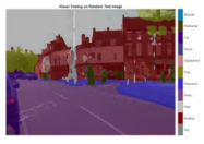 |  | 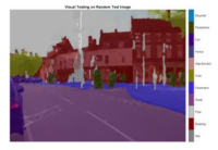 |
| 4 | 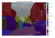 | 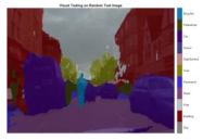 |  | 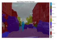 |
| Network | Class | Sky | Building | Pole | Road | Pavement | Tree | Sign Symbol | Fence | Car | Pedestrian | Bicyclist | Average | |
|---|---|---|---|---|---|---|---|---|---|---|---|---|---|---|
| Metrics | ||||||||||||||
| ResNet-DeepLabV3+ | OA | 0.9486 | 0.8418 | 0.6557 | 0.9536 | 0.8779 | 0.8533 | 0.6782 | 0.7724 | 0.8812 | 0.8064 | 0.8261 | 0.8268 | |
| IoU | 0.9100 | 0.7976 | 0.1938 | 0.9406 | 0.7536 | 0.7625 | 0.399 | 0.5736 | 0.7402 | 0.3970 | 0.5937 | 0.6420 | ||
| Mean BFScore | 0.8942 | 0.6253 | 0.5299 | 0.8348 | 0.7779 | 0.6674 | 0.5191 | 0.4978 | 0.6567 | 0.5621 | 0.5778 | 0.6494 | ||
| 0.9214 | 0.7336 | 0.5923 | 0.8942 | 0.8278 | 0.7603 | 0.5984 | 0.6350 | 0.7689 | 0.6839 | 0.7018 | 0.7380 | |||
| Unified DeepLab | OA | 0.9640 | 0.8438 | 0.6752 | 0.9519 | 0.9028 | 0.8899 | 0.8152 | 0.7604 | 0.8942 | 0.8506 | 0.8127 | 0.8510 | |
| IoU | 0.9128 | 0.8047 | 0.2115 | 0.9383 | 0.7484 | 0.7760 | 0.3663 | 0.6091 | 0.7558 | 0.4198 | 0.5997 | 0.6493 | ||
| Mean BFScore | 0.9015 | 0.6405 | 0.5579 | 0.8305 | 0.7706 | 0.6858 | 0.4914 | 0.5272 | 0.6834 | 0.6007 | 0.6179 | 0.6643 | ||
| 0.9327 | 0.7422 | 0.6161 | 0.8912 | 0.8366 | 0.7878 | 0.6530 | 0.6437 | 0.7887 | 0.7253 | 0.7151 | 0.7575 | |||
| Network | |||
|---|---|---|---|
| ResNet-DeepLabV3+ | Incremental MeanBFScore | 64 = 0, = 0, = 1 | 72.99 = 0.4995, = 0.4995, = 0.001 |
| Unified DeepLab | Incremental MeanBFScore | 66 = 0, = 0, = 1 | 74.49 = 0.4995, = 0.4995, = 0.001 |
| ResNet-DeepLabV3+ | Incremental IoU | 64 = 0, = 1, = 0 | 72.99 W1 = 0.4995, = 0.001, = 0.4995 |
| Unified DeepLab | Incremental IoU | 64 = 0, = 1, = 0 | 75.48 = 0.4995, = 0.001, = 0.4995 |
| ResNet-DeepLabV3+ | Incremental OA | 64.02 = 0.0010, = 0.4995, = 0.4995 | 82 = 1, = 0, = 0 |
| Unified DeepLab | Incremental OA | 65.02 = 0.0010, = 0.4995, = 0.4995 | 85 = 1, = 0, = 0 |
| ResNet-DeepLabV3+ | Randomized | 64.00 = 0.00008, = 0.48808, = 0.51184 | 69.38 = 0.29931, = 0.51779, = 0.18290 |
| Unified DeepLab | Randomized | 64.97 = 0.00863, = 0.59849, = 0.39288 | 71.02 = 0.2993822, = 0.33354, = 0.36708 |
Publisher’s Note: MDPI stays neutral with regard to jurisdictional claims in published maps and institutional affiliations. |
© 2022 by the authors. Licensee MDPI, Basel, Switzerland. This article is an open access article distributed under the terms and conditions of the Creative Commons Attribution (CC BY) license (https://creativecommons.org/licenses/by/4.0/).
Share and Cite
Memon, M.M.; Hashmani, M.A.; Junejo, A.Z.; Rizvi, S.S.; Raza, K. Unified DeepLabV3+ for Semi-Dark Image Semantic Segmentation. Sensors 2022, 22, 5312. https://doi.org/10.3390/s22145312
Memon MM, Hashmani MA, Junejo AZ, Rizvi SS, Raza K. Unified DeepLabV3+ for Semi-Dark Image Semantic Segmentation. Sensors. 2022; 22(14):5312. https://doi.org/10.3390/s22145312
Chicago/Turabian StyleMemon, Mehak Maqbool, Manzoor Ahmed Hashmani, Aisha Zahid Junejo, Syed Sajjad Rizvi, and Kamran Raza. 2022. "Unified DeepLabV3+ for Semi-Dark Image Semantic Segmentation" Sensors 22, no. 14: 5312. https://doi.org/10.3390/s22145312
APA StyleMemon, M. M., Hashmani, M. A., Junejo, A. Z., Rizvi, S. S., & Raza, K. (2022). Unified DeepLabV3+ for Semi-Dark Image Semantic Segmentation. Sensors, 22(14), 5312. https://doi.org/10.3390/s22145312