
Localization of Dielectric Anomalies with Multi-Monostatic S11 Using 2D MUSIC Algorithm with Spatial Smoothing


Abstract
:1. Introduction
- (1)
- (2)
- (3)
- TD systems tend to offer faster scan times and lower costs of measurement devices [5].
2. Mathematical Model
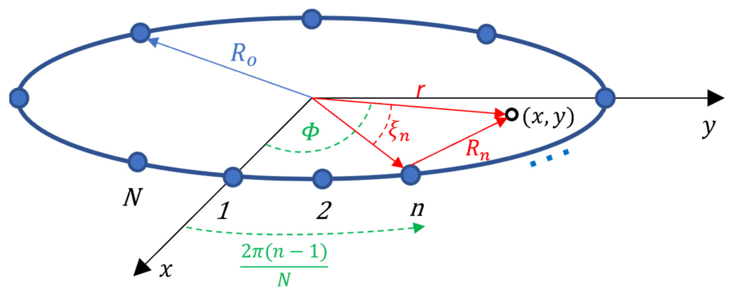
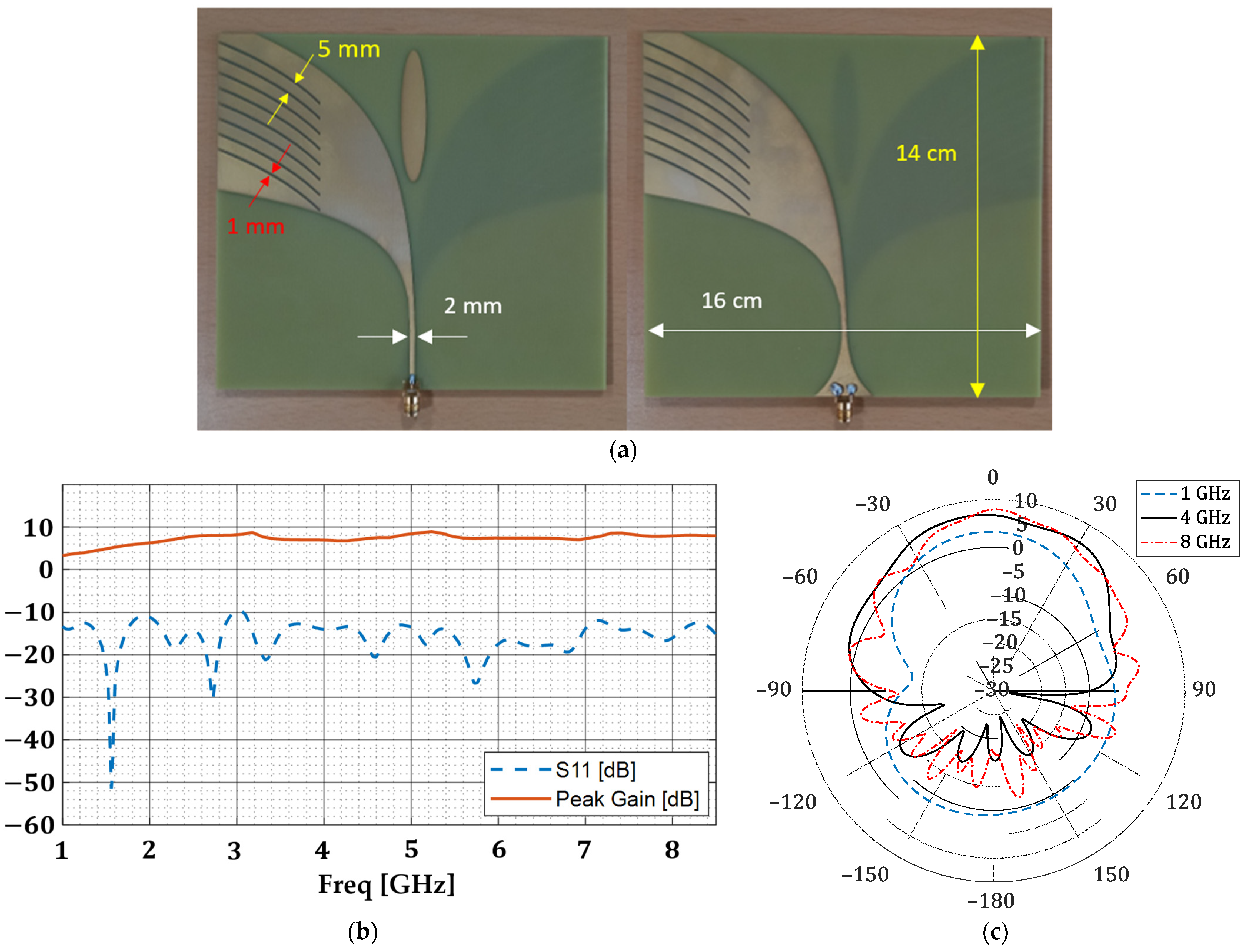
2.1. Near-Field ISAR Imaging
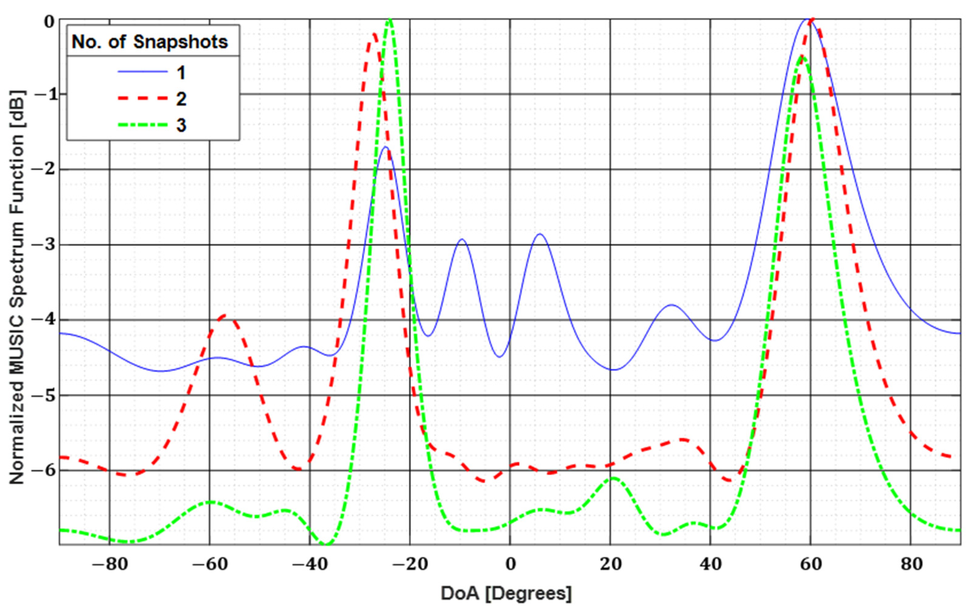
2.2. Near-Field ISAR Imaging with Spatial Smoothing
| Algorithm 1: 2D MUSIC with Spatial Smoothing | ||||
| Input: Complex matrix of size M × N as shown in Equation (13) | ||||
| Output: Near-field ISAR image with target location | ||||
| 1 | Compute kx and ky using frequencies and angles; | |||
| 2 | Translate E(km, Φn) to E(kx, ky) using polar to cartesian transformation; | |||
| 3 | Compute Ê(kx, ky) using Equation (12); | |||
| 4 | Rearrange into sub-arrays using Equation (14); | |||
| 5 | Compute Cxx using Equation (15) and construct matrix Z whose columns are the eigenvectors of Cxx corresponding to eigenvalues that are smaller than the threshold d; | |||
| 6 | foreach sub-array | |||
| 7 | foreach pixel | |||
| 8 | Initialize steering vector a(x, y); | |||
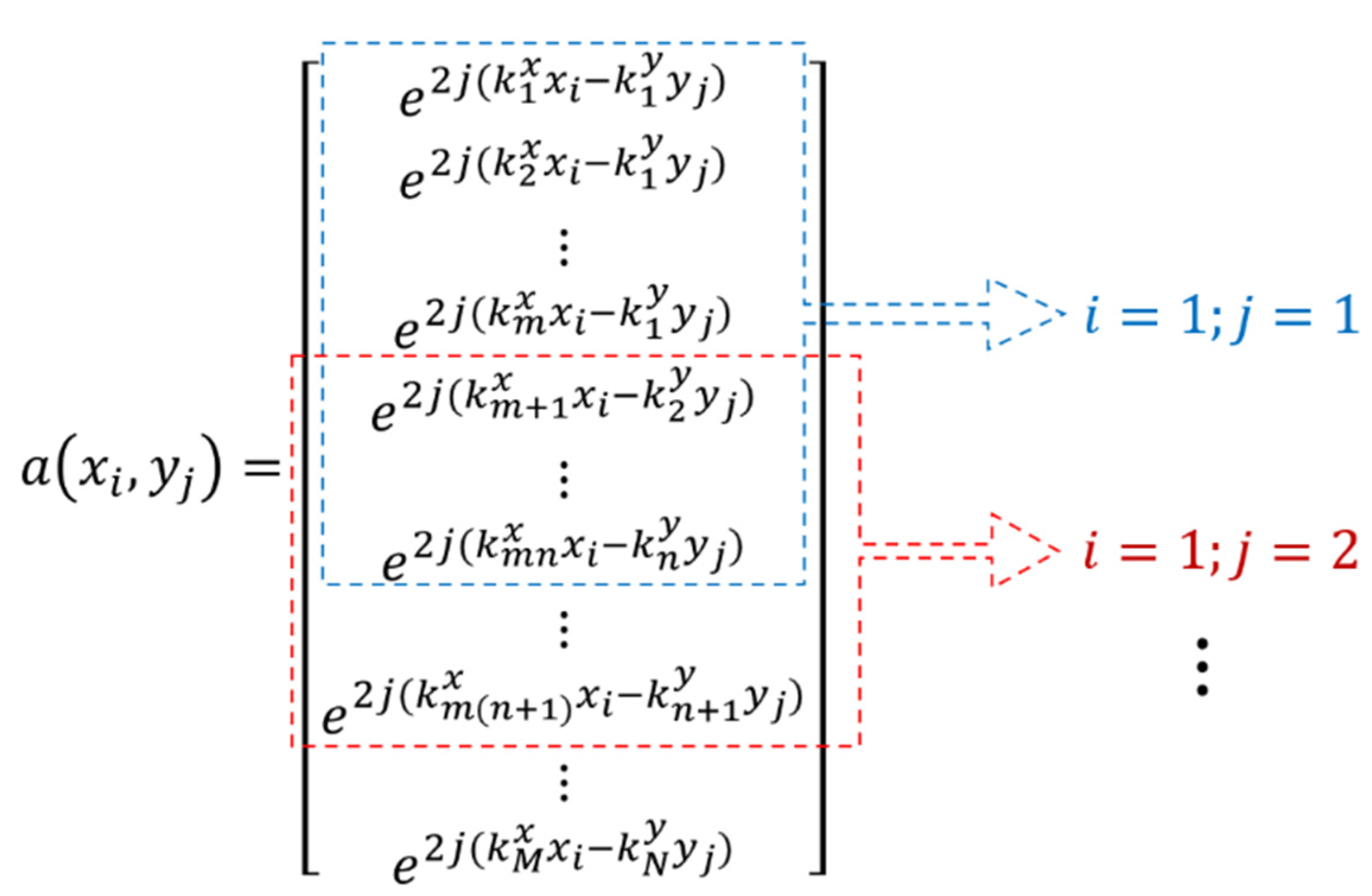
| 9 | Fill a(x, y) with corresponding entries according to Figure 6; | |||
| 10 | Compute image pixel using Z and a(x, y) in Equation (11); | |||
| 11 | end | |||
| 12 | end | |||
| 13 | PlotPMUSIC(x, y) | |||
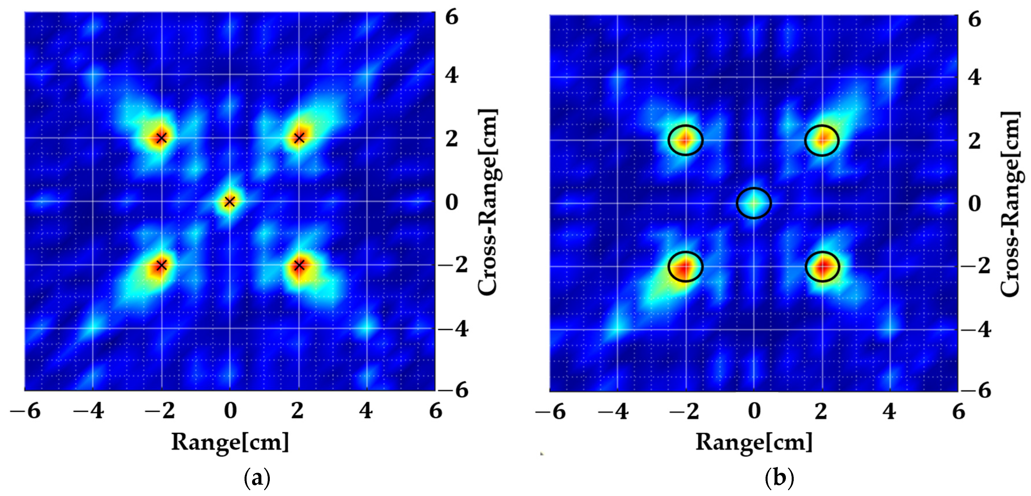
3. Simulation
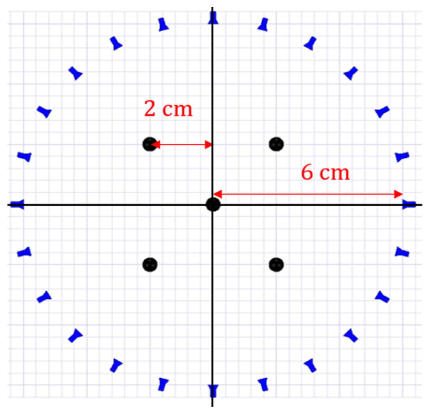
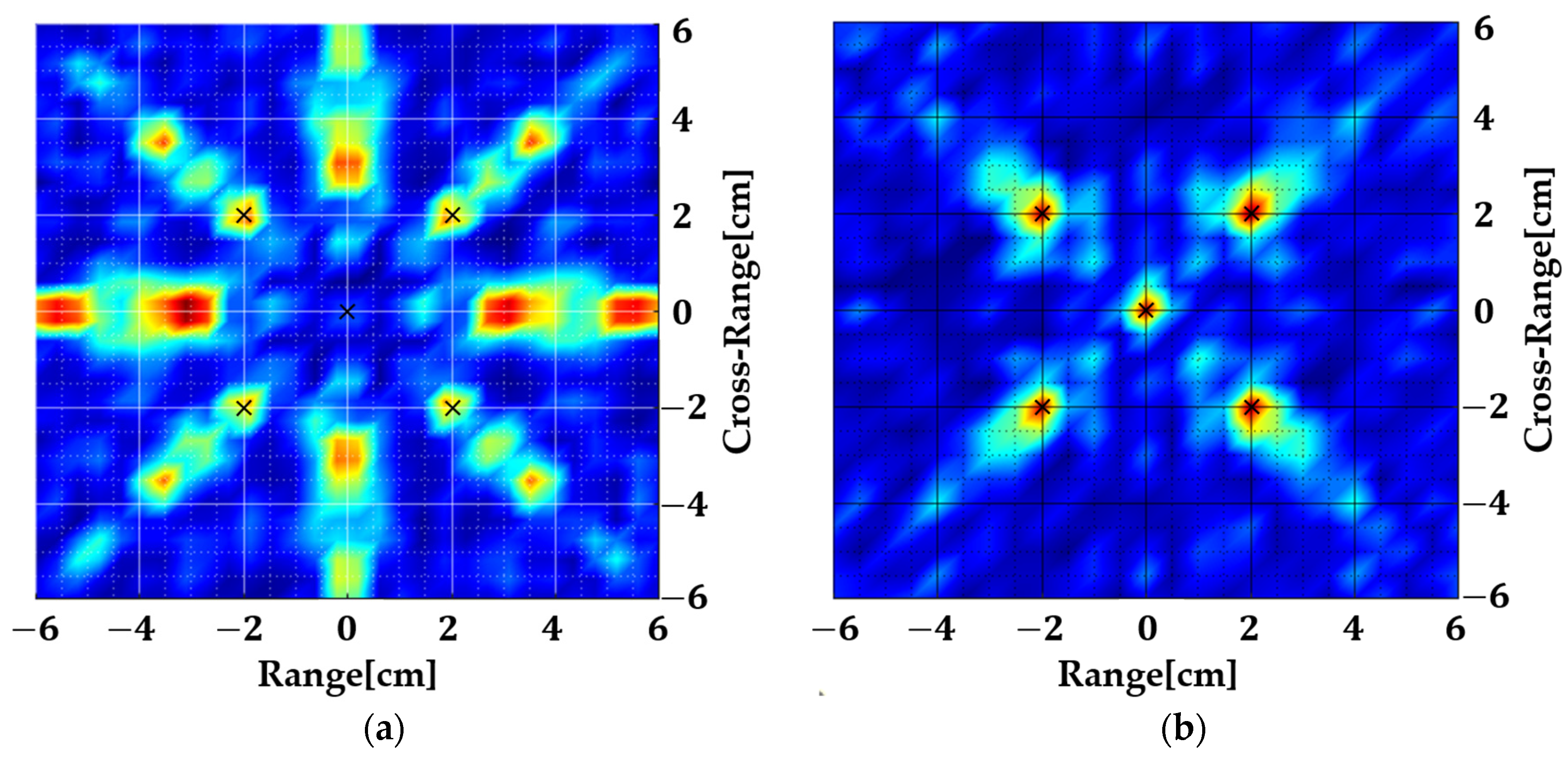
3.1. Using Scattered Field in Near-Region
3.2. Using Scattering Parameter
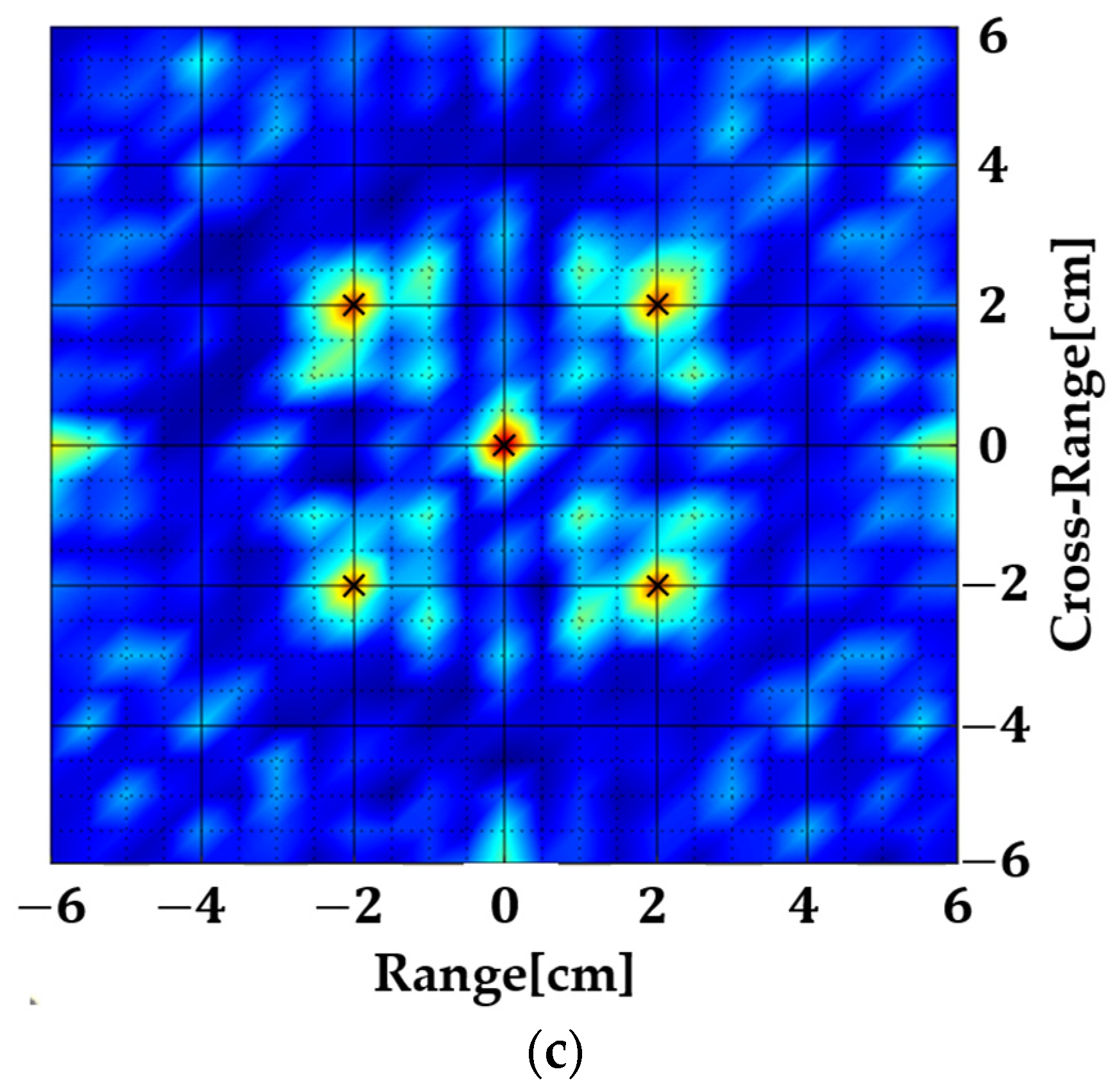
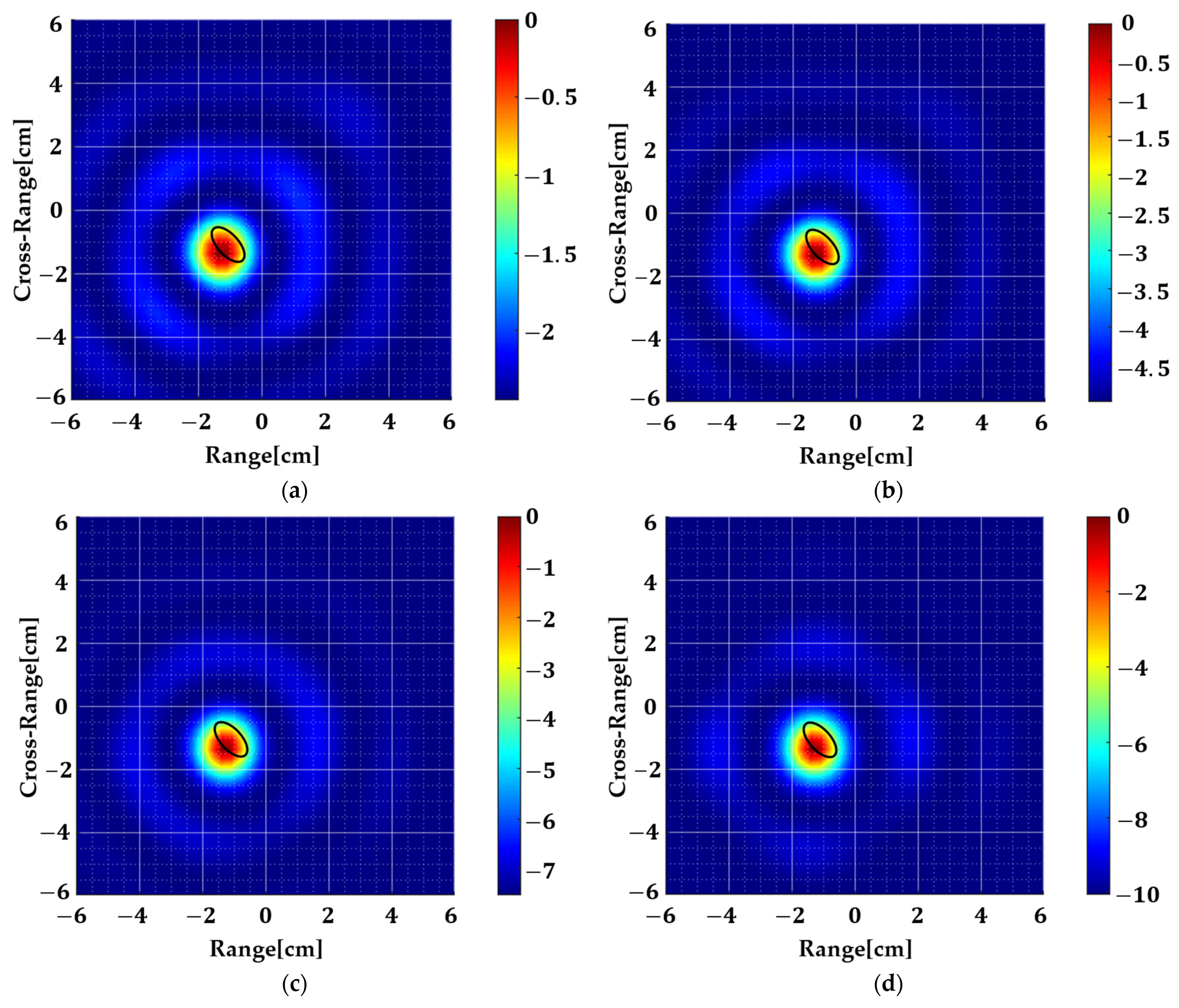
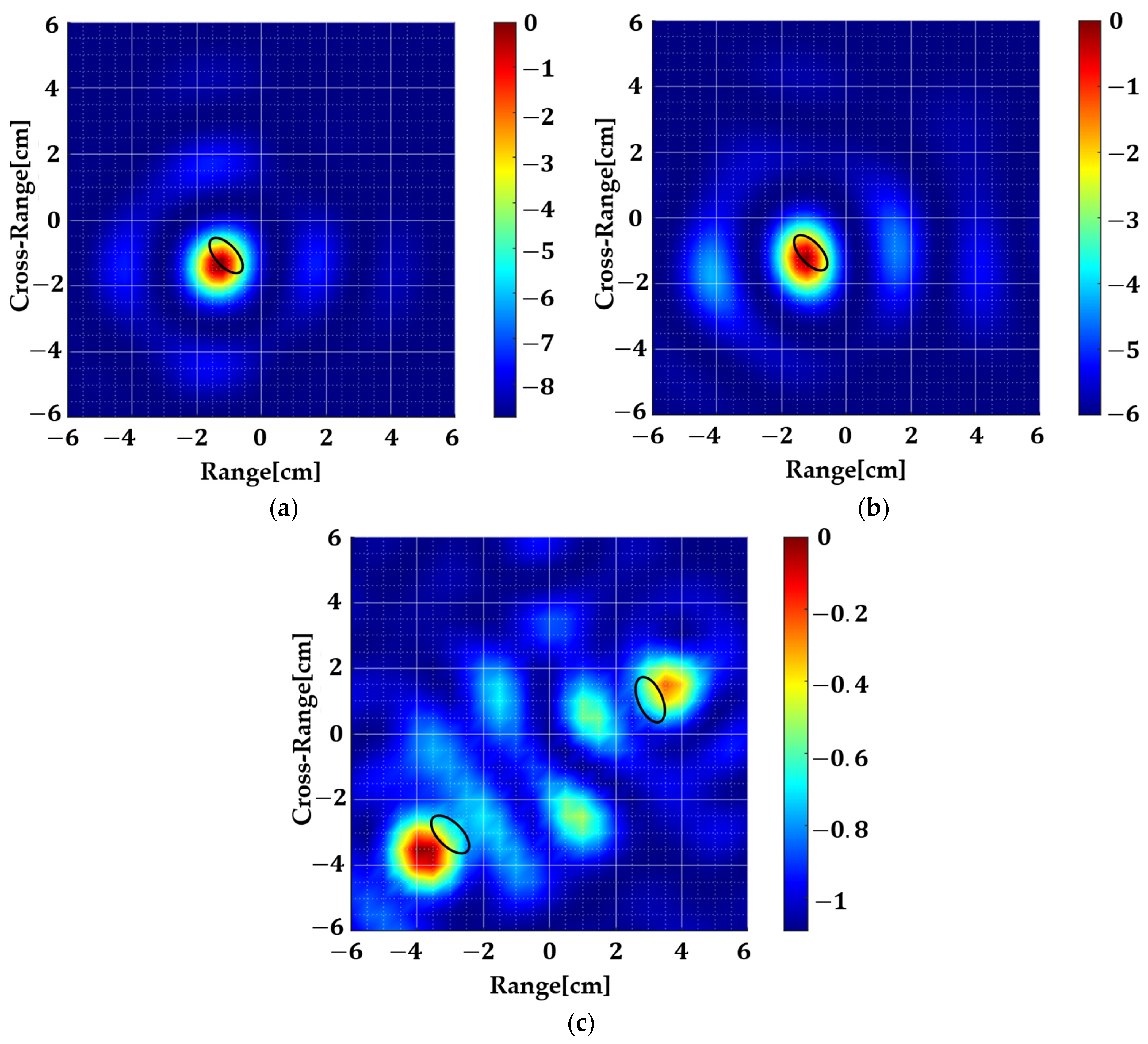
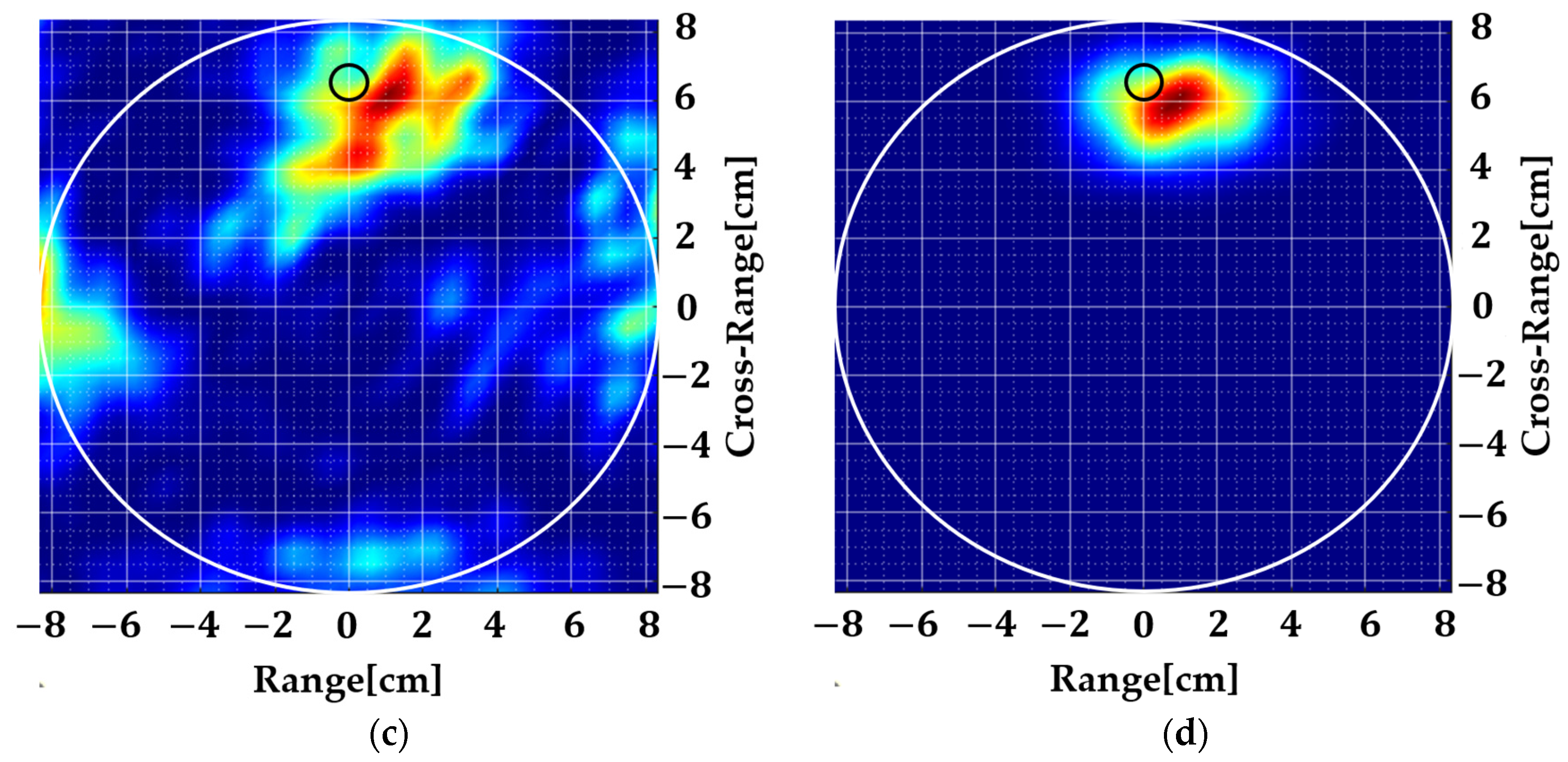
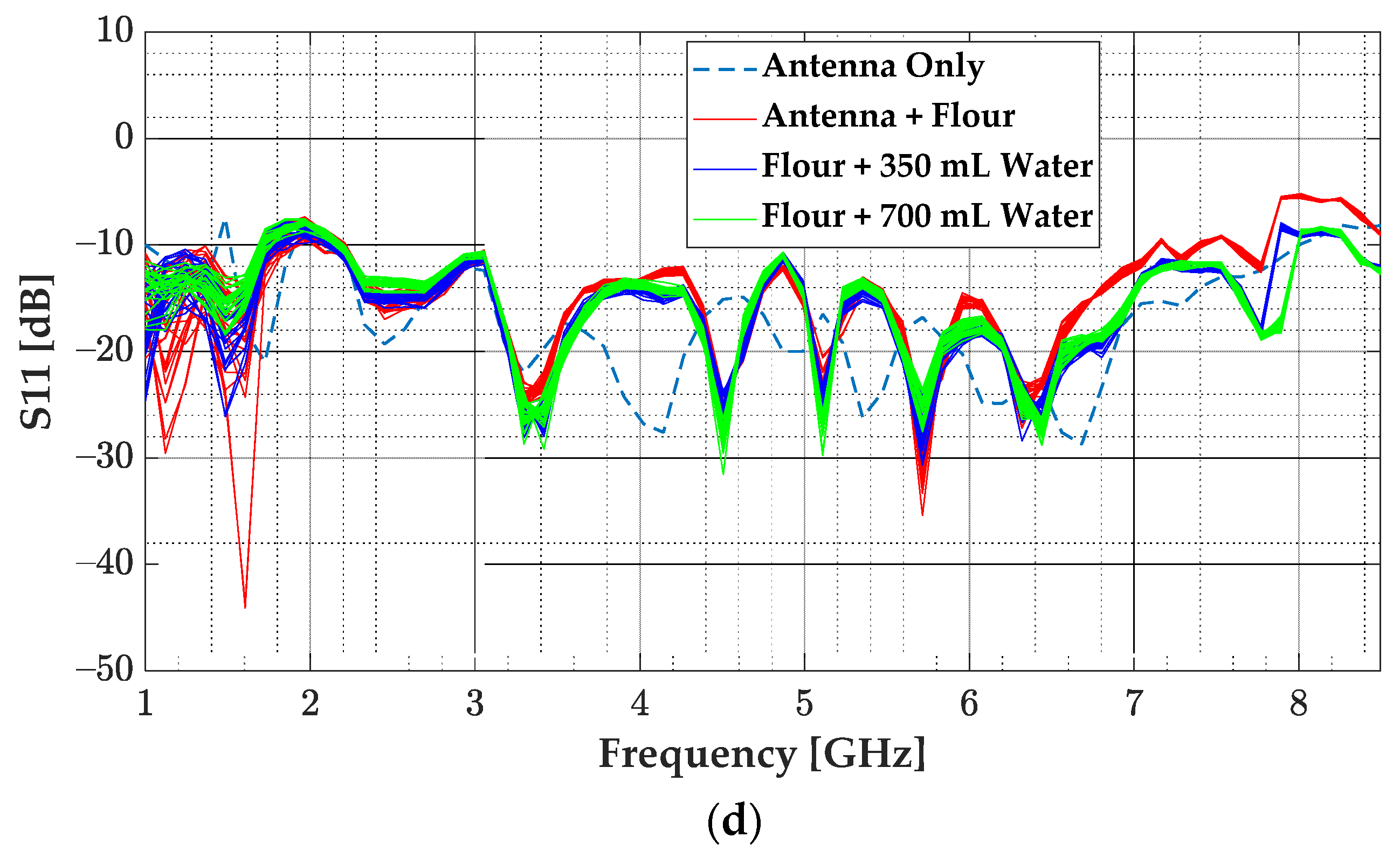
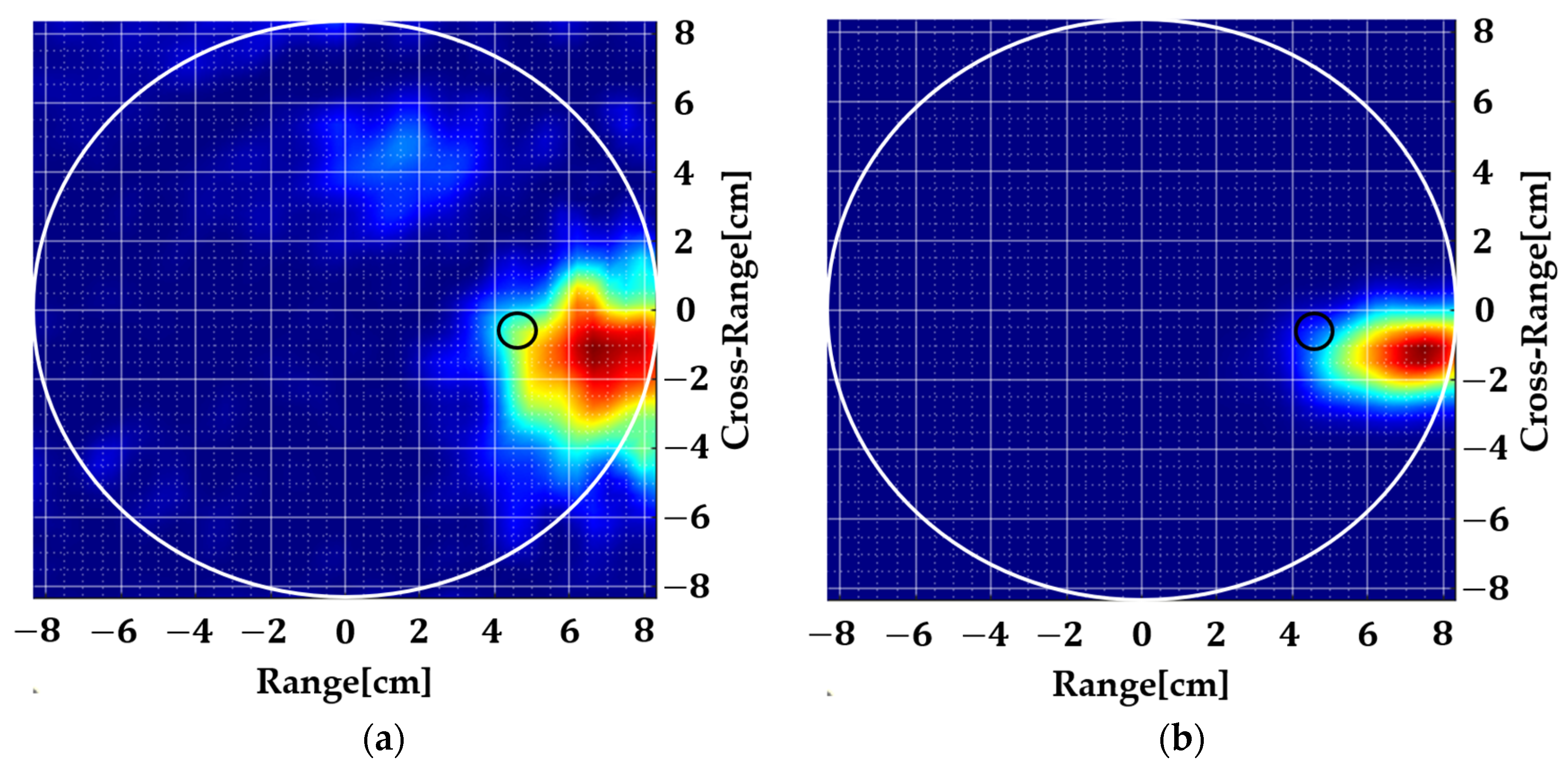
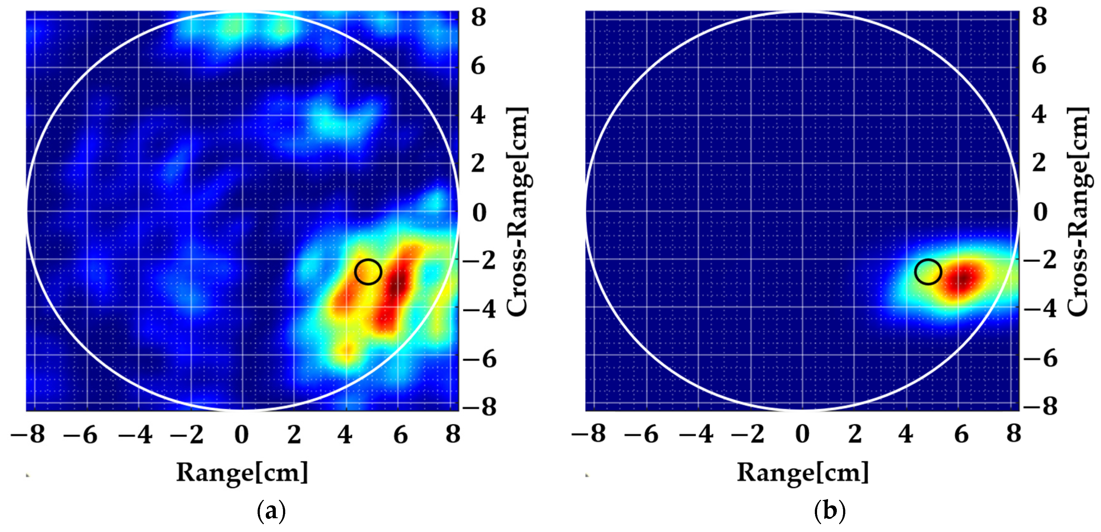
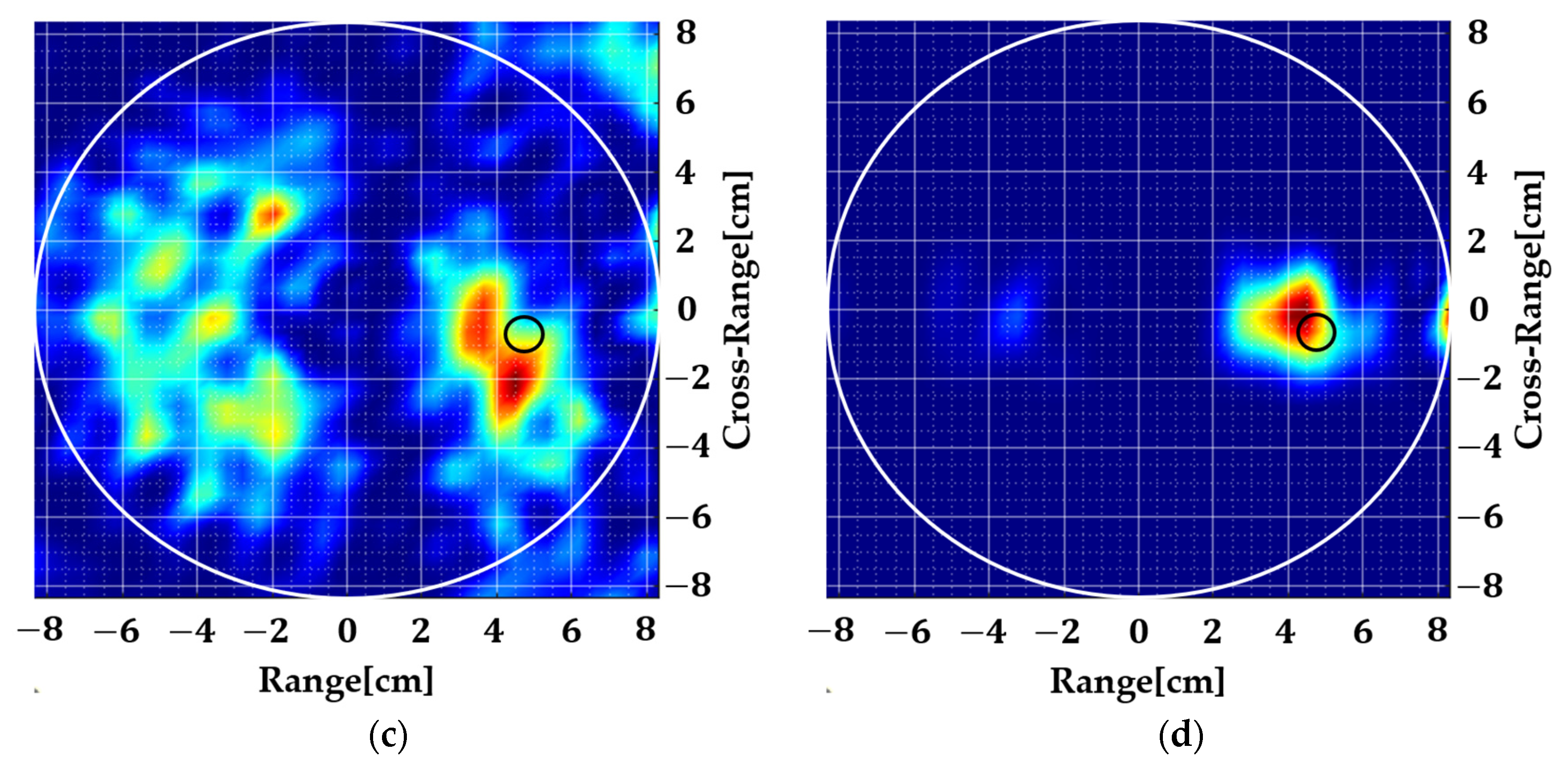
4. Measured Results
4.1. Homogeneous Background
4.2. Inhomogeneous Background
5. Conclusions
Author Contributions
Funding
Institutional Review Board Statement
Informed Consent Statement
Data Availability Statement
Conflicts of Interest
References
- Pang, L.; Liu, H.; Chen, Y.; Miao, J. Real-time concealed object detection from passive millimeter wave images based on the YOLOv3 algorithm. Sensors 2020, 20, 1678. [Google Scholar] [CrossRef] [PubMed] [Green Version]
- Islam, M.T.; Mahmud, M.Z.; Islam, M.T.; Kibria, S.; Samsuzzaman, M. A low cost and portable microwave imaging system for breast tumor detection using UWB directional antenna array. Sci. Rep. 2019, 9, 15491. [Google Scholar] [CrossRef] [PubMed] [Green Version]
- Li, Z.; Jin, T.; Dai, Y.; Song, Y. Through-Wall Multi-Subject Localization and Vital Signs Monitoring Using UWB MIMO Imaging Radar. Remote Sens. 2021, 13, 2905. [Google Scholar] [CrossRef]
- Sobkiewicz, P.; Bieńkowski, P.; Błażejewski, W. Microwave Non-Destructive Testing for Delamination Detection in Layered Composite Pipelines. Sensors 2021, 21, 4168. [Google Scholar] [CrossRef] [PubMed]
- Shao, W.; McCollough, T. Advances in microwave near-field imaging: Prototypes, systems, and applications. IEEE Microw. Mag. 2020, 21, 94–119. [Google Scholar] [CrossRef] [PubMed]
- Mustafa, S.; Mohammed, B.; Abbosh, A. Novel preprocessing techniques for accurate microwave imaging of human brain. IEEE Antennas Wirel. Propag. Lett. 2013, 12, 460–463. [Google Scholar] [CrossRef]
- Mustafa, S. Wavelet-matched filters at microwave frequencies for stroke diagnosis. IEEE Trans. Antennas Propag. 2018, 66, 6273–6282. [Google Scholar] [CrossRef]
- Mehranpour, M.; Jarchi, S.; Keshtkar, A.; Ghorbani, A.; Araghi, A.; Yurduseven, O.; Khalily, M. Robust breast cancer imaging based on a hybrid artifact suppression method for early-stage tumor detection. IEEE Access 2020, 8, 206790–206805. [Google Scholar] [CrossRef]
- Ghimire, J.; Diba, F.D.; Kim, J.-H.; Choi, D.-Y. Vivaldi antenna arrays feed by frequency-independent phase Shifter for high directivity and gain used in microwave sensing and communication applications. Sensors 2021, 21, 6091. [Google Scholar] [CrossRef]
- Shao, W.; Edalati, A.; McCollough, T.R.; McCollough, W.J. A time-domain measurement system for UWB microwave imaging. IEEE Trans. Microw. Theory Tech. 2018, 66, 2265–2275. [Google Scholar] [CrossRef]
- Alqadami, A.S.; Trakic, A.; Stancombe, A.E.; Mohammed, B.; Bialkowski, K.; Abbosh, A. Flexible electromagnetic cap for head imaging. IEEE Trans. Biomed. Circuits Syst. 2020, 14, 1097–1107. [Google Scholar] [CrossRef] [PubMed]
- Fedeli, A.; Estatico, C.; Pastorino, M.; Randazzo, A. Microwave detection of brain injuries by means of a hybrid imaging method. IEEE Open J. Antennas Propag. 2020, 1, 513–523. [Google Scholar] [CrossRef]
- Yoon, S.-W.; Kim, S.-B.; Jung, J.-H.; Cha, S.-B.; Baek, Y.-S.; Koo, B.-T.; Choi, I.-O.; Park, S.-H. Efficient Classification of Birds and Drones Considering Real Observation Scenarios Using FMCW Radar. J. Electromagn. Eng. Sci. 2021, 21, 270–281. [Google Scholar] [CrossRef]
- Nam, J.-H.; Rim, J.-W.; Lee, H.; Koh, I.-S.; Song, J.-H. Modeling of monopulse radar signals reflected from ground clutter in a time domain considering doppler effects. J. Electromagn. Eng. Sci. 2020, 20, 190–198. [Google Scholar] [CrossRef]
- Guo, G.; Guo, L.-X.; Wang, R.; Li, L. An ISAR Imaging Framework for Large and Complex Targets Using TDSBR. IEEE Antennas Wirel. Propag. Lett. 2021, 20, 1928–1932. [Google Scholar] [CrossRef]
- Guo, G.; Guo, L.-X.; Wang, R. ISAR image algorithm using time-domain scattering echo simulated by TDPO method. IEEE Antennas Wirel. Propag. Lett. 2020, 19, 1331–1335. [Google Scholar] [CrossRef]
- Shao, W.; Edalati, A.; McCollough, T.R.; McCollough, W.J. A phase confocal method for near-field microwave imaging. IEEE Trans. Microw. Theory Tech. 2017, 65, 2508–2515. [Google Scholar] [CrossRef]
- Shao, W.; McCollough, T.R.; McCollough, W.J. A phase shift and sum method for UWB radar imaging in dispersive media. IEEE Trans. Microw. Theory Tech. 2019, 67, 2018–2027. [Google Scholar] [CrossRef]
- Kotaru, M.; Joshi, K.; Bharadia, D.; Katti, S. Spotfi: Decimeter level localization using wifi. In Proceedings of the 2015 ACM Conference on Special Interest Group on Data Communication, New York, NY, USA, 17–21 August 2015. [Google Scholar]
- Owda, A.Y.; Owda, M.; Rezgui, N.D. Synthetic aperture radar imaging for burn wounds diagnostics. Sensors 2020, 20, 847. [Google Scholar] [CrossRef] [Green Version]
- Ozdemir, C. Inverse Synthetic Aperture Radar Imaging with MATLAB Algorithms; John Wiley & Sons: Hoboken, NJ, USA, 2012; Volume 210. [Google Scholar]
- Trakic, A.; Brankovic, A.; Zamani, A.; Nguyen-Trong, N.; Mohammed, B.; Stancombe, A.; Guo, L.; Bialkowski, K.; Abbosh, A. Expedited stroke imaging with electromagnetic polar sensitivity encoding. IEEE Trans. Antennas Propag. 2020, 68, 8072–8081. [Google Scholar] [CrossRef]
- Chen, Y.-J.; Zhang, Q.; Luo, Y.; Li, K.-M. Multi-Target Radar Imaging Based on Phased-MIMO Technique—Part I: Imaging Algorithm. IEEE Sens. J. 2017, 17, 6185–6197. [Google Scholar] [CrossRef]
- Li, S.; Sun, H.; Zhu, B.; Liu, R. Two-dimensional NUFFT-based algorithm for fast near-field imaging. IEEE Antennas Wirel. Propag. Lett. 2010, 9, 814–817. [Google Scholar] [CrossRef]
- Cheng, W.; Zhang, Z.; Cao, H.; He, Z.; Zhu, G. A comparative study of information-based source number estimation methods and experimental validations on mechanical systems. Sensors 2014, 14, 7625–7646. [Google Scholar] [CrossRef] [Green Version]
- Tournier, P.H.; Bonazzoli, M.; Dolean, V.; Rapetti, F.; Hecht, F.; Nataf, F.; Aliferis, I.; El Kanfoud, I.; Migliaccio, C.; De Buhan, M.; et al. Numerical Modeling and High-Speed Parallel Computing: New Perspectives on Tomographic Microwave Imaging for Brain Stroke Detection and Monitoring. IEEE Antennas Propag. Mag. 2017, 59, 98–110. [Google Scholar] [CrossRef] [Green Version]


| Reference | Antenna Configuration/Locations | Method | Bandwidth | Anomaly Diameter (mm) |
|---|---|---|---|---|
| [6] | Monostatic (16 and 32 antennas) | TD | 1–4 GHz | 28 × 14 |
| [7] (Simulated) | Monostatic (14 antennas) | TD | 1.5 and 2 GHz | 7.2 × 6.3 × 3.6 |
| [8] | Multistatic (37 antennas) | TD | 2.2–13.5 GHz | 5 |
| [18] | Multistatic (2 antennas; 19 × 24 locations) | FD | 2–7 GHz | 19.5 and 17 × 10 × 12 |
| [26] | Multistatic (160 Antennas) | Quantitative Imaging | 0.9–1.8 GHz | 39 × 23 × 23 |
| This Work | Monostatic (24 locations) | FD | 1–8.5 GHz | 10 |
Publisher’s Note: MDPI stays neutral with regard to jurisdictional claims in published maps and institutional affiliations. |
© 2022 by the authors. Licensee MDPI, Basel, Switzerland. This article is an open access article distributed under the terms and conditions of the Creative Commons Attribution (CC BY) license (https://creativecommons.org/licenses/by/4.0/).
Share and Cite
Bilal, A.; Cho, C.S. Localization of Dielectric Anomalies with Multi-Monostatic S11 Using 2D MUSIC Algorithm with Spatial Smoothing. Sensors 2022, 22, 5293. https://doi.org/10.3390/s22145293
Bilal A, Cho CS. Localization of Dielectric Anomalies with Multi-Monostatic S11 Using 2D MUSIC Algorithm with Spatial Smoothing. Sensors. 2022; 22(14):5293. https://doi.org/10.3390/s22145293
Chicago/Turabian StyleBilal, Ahmad, and Choon Sik Cho. 2022. "Localization of Dielectric Anomalies with Multi-Monostatic S11 Using 2D MUSIC Algorithm with Spatial Smoothing" Sensors 22, no. 14: 5293. https://doi.org/10.3390/s22145293
APA StyleBilal, A., & Cho, C. S. (2022). Localization of Dielectric Anomalies with Multi-Monostatic S11 Using 2D MUSIC Algorithm with Spatial Smoothing. Sensors, 22(14), 5293. https://doi.org/10.3390/s22145293