
Optimal LiDAR Data Resolution Analysis for Object Classification


Abstract
:1. Introduction
2. Methods
2.1. Lidar Data Collection and Trade-Offs
2.2. Input Data Sets and Resolution
2.2.1. Sydney Urban Data Set
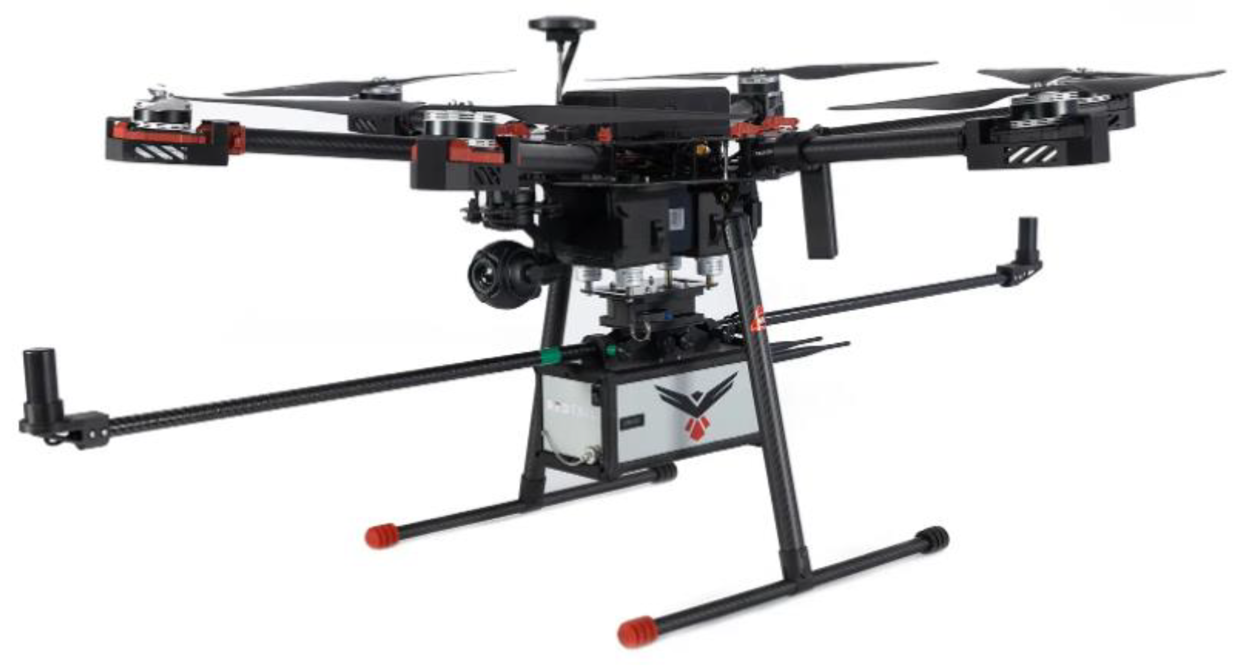
2.2.2. RedTail LiDAR System Data Set
2.3. Data Analysis
2.3.1. Detection of Objects within a Larger Set
2.3.2. Classification of Objects
3. Results
3.1. Results for Sydney Urban Data Set
3.2. Results for RedTail RTL-450 Data Set
4. Discussion
5. Conclusions
Author Contributions
Funding
Institutional Review Board Statement
Informed Consent Statement
Data Availability Statement
Acknowledgments
Conflicts of Interest
References
- Xu, X.; Corrigan, D.; Dehghani, A.; Caulfield, S.; Moloney, D. 3D object recognition based on volumetric representation using convolutional neural networks. In International Conference on Articulated Motion and Deformable Objects; Springer: Cham, Switzerland, 2016; pp. 147–156. [Google Scholar]
- Verschoof-van der Vaart, W.B.; Lambers, K. Learning to look at LiDAR: The use of R-CNN in the automated detection of archaeological objects in LiDAR data from the Netherlands. J. Comput. Appl. Archaeol. 2019, 2, 31–40. [Google Scholar] [CrossRef] [Green Version]
- Prokhorov, D. A convolutional learning system for object classification in 3-D LIDAR data. IEEE Trans. Neural Netw. 2010, 21, 858–863. [Google Scholar] [CrossRef] [PubMed]
- Qi, C.R.; Su, H.; Mo, K.; Guibas, L.J. PointNet: Deep learning on point sets for 3D classification and segmentation. In Proceedings of the IEEE Conference on Computer Vision and Pattern Recognition (CVPR), Honolulu, HI, USA, 21–26 July 2017; pp. 77–85. [Google Scholar]
- Kowalczuk, Z.; Szymański, K. Classification of objects in the LIDAR point clouds using Deep Neural Networks based on the PointNet model. IFAC-PapersOnLine 2019, 52, 416–421. [Google Scholar] [CrossRef]
- Wang, Y.; Sun, Y.; Liu, Z.; Sarma, S.E.; Bronstein, M.M.; Solomon, J. Dynamic graph CNN for learning on point clouds. ACM Trans. Graph. 2019, 38, 146. [Google Scholar] [CrossRef] [Green Version]
- He, X.; Wang, A.; Ghamisi, P.; Li, G.; Chen, Y. LiDAR data classification using spatial transformation and CNN. IEEE Geosci. Remote Sens. Lett. 2018, 16, 125–129. [Google Scholar] [CrossRef]
- Jaderberg, M.; Simonyan, K.; Zisserman, A.; Kavukcuoglu, K. Spatial transformer networks. In Proceedings of the 28th International Conference on Neural Information Processing Systems, Cambridge, MA, USA, 7–12 December 2015; Volume 25, pp. 2017–2025. [Google Scholar]
- Maturana, D.; Scherer, S. Voxnet: A 3d convolutional neural network for real-time object recognition. In Proceedings of the 2015 IEEE/RSJ International Conference on Intelligent Robots and Systems (IROS) 2015, Hamburg, Germany, 17 December 2015; pp. 922–928. [Google Scholar]
- Hackel, T.; Savinov, N.; Ladicky, L.; Wegner, J.D.; Schindler, K.; Pollefeys, M. Semantic3d.net: A new large-scale point cloud classification benchmark. arXiv 2017, arXiv:1704.03847. [Google Scholar] [CrossRef] [Green Version]
- Liu, X.; Zhang, Z.; Peterson, J.; Chandra, S. The effect of LiDAR data density on DEM accuracy. In Proceedings of the International Congress on Modelling and Simulation (MODSIM07): Modelling and Simulation Society of Australia and New Zealand Inc., Christchurch, New Zealand, 10–13 December 2007; pp. 1363–1369. [Google Scholar]
- Peng, X.; Zhao, A.; Chen, Y.; Chen, Q.; Liu, H. Tree height measurements in degraded tropical forests based on UAV-LiDAR data of different point cloud densities: A case study on Dacrydium pierrei in China. Forests 2021, 12, 328. [Google Scholar] [CrossRef]
- Błaszczak-Bąk, W.; Janicka, J.; Suchocki, C.; Masiero, A.; Sobieraj-Żłobińska, A. Down-sampling of large LiDAR dataset in the context of off-road objects extraction. Geosciences 2020, 10, 219. [Google Scholar] [CrossRef]
- Tomljenovic, I.; Rousell, A. Influence of point cloud density on the results of automated Object-Based building extraction from ALS data. In Proceedings of the AGILE’2014 International Conference on Geographic Information Science, Castellón, Spain, 3–6 June 2014; ISBN 978-90-816960-4-3. [Google Scholar]
- Cloud Compare (Version 2.6.1) User Manual. Available online: https://www.cloudcompare.org/doc/qCC/CloudCompare%20v2.6.1%20-%20User%20manual.pdf (accessed on 1 May 2022).
- RedTail Application Sheet—Construction. Available online: https://cdn.sanity.io/files/06v39dn4/production/51cf4ad94abef43f30e875bd330ea2d767e8781c.pdf (accessed on 1 May 2022).
- Börcs, A.; Nagy, B.; Benedek, C. Fast 3-D urban object detection on streaming point clouds. In Proceedings of the European Conference on Computer Vision, Zurich, Switzerland, 6–12 September 2014; Springer: Cham, Switzerland, 2014; pp. 628–639. [Google Scholar] [CrossRef] [Green Version]


| Altitude (m) | Flight Speed (m/s) | ||||||||
|---|---|---|---|---|---|---|---|---|---|
| 4 | 6 | 8 | 10 | 12 | 14 | 16 | 18 | 20 | |
| 40 | 1717 | 1145 | 859 | 687 | 572 | 491 | 429 | 382 | 343 |
| 60 | 1145 | 763 | 572 | 458 | 382 | 327 | 286 | 254 | 229 |
| 80 | 859 | 572 | 429 | 343 | 286 | 245 | 215 | 191 | 172 |
| 100 | 687 | 458 | 343 | 275 | 229 | 196 | 172 | 153 | 137 |
| 120 | 572 | 382 | 286 | 229 | 191 | 164 | 143 | 127 | 114 |
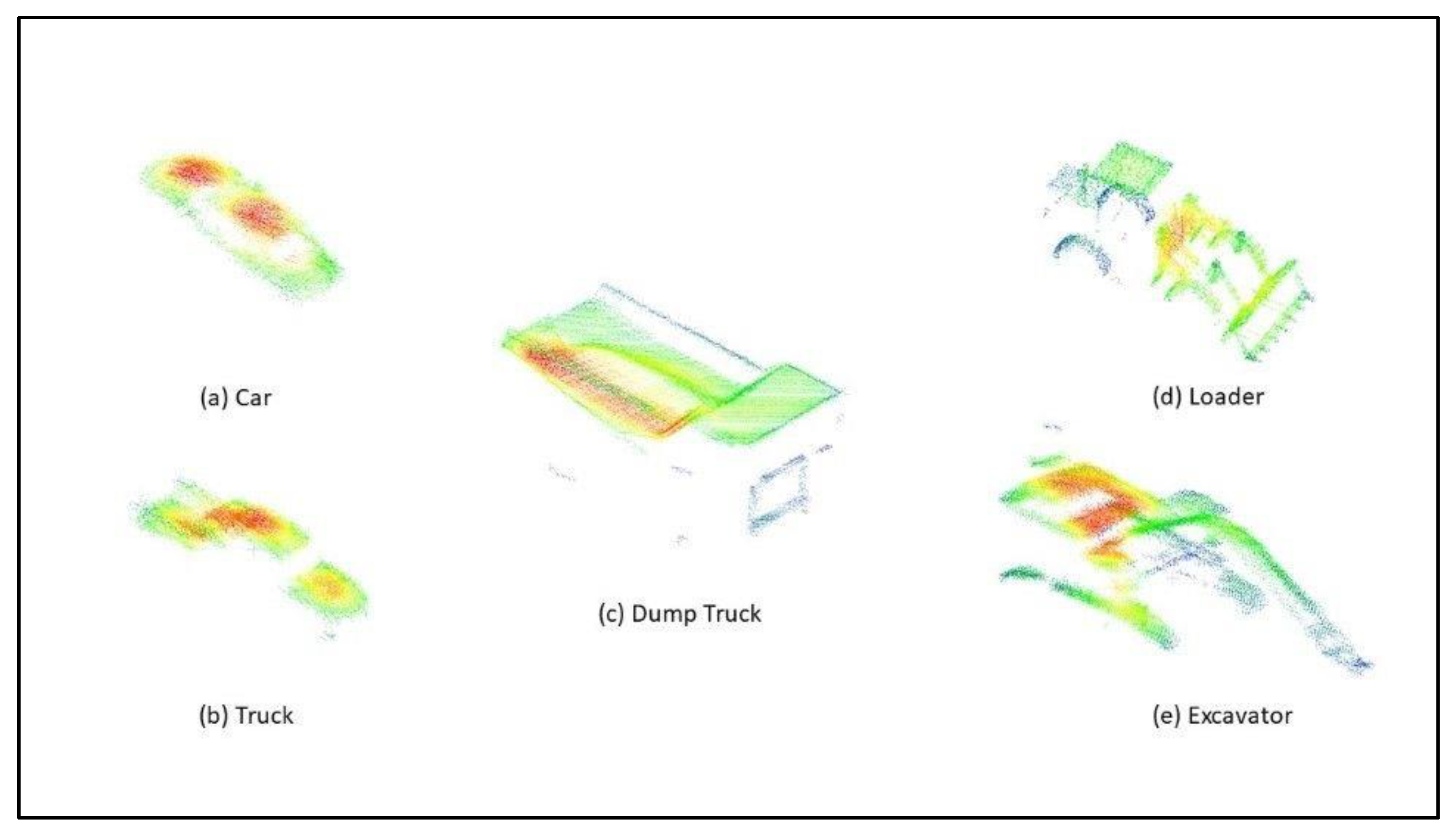
| Car | Trucks | Dump Trucks | Loaders | Excavators | |
|---|---|---|---|---|---|
| Representative Surface Density (points/m2) | 762.5 | 787.2 | 705.0 | 761.8 | 722.8 |
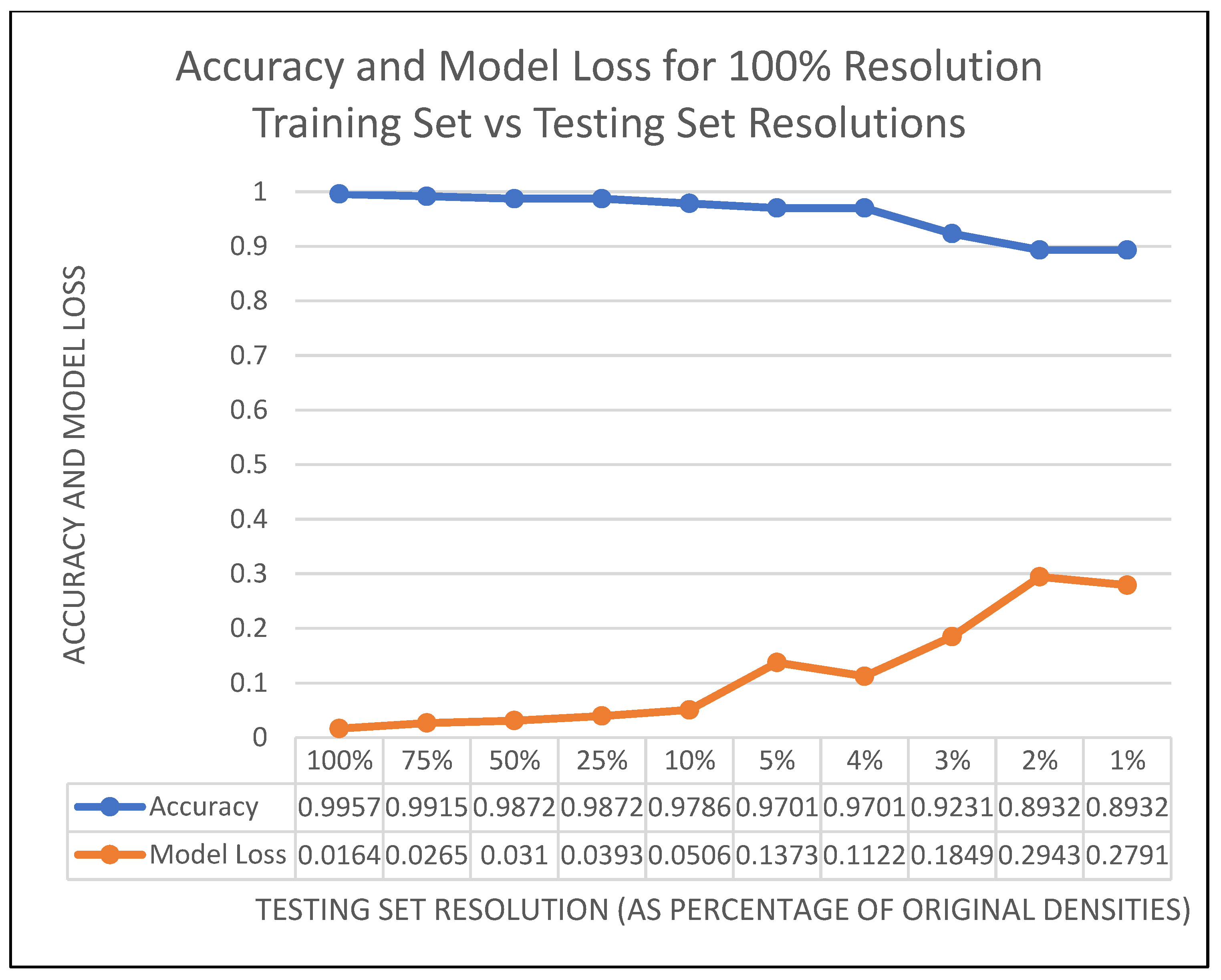
| Data Resolution | 100% | 75% | 50% | 25% |
|---|---|---|---|---|
| Accuracy | 0.6718 | 0.3029 | 0.2413 | 0.1753 |
Publisher’s Note: MDPI stays neutral with regard to jurisdictional claims in published maps and institutional affiliations. |
© 2022 by the authors. Licensee MDPI, Basel, Switzerland. This article is an open access article distributed under the terms and conditions of the Creative Commons Attribution (CC BY) license (https://creativecommons.org/licenses/by/4.0/).
Share and Cite
Darrah, M.; Richardson, M.; DeRoos, B.; Wathen, M. Optimal LiDAR Data Resolution Analysis for Object Classification. Sensors 2022, 22, 5152. https://doi.org/10.3390/s22145152
Darrah M, Richardson M, DeRoos B, Wathen M. Optimal LiDAR Data Resolution Analysis for Object Classification. Sensors. 2022; 22(14):5152. https://doi.org/10.3390/s22145152
Chicago/Turabian StyleDarrah, Marjorie, Matthew Richardson, Bradley DeRoos, and Mitchell Wathen. 2022. "Optimal LiDAR Data Resolution Analysis for Object Classification" Sensors 22, no. 14: 5152. https://doi.org/10.3390/s22145152
APA StyleDarrah, M., Richardson, M., DeRoos, B., & Wathen, M. (2022). Optimal LiDAR Data Resolution Analysis for Object Classification. Sensors, 22(14), 5152. https://doi.org/10.3390/s22145152