
Semi-ProtoPNet Deep Neural Network for the Classification of Defective Power Grid Distribution Structures


Abstract
:1. Introduction
- The first contribution is due to the need for a small database to train the proposed Semi-ProtoPNet. Typically, deep neural networks need a large database to train the model. From the proposed method, high accuracy was obtained using a small dataset, which would enable the use of this model for field applications.
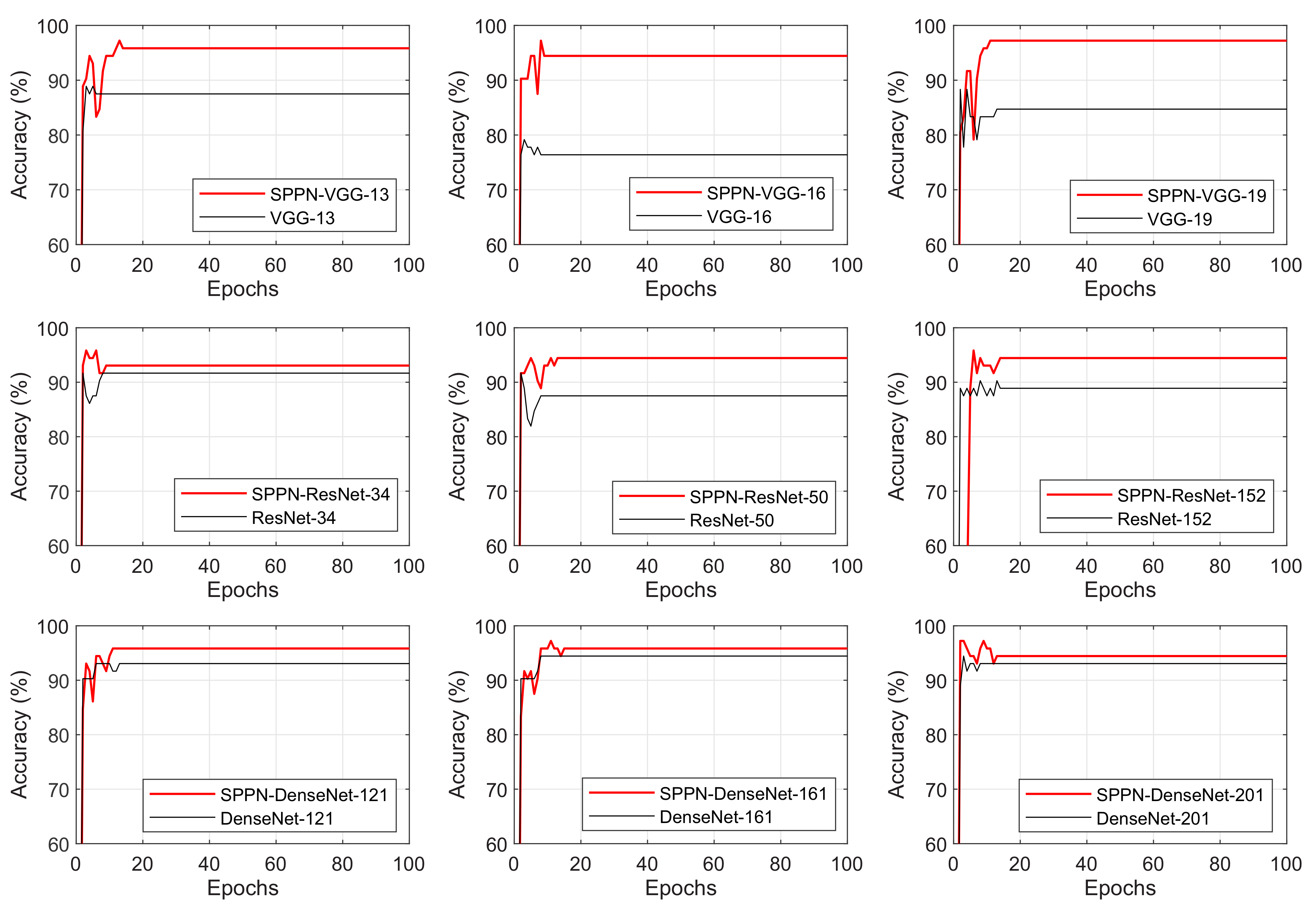
- The proposed model has better accuracy than the state-of-the-art models (VGG-13, VGG-16, VGG-19, ResNet-34, ResNet-50, ResNet-152, DenseNet-121, DenseNet-161, DenseNet-201, ProtoPNet, NP-ProtoPNet, Gen-ProtoPNet, and Ps-ProtoPNet) for image classification. This is because the Semi-ProtoPNet uses a generalized convolutional layer that helps it to use both positive and negative reasoning processes. The idea of using a negative reasoning process is similar to the idea of solving a multiple-choice question, where it becomes helpful to rule out the options that are surely not an answer to the question.
- The third contribution is related to the use of real inspection images of the electrical power grid. There is great difficulty in obtaining an adequate database to classify the conditions of distribution networks. This occurs because the failures are difficult to find due to the large extension of the network, among other reasons. In this paper, the analysis of adverse conditions is performed based on real inspection images of problematic branches reported by the electric utility.
- Considering that the proposed model does not focus on a specific condition or component, it has the ability to handle large variations between inspection photos with different image frames, brightness, and backgrounds. This makes inspection easier for the operator, as it is easier to take the photos; therefore, it is a more comprehensive method for this evaluation.
2. Related Works and Considered Dataset
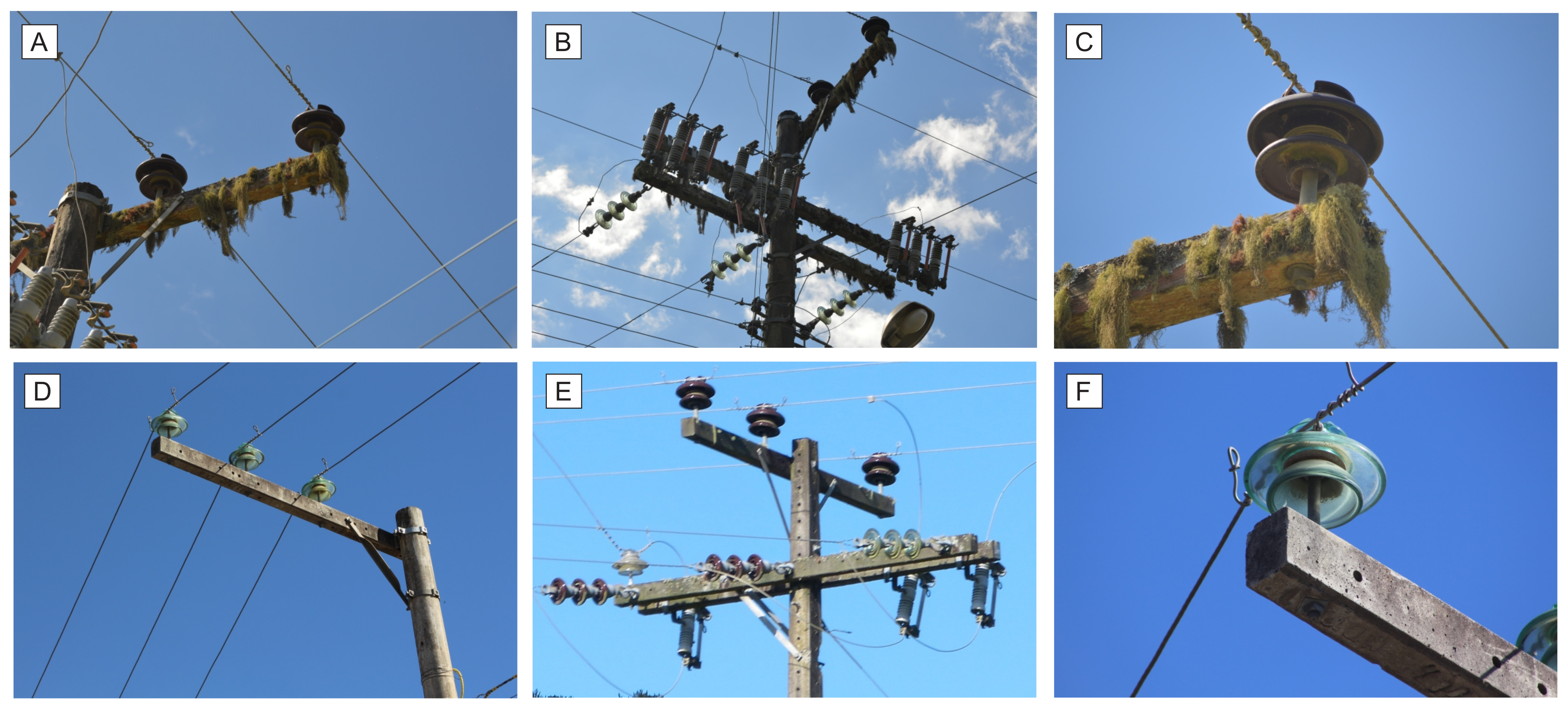
Dataset
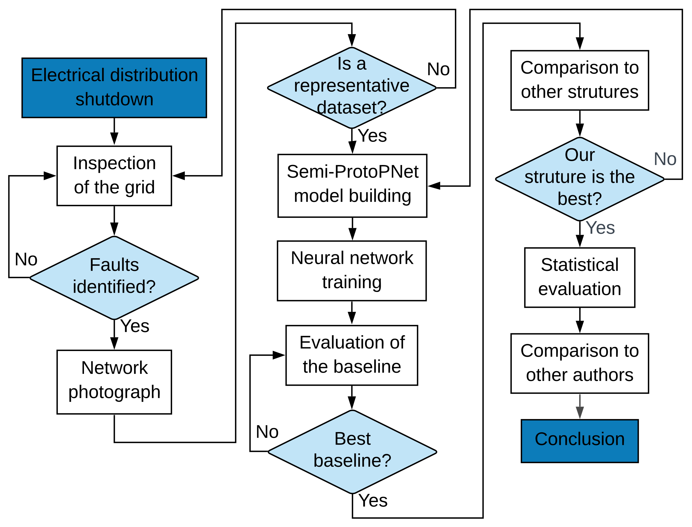
3. Methodology
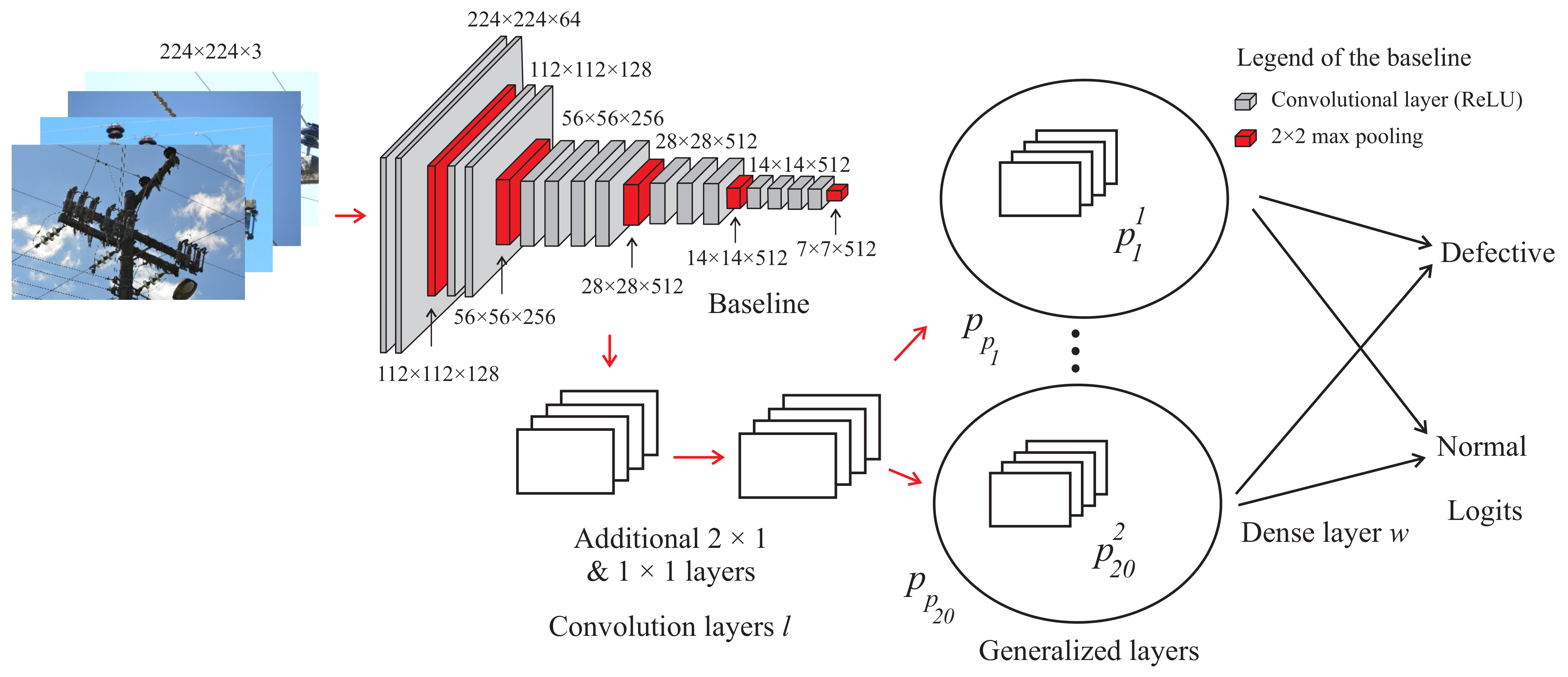
3.1. Architecture
Training Procedure
- The proposed method does not replace prototypes with the latent patches of the training images; these prototypes have values very close to the pixel values of the training images.
- The prototypes with spatial dimensions bigger than are used. With the generalized distance function d, it is possible to use prototypes with any type of spatial dimensions—that is, square spatial dimensions as well as rectangular spatial dimensions.
- The Semi-ProtoPNet does not perform convex optimization of the last layer to maintain the impact of the negative reasoning process on the image classification, whereas the ProtoPNet model emphasizes the positive reasoning process. Further, the nonoptimization of the last layer reduces the training time considerably.
- Using the Semi-ProtoPNet, regardless of the weight given to the positive class, it gives exactly equal to the negative of that weight to the negative class, and this weight is not reduced to zero, unlike ProtoPNet. By doing so, we equally consider both positive reasoning and negative reasoning to classify the images.
3.2. Limitations
3.3. Performance Evaluation Metrics
4. Results and Discussion
4.1. Dataset Evaluation
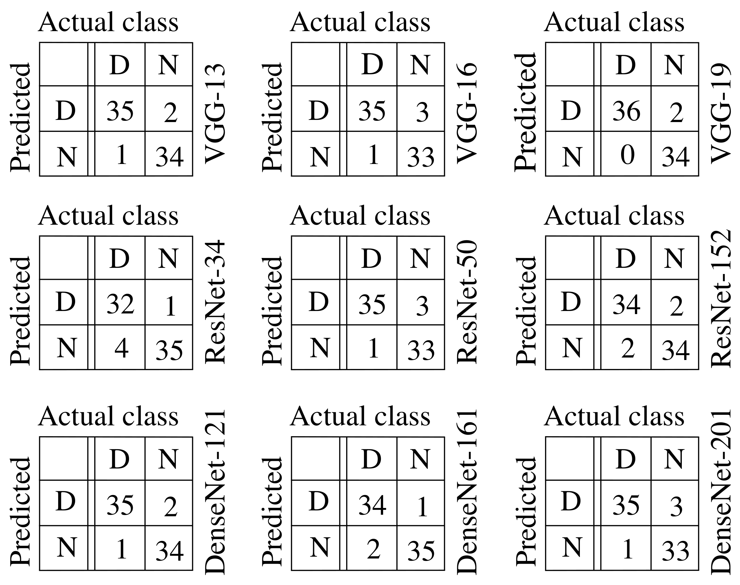
4.2. Confusion Matrices
4.3. Baseline Evaluation
4.4. Benchmarking
4.4.1. Test of Hypothesis for the Accuracy and Statistical Evaluation
4.4.2. State-of-the-Art Approaches
5. Conclusions
Author Contributions
Funding
Informed Consent Statement
Data Availability Statement
Conflicts of Interest
References
- Ma, D.; Jin, L.; He, J.; Gao, K. Classification of partial discharge severities of ceramic insulators based on texture analysis of UV pulses. High Volt. 2021, 6, 986–996. [Google Scholar] [CrossRef]
- Stefenon, S.F.; Freire, R.Z.; Meyer, L.H.; Corso, M.P.; Sartori, A.; Nied, A.; Klaar, A.C.R.; Yow, K.C. Fault detection in insulators based on ultrasonic signal processing using a hybrid deep learning technique. IET Sci. Meas. Technol. 2020, 14, 953–961. [Google Scholar] [CrossRef]
- Ramesh, M.; Cui, L.; Shtessel, Y.; Gorur, R. Failure studies of polymeric insulating materials using sliding mode observer. Int. J. Electr. Power Energy Syst. 2021, 126, 106539. [Google Scholar] [CrossRef]
- Sopelsa Neto, N.F.; Stefenon, S.F.; Meyer, L.H.; Bruns, R.; Nied, A.; Seman, L.O.; Gonzalez, G.V.; Leithardt, V.R.Q.; Yow, K.C. A Study of Multilayer Perceptron Networks Applied to Classification of Ceramic Insulators Using Ultrasound. Appl. Sci. 2021, 11, 1592. [Google Scholar] [CrossRef]
- Castillo-Sierra, R.; Oviedo-Trespalacios, O.; Candelo-Becerra, J.E.; Soto, J.D.; Calle, M. A novel method for prediction of washing cycles of electrical insulators in high pollution environments. Int. J. Electr. Power Energy Syst. 2021, 130, 107026. [Google Scholar] [CrossRef]
- Han, J.; Yang, Z.; Xu, H.; Hu, G.; Zhang, C.; Li, H.; Lai, S.; Zeng, H. Search Like an Eagle: A Cascaded Model for Insulator Missing Faults Detection in Aerial Images. Energies 2020, 13, 713. [Google Scholar] [CrossRef] [Green Version]
- Polisetty, S.; El-Hag, A.; Jayram, S. Classification of common discharges in outdoor insulation using acoustic signals and artificial neural network. High Volt. 2019, 4, 333–338. [Google Scholar] [CrossRef]
- Yang, L.; Fan, J.; Liu, Y.; Li, E.; Peng, J.; Liang, Z. A Review on State-of-the-Art Power Line Inspection Techniques. IEEE Trans. Instrum. Meas. 2020, 69, 9350–9365. [Google Scholar] [CrossRef]
- Stefenon, S.F.; Bruns, R.; Sartori, A.; Meyer, L.H.; Ovejero, R.G.; Leithardt, V.R.Q. Analysis of the Ultrasonic Signal in Polymeric Contaminated Insulators Through Ensemble Learning Methods. IEEE Access 2022, 10, 33980–33991. [Google Scholar] [CrossRef]
- Rocha, P.; Costa, E.; Serres, A.; Xavier, G.; Peixoto, J.; Lins, R. Inspection in overhead insulators through the analysis of the irradiated RF spectrum. Int. J. Electr. Power Energy Syst. 2019, 113, 355–361. [Google Scholar] [CrossRef]
- Lin, Y.; Yin, F.; Liu, Y.; Wang, L.; Wu, K. Influence of vulcanization factors on UV-A resistance of silicone rubber for outdoor insulators. IEEE Trans. Dielectr. Electr. Insul. 2020, 27, 296–304. [Google Scholar] [CrossRef]
- Jin, L.; Ai, J.; Tian, Z.; Zhang, Y. Detection of polluted insulators using the information fusion of multispectral images. IEEE Trans. Dielectr. Electr. Insul. 2017, 24, 3530–3538. [Google Scholar] [CrossRef]
- Nguyen, V.N.; Jenssen, R.; Roverso, D. Automatic autonomous vision-based power line inspection: A review of current status and the potential role of deep learning. Int. J. Electr. Power Energy Syst. 2018, 99, 107–120. [Google Scholar] [CrossRef] [Green Version]
- Chen, C.; Li, O.; Tao, C.; Barnett, A.J.; Su, J.; Rudin, C. This looks like that: Deep learning for interpretable image recognition. arXiv 2018, arXiv:1806.10574. [Google Scholar]
- Singh, G.; Yow, K.C. These do not Look Like Those: An Interpretable Deep Learning Model for Image Recognition. IEEE Access 2021, 9, 41482–41493. [Google Scholar] [CrossRef]
- Singh, G.; Yow, K.C. An Interpretable Deep Learning Model for Covid-19 Detection With Chest X-Ray Images. IEEE Access 2021, 9, 85198–85208. [Google Scholar] [CrossRef]
- Singh, G.; Yow, K.C. Object or Background: An Interpretable Deep Learning Model for COVID-19 Detection from CT-Scan Images. Diagnostics 2021, 11, 1732. [Google Scholar] [CrossRef]
- Singh, G. Think positive: An interpretable neural network for image recognition. Neural Netw. 2022, 151, 178–189. [Google Scholar] [CrossRef]
- Medeiros, A.; Sartori, A.; Stefenon, S.F.; Meyer, L.H.; Nied, A. Comparison of artificial intelligence techniques to failure prediction in contaminated insulators based on leakage current. J. Intell. Fuzzy Syst. 2021, 42, 3285–3298. [Google Scholar] [CrossRef]
- Corso, M.P.; Perez, F.L.; Stefenon, S.F.; Yow, K.C.; García Ovejero, R.; Leithardt, V.R.Q. Classification of Contaminated Insulators Using k-Nearest Neighbors Based on Computer Vision. Computers 2021, 10, 112. [Google Scholar] [CrossRef]
- Cao, B.; Wang, L.; Yin, F. A Low-Cost Evaluation and Correction Method for the Soluble Salt Components of the Insulator Contamination Layer. IEEE Sens. J. 2019, 19, 5266–5273. [Google Scholar] [CrossRef]
- Stefenon, S.F.; Seman, L.O.; Sopelsa Neto, N.F.; Meyer, L.H.; Nied, A.; Yow, K.C. Echo state network applied for classification of medium voltage insulators. Int. J. Electr. Power Energy Syst. 2022, 134, 107336. [Google Scholar] [CrossRef]
- Stefenon, S.F.; Seman, L.O.; Pavan, B.A.; Ovejero, R.G.; Leithardt, V.R.Q. Optimal design of electrical power distribution grid spacers using finite element method. IET Gener. Transm. Distrib. 2022, 16, 1865–1876. [Google Scholar] [CrossRef]
- Manninen, H.; Ramlal, C.J.; Singh, A.; Rocke, S.; Kilter, J.; Landsberg, M. Toward automatic condition assessment of high-voltage transmission infrastructure using deep learning techniques. Int. J. Electr. Power Energy Syst. 2021, 128, 106726. [Google Scholar] [CrossRef]
- Alhassan, A.B.; Zhang, X.; Shen, H.; Xu, H. Power transmission line inspection robots: A review, trends and challenges for future research. Int. J. Electr. Power Energy Syst. 2020, 118, 105862. [Google Scholar] [CrossRef]
- Ibrahim, A.; Dalbah, A.; Abualsaud, A.; Tariq, U.; El-Hag, A. Application of Machine Learning to Evaluate Insulator Surface Erosion. IEEE Trans. Instrum. Meas. 2020, 69, 314–316. [Google Scholar] [CrossRef]
- Prates, R.M.; Cruz, R.; Marotta, A.P.; Ramos, R.P.; Simas Filho, E.F.; Cardoso, J.S. Insulator visual non-conformity detection in overhead power distribution lines using deep learning. Comput. Electr. Eng. 2019, 78, 343–355. [Google Scholar] [CrossRef]
- Hagmar, H.; Tong, L.; Eriksson, R.; Tuan, L.A. Voltage Instability Prediction Using a Deep Recurrent Neural Network. IEEE Trans. Power Syst. 2021, 36, 17–27. [Google Scholar] [CrossRef]
- Sun, J.; Zhang, H.; Li, Q.; Liu, H.; Lu, X.; Hou, K. Contamination degree prediction of insulator surface based on exploratory factor analysis-least square support vector machine combined model. High Volt. 2021, 6, 264–277. [Google Scholar] [CrossRef]
- Pernebayeva, D.; Irmanova, A.; Sadykova, D.; Bagheri, M.; James, A. High voltage outdoor insulator surface condition evaluation using aerial insulator images. High Volt. 2019, 4, 178–185. [Google Scholar] [CrossRef]
- Sampedro, C.; Rodriguez-Vazquez, J.; Rodriguez-Ramos, A.; Carrio, A.; Campoy, P. Deep Learning-Based System for Automatic Recognition and Diagnosis of Electrical Insulator Strings. IEEE Access 2019, 7, 101283–101308. [Google Scholar] [CrossRef]
- Tao, X.; Zhang, D.; Wang, Z.; Liu, X.; Zhang, H.; Xu, D. Detection of Power Line Insulator Defects Using Aerial Images Analyzed With Convolutional Neural Networks. IEEE Trans. Syst. Man. Cybern. Syst. 2020, 50, 1486–1498. [Google Scholar] [CrossRef]
- Han, J.; Yang, Z.; Zhang, Q.; Chen, C.; Li, H.; Lai, S.; Hu, G.; Xu, C.; Xu, H.; Wang, D.; et al. A Method of Insulator Faults Detection in Aerial Images for High-Voltage Transmission Lines Inspection. Appl. Sci. 2019, 9, 2009. [Google Scholar] [CrossRef] [Green Version]
- Miao, X.; Liu, X.; Chen, J.; Zhuang, S.; Fan, J.; Jiang, H. Insulator Detection in Aerial Images for Transmission Line Inspection Using Single Shot Multibox Detector. IEEE Access 2019, 7, 9945–9956. [Google Scholar] [CrossRef]
- Li, X.; Su, H.; Liu, G. Insulator Defect Recognition Based on Global Detection and Local Segmentation. IEEE Access 2020, 8, 59934–59946. [Google Scholar] [CrossRef]
- Li, F.; Xin, J.; Chen, T.; Xin, L.; Wei, Z.; Li, Y.; Zhang, Y.; Jin, H.; Tu, Y.; Zhou, X.; et al. An Automatic Detection Method of Bird’s Nest on Transmission Line Tower Based on Faster-RCNN. IEEE Access 2020, 8, 164214–164221. [Google Scholar] [CrossRef]
- Liu, C.; Wu, Y.; Liu, J.; Sun, Z. Improved YOLOv3 Network for Insulator Detection in Aerial Images with Diverse Background Interference. Electronics 2021, 10, 771. [Google Scholar] [CrossRef]
- Liu, Y.; Ji, X.; Pei, S.; Ma, Z.; Zhang, G.; Lin, Y.; Chen, Y. Research on automatic location and recognition of insulators in substation based on YOLOv3. High Volt. 2020, 5, 62–68. [Google Scholar] [CrossRef]
- Teimourzadeh, H.; Moradzadeh, A.; Shoaran, M.; Mohammadi-Ivatloo, B.; Razzaghi, R. High Impedance Single-Phase Faults Diagnosis in Transmission Lines via Deep Reinforcement Learning of Transfer Functions. IEEE Access 2021, 9, 15796–15809. [Google Scholar] [CrossRef]
- Fahim, S.R.; Sarker, S.K.; Muyeen, S.; Das, S.K.; Kamwa, I. A deep learning based intelligent approach in detection and classification of transmission line faults. Int. J. Electr. Power Energy Syst. 2021, 133, 107102. [Google Scholar] [CrossRef]
- Zhao, M.; Zhong, S.; Fu, X.; Tang, B.; Dong, S.; Pecht, M. Deep Residual Networks With Adaptively Parametric Rectifier Linear Units for Fault Diagnosis. IEEE Trans. Ind. Electron. 2021, 68, 2587–2597. [Google Scholar] [CrossRef]
- Zhao, M.; Kang, M.; Tang, B.; Pecht, M. Multiple Wavelet Coefficients Fusion in Deep Residual Networks for Fault Diagnosis. IEEE Trans. Ind. Electron. 2019, 66, 4696–4706. [Google Scholar] [CrossRef]
- Siniosoglou, I.; Radoglou-Grammatikis, P.; Efstathopoulos, G.; Fouliras, P.; Sarigiannidis, P. A Unified Deep Learning Anomaly Detection and Classification Approach for Smart Grid Environments. IEEE Trans. Netw. Serv. Manag. 2021, 18, 1137–1151. [Google Scholar] [CrossRef]
- Guo, Y.; Pang, Z.; Du, J.; Jiang, F.; Hu, Q. An Improved AlexNet for Power Edge Transmission Line Anomaly Detection. IEEE Access 2020, 8, 97830–97838. [Google Scholar] [CrossRef]
- Liang, H.; Zuo, C.; Wei, W. Detection and Evaluation Method of Transmission Line Defects Based on Deep Learning. IEEE Access 2020, 8, 38448–38458. [Google Scholar] [CrossRef]
- Jiang, H.; Qiu, X.; Chen, J.; Liu, X.; Miao, X.; Zhuang, S. Insulator Fault Detection in Aerial Images Based on Ensemble Learning With Multi-Level Perception. IEEE Access 2019, 7, 61797–61810. [Google Scholar] [CrossRef]
- Stefenon, S.F.; Corso, M.P.; Nied, A.; Perez, F.L.; Yow, K.C.; Gonzalez, G.V.; Leithardt, V.R.Q. Classification of insulators using neural network based on computer vision. IET Gener. Transm. Distrib. 2021, 16, 1096–1107. [Google Scholar] [CrossRef]
- Wen, Q.; Luo, Z.; Chen, R.; Yang, Y.; Li, G. Deep Learning Approaches on Defect Detection in High Resolution Aerial Images of Insulators. Sensors 2021, 21, 1033. [Google Scholar] [CrossRef] [PubMed]
- Song, C.; Xu, W.; Wang, Z.; Yu, S.; Zeng, P.; Ju, Z. Analysis on the Impact of Data Augmentation on Target Recognition for UAV-Based Transmission Line Inspection. Complexity 2020, 2020, 3107450. [Google Scholar] [CrossRef]
- Stefenon, S.F.; Ribeiro, M.H.D.M.; Nied, A.; Mariani, V.C.; Coelho, L.D.S.; Leithardt, V.R.Q.; Silva, L.A.; Seman, L.O. Hybrid Wavelet Stacking Ensemble Model for Insulators Contamination Forecasting. IEEE Access 2021, 9, 66387–66397. [Google Scholar] [CrossRef]
- Habib, N.; Hasan, M.M.; Reza, M.M.; Rahman, M.M. Ensemble of CheXNet and VGG-19 feature extractor with random forest classifier for pediatric pneumonia detection. SN Comput. Sci. 2020, 1, 359. [Google Scholar] [CrossRef] [PubMed]
- Ghiasi-Shirazi, K. Generalizing the convolution operator in convolutional neural networks. Neural Process. Lett. 2019, 50, 2627–2646. [Google Scholar] [CrossRef] [Green Version]
- dos Santos, G.H.; Seman, L.O.; Bezerra, E.A.; Leithardt, V.R.Q.; Mendes, A.S.; Stefenon, S.F. Static Attitude Determination Using Convolutional Neural Networks. Sensors 2021, 21, 6419. [Google Scholar] [CrossRef] [PubMed]
- Duan, L.; Hu, J.; Zhao, G.; Chen, K.; Wang, S.X.; He, J. Method of inter-turn fault detection for next-generation smart transformers based on deep learning algorithm. High Volt. 2019, 4, 282–291. [Google Scholar] [CrossRef]
- Georgescu, M.I.; Ionescu, R.T.; Popescu, M. Local learning with deep and handcrafted features for facial expression recognition. IEEE Access 2019, 7, 64827–64836. [Google Scholar] [CrossRef]
- Rathnayake, N.; Rathnayake, U.; Dang, T.L.; Hoshino, Y. An Efficient Automatic Fruit-360 Image Identification and Recognition Using a Novel Modified Cascaded-ANFIS Algorithm. Sensors 2022, 22, 4401. [Google Scholar] [CrossRef]
- Kundu, S.; Malakar, S.; Geem, Z.W.; Moon, Y.Y.; Singh, P.K.; Sarkar, R. Hough Transform-Based Angular Features for Learning-Free Handwritten Keyword Spotting. Sensors 2021, 21, 4648. [Google Scholar] [CrossRef]
- Zeng, D.; Chen, S.; Chen, B.; Li, S. Improving Remote Sensing Scene Classification by Integrating Global-Context and Local-Object Features. Remote Sens. 2018, 10, 734. [Google Scholar] [CrossRef] [Green Version]
- He, K.; Zhang, X.; Ren, S.; Sun, J. Deep Residual Learning for Image Recognition. In Proceedings of the 2016 IEEE Conference on Computer Vision and Pattern Recognition (CVPR), Las Vegas, NV, USA, 27–30 June 2016; pp. 770–778. [Google Scholar] [CrossRef] [Green Version]
- Gao, M.; Chen, J.; Mu, H.; Qi, D. A Transfer Residual Neural Network Based on ResNet-34 for Detection of Wood Knot Defects. Forests 2021, 12, 212. [Google Scholar] [CrossRef]
- Naseer, A.; Baro, E.N.; Khan, S.D.; Vila, Y. A Novel Detection Refinement Technique for Accurate Identification of Nephrops norvegicus Burrows in Underwater Imagery. Sensors 2022, 22, 4441. [Google Scholar] [CrossRef]
- Alrashedy, H.H.N.; Almansour, A.F.; Ibrahim, D.M.; Hammoudeh, M.A.A. BrainGAN: Brain MRI Image Generation and Classification Framework Using GAN Architectures and CNN Models. Sensors 2022, 22, 4297. [Google Scholar] [CrossRef] [PubMed]
- Huang, G.; Liu, Z.; Van Der Maaten, L.; Weinberger, K.Q. Densely Connected Convolutional Networks; IEEE: Honolulu, HI, USA, 2017. [Google Scholar] [CrossRef] [Green Version]
- Chen, W.; Shen, W.; Gao, L.; Li, X. Hybrid Loss-Constrained Lightweight Convolutional Neural Networks for Cervical Cell Classification. Sensors 2022, 22, 3272. [Google Scholar] [CrossRef] [PubMed]
- Song, J.M.; Kim, W.; Park, K.R. Finger-Vein Recognition Based on Deep DenseNet Using Composite Image. IEEE Access 2019, 7, 66845–66863. [Google Scholar] [CrossRef]
- Popescu, D.; El-khatib, M.; Ichim, L. Skin Lesion Classification Using Collective Intelligence of Multiple Neural Networks. Sensors 2022, 22, 4399. [Google Scholar] [CrossRef] [PubMed]
- Yang, J.; Wu, J.; Wang, X. Convolutional neural network based on differential privacy in exponential attenuation mode for image classification. IET Image Process. 2020, 14, 3676–3681. [Google Scholar] [CrossRef]
- Stefenon, S.F.; Kasburg, C.; Nied, A.; Klaar, A.C.R.; Ferreira, F.C.S.; Branco, N.W. Hybrid deep learning for power generation forecasting in active solar trackers. IET Gener. Transm. Distrib. 2020, 14, 5667–5674. [Google Scholar] [CrossRef]
- Zhang, Y.; Huang, X.; Jia, J.; Liu, X. A Recognition Technology of Transmission Lines Conductor Break and Surface Damage Based on Aerial Image. IEEE Access 2019, 7, 59022–59036. [Google Scholar] [CrossRef]
- Feng, Z.; Guo, L.; Huang, D.; Li, R. Electrical Insulator Defects Detection Method Based on YOLOv5. In Proceedings of the 2021 IEEE 10th Data Driven Control and Learning Systems Conference (DDCLS), Suzhou, China, 14–16 May 2021; Volume 10, pp. 979–984. [Google Scholar] [CrossRef]
- Ma, Y.; Li, Q.; Chu, L.; Zhou, Y.; Xu, C. Real-Time Detection and Spatial Localization of Insulators for UAV Inspection Based on Binocular Stereo Vision. Remote Sens. 2021, 13, 230. [Google Scholar] [CrossRef]


| Description | Specification |
|---|---|
| Intel(R) Xeon(R) Silver 4214 | 2.20 GHz |
| NVIDIA Quadro RTX 5000 | 8 × GPUs of 16 GB |
| Random Access Memory | 256 GB |
| Hard Drive (SSD) | 1.9 TB |
| Model | Numb. Imag. | Accur. (%) | Precision | Recall | F1-Score |
|---|---|---|---|---|---|
| VGG-13 | 240 | 91.67 | 0.9310 | 0.8999 | 0.9153 |
| 160 | 78.12 | 0.9999 | 0.5625 | 0.7199 | |
| VGG-16 | 240 | 76.67 | 0.7222 | 0.8667 | 0.7879 |
| 160 | 81.25 | 0.9999 | 0.6250 | 0.7692 | |
| VGG-19 | 240 | 76.67 | 0.7222 | 0.8667 | 0.7879 |
| 160 | 75.00 | 0.8333 | 0.6249 | 0.7143 | |
| ResNet-34 | 240 | 90.00 | 0.8529 | 0.9667 | 0.9062 |
| 160 | 90.62 | 0.9999 | 0.8125 | 0.8965 | |
| ResNet-50 | 240 | 90.00 | 0.8529 | 0.9667 | 0.9062 |
| 160 | 90.00 | 0.8749 | 0.9333 | 0.9032 | |
| ResNet-152 | 240 | 91.67 | 0.8788 | 0.9667 | 0.9206 |
| 160 | 87.50 | 0.9286 | 0.8125 | 0.8667 | |
| DenseNet-121 | 240 | 90.00 | 0.8999 | 0.8999 | 0.8999 |
| 160 | 84.37 | 0.9999 | 0.6875 | 0.8148 | |
| DenseNet-161 | 240 | 90.00 | 0.9285 | 0.8667 | 0.8968 |
| 160 | 87.50 | 0.9999 | 0.7499 | 0.8571 | |
| DenseNet-201 | 240 | 91.67 | 0.8788 | 0.9667 | 0.9206 |
| 160 | 84.37 | 0.9999 | 0.6875 | 0.8148 |
| Baseline for Semi-ProtoPNet | Accuracy (%) | Precision | Recall | F1-Score |
|---|---|---|---|---|
| SPPN-VGG-13 | 95.83 | 0.9459 | 0.9722 | 0.9589 |
| SPPN-VGG-16 | 94.44 | 0.9210 | 0.9722 | 0.9459 |
| SPPN-VGG-19 | 97.22 | 0.9473 | 0.9999 | 0.9729 |
| SPPN-ResNet-34 | 93.05 | 0.9189 | 0.9444 | 0.9315 |
| SPPN-ResNet-50 | 94.44 | 0.9210 | 0.9722 | 0.9459 |
| SPPN-ResNet-152 | 94.44 | 0.9444 | 0.9444 | 0.9444 |
| SPPN-DenseNet-121 | 95.83 | 0.9459 | 0.9722 | 0.9589 |
| SPPN-DenseNet-161 | 95.83 | 0.9459 | 0.9722 | 0.9589 |
| SPPN-DenseNet-201 | 94.44 | 0.9210 | 0.9722 | 0.9459 |
| Evaluated Method | Accuracy (%) | Precision | Recall | F1-Score |
|---|---|---|---|---|
| VGG-13 | 88.88 | 0.9117 | 0.8611 | 0.8857 |
| VGG-16 | 79.16 | 0.8181 | 0.7499 | 0.7826 |
| VGG-19 | 84.72 | 0.8205 | 0.8888 | 0.8533 |
| ResNet-34 | 91.66 | 0.9166 | 0.9166 | 0.9166 |
| ResNet-50 | 91.66 | 0.9687 | 0.8611 | 0.9117 |
| ResNet-152 | 90.27 | 0.8536 | 0.9722 | 0.9090 |
| DenseNet-121 | 93.05 | 0.9189 | 0.9444 | 0.9315 |
| DenseNet-161 | 94.44 | 0.9210 | 0.9722 | 0.9459 |
| DenseNet-201 | 93.05 | 0.9428 | 0.9166 | 0.9295 |
| ProtoPNet | 83.33 | 0.7999 | 0.8888 | 0.8421 |
| NP-ProtoPNet | 75.00 | 0.7249 | 0.8055 | 0.7631 |
| Gen-ProtoPNet | 88.88 | 0.8499 | 0.9444 | 0.8947 |
| Ps-ProtoPNet | 93.05 | 0.9189 | 0.9444 | 0.9315 |
| SPPN-VGG-19 | 97.22 | 0.9473 | 0.9999 | 0.9729 |
| Evaluated Method | Z- Statistic | p-Value | Standard Deviation | Kurtosis |
|---|---|---|---|---|
| VGG-13 | 1.97 | 2.50 × | 7.38 × | 8.01 × |
| VGG-16 | 3.36 | 4.00 × | 3.86 × | 2.81 × |
| VGG-19 | 2.62 | 4.53 × | 1.45 | 2.46 × |
| ResNet-34 | 1.45 | 7.35 × | 9.89 × | 1.67 × |
| ResNet-50 | 1.45 | 7.35 × | 8.80 × | 2.50 × |
| ResNet-152 | 1.72 | 4.27 × | 6.69 × | 4.87 × |
| DenseNet-121 | 1.16 | 1.23 × | 6.33 × | 1.28 × |
| DenseNet-161 | 0.83 | 2.03 × | 1.02 | 1.06 × |
| DenseNet-201 | 1.16 | 1.23 × | 6.32 × | 3.45 × |
| ProtoPNet | 2.81 | 2.48 × | 3.12 × | 6.17 × |
| NP-ProtoPNet | 3.85 | 6.00 × | 1.25 × | 4.77 |
| Gen-ProtoPNet | 1.97 | 2.50 × | 1.42 × | 1.56 × |
| Ps-ProtoPNet | 1.16 | 1.23 × | 1.71 × | 2.29 × |
| SPPN-VGG-19 | - | - | 2.99 × | 2.20 × |
Publisher’s Note: MDPI stays neutral with regard to jurisdictional claims in published maps and institutional affiliations. |
© 2022 by the authors. Licensee MDPI, Basel, Switzerland. This article is an open access article distributed under the terms and conditions of the Creative Commons Attribution (CC BY) license (https://creativecommons.org/licenses/by/4.0/).
Share and Cite
Stefenon, S.F.; Singh, G.; Yow, K.-C.; Cimatti, A. Semi-ProtoPNet Deep Neural Network for the Classification of Defective Power Grid Distribution Structures. Sensors 2022, 22, 4859. https://doi.org/10.3390/s22134859
Stefenon SF, Singh G, Yow K-C, Cimatti A. Semi-ProtoPNet Deep Neural Network for the Classification of Defective Power Grid Distribution Structures. Sensors. 2022; 22(13):4859. https://doi.org/10.3390/s22134859
Chicago/Turabian StyleStefenon, Stefano Frizzo, Gurmail Singh, Kin-Choong Yow, and Alessandro Cimatti. 2022. "Semi-ProtoPNet Deep Neural Network for the Classification of Defective Power Grid Distribution Structures" Sensors 22, no. 13: 4859. https://doi.org/10.3390/s22134859
APA StyleStefenon, S. F., Singh, G., Yow, K.-C., & Cimatti, A. (2022). Semi-ProtoPNet Deep Neural Network for the Classification of Defective Power Grid Distribution Structures. Sensors, 22(13), 4859. https://doi.org/10.3390/s22134859