
Exploring Built-Up Indices and Machine Learning Regressions for Multi-Temporal Building Density Monitoring Based on Landsat Series


Abstract
1. Introduction
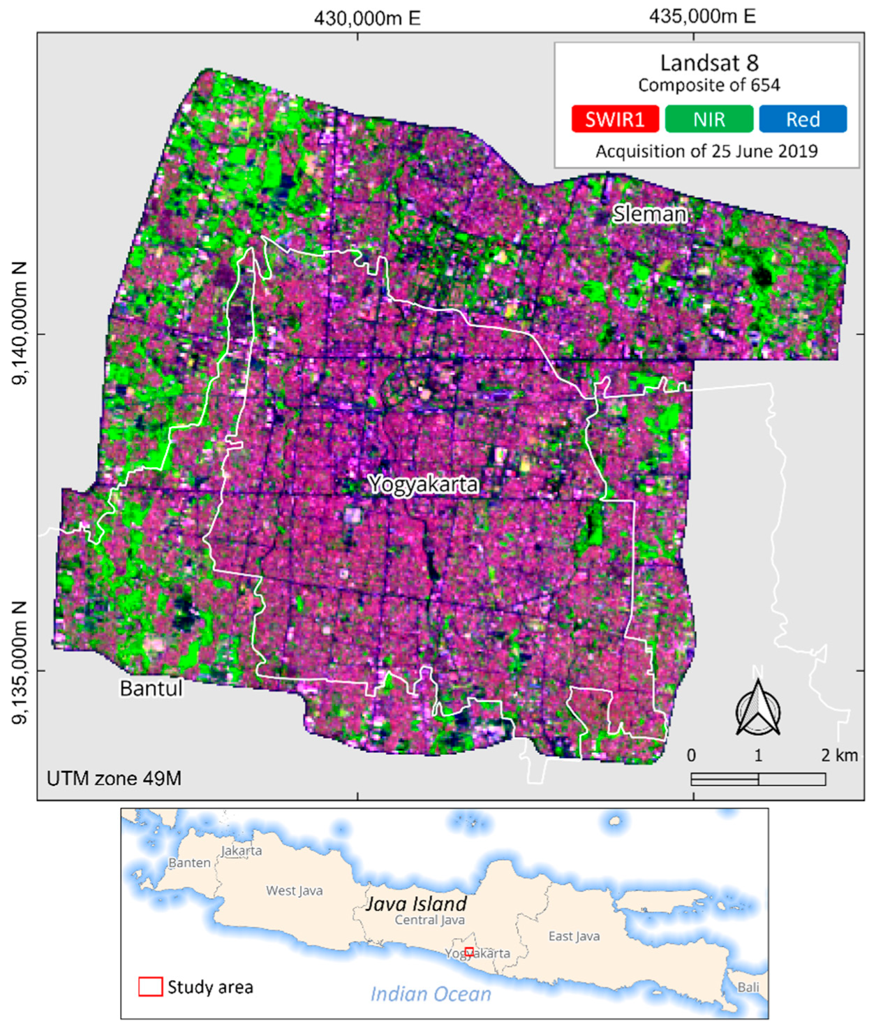
2. Study Area
3. Materials and Methods
3.1. Landsat Data and Pre-Processing
3.2. Building Datasets
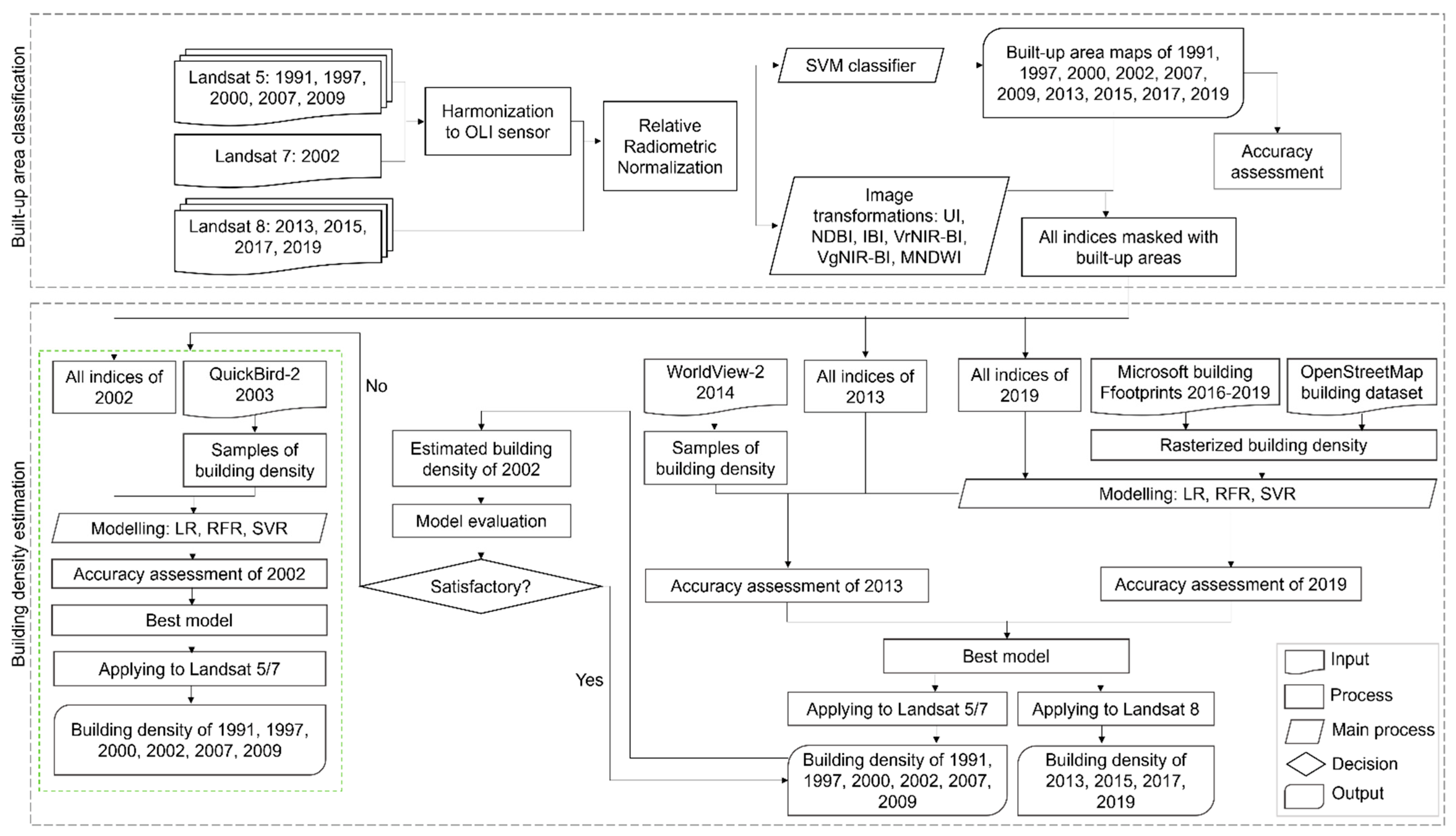
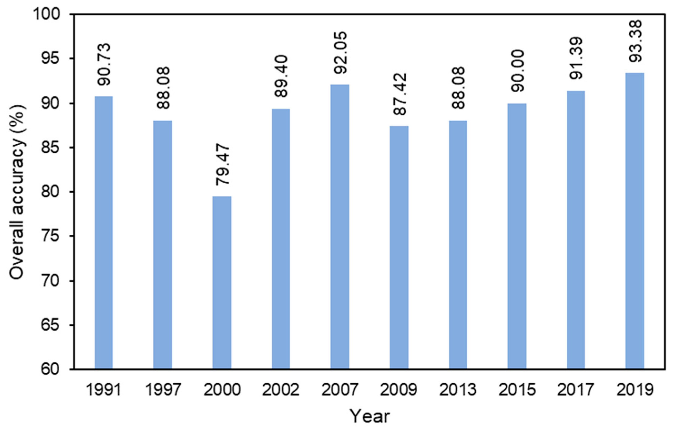
3.3. Built-Up Area Classification
3.4. Building Density Extraction
4. Results
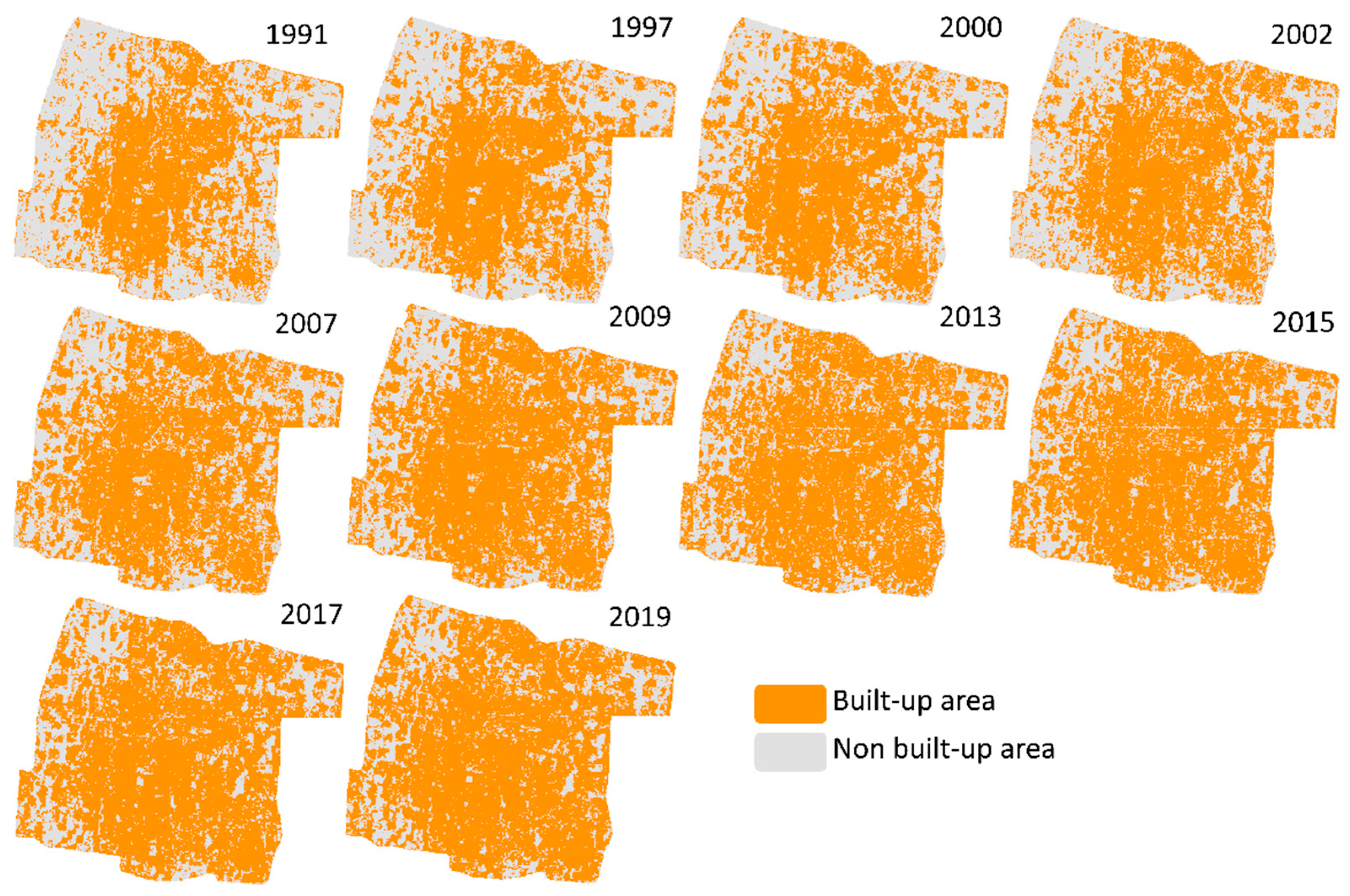
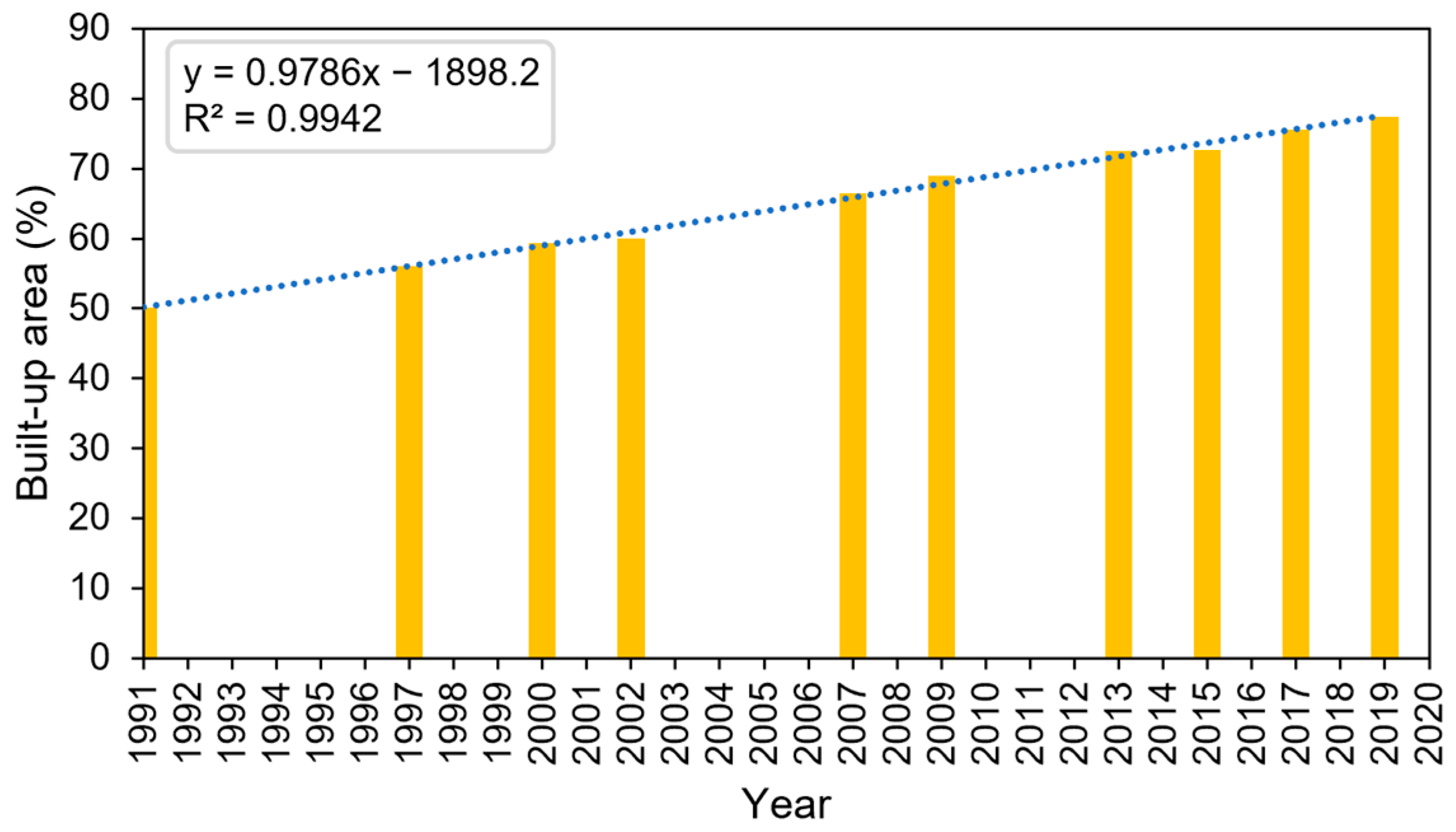
4.1. Transformation of the Built-Up Area
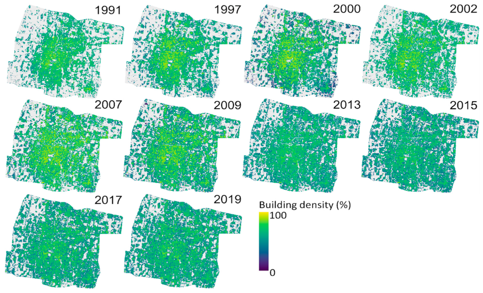
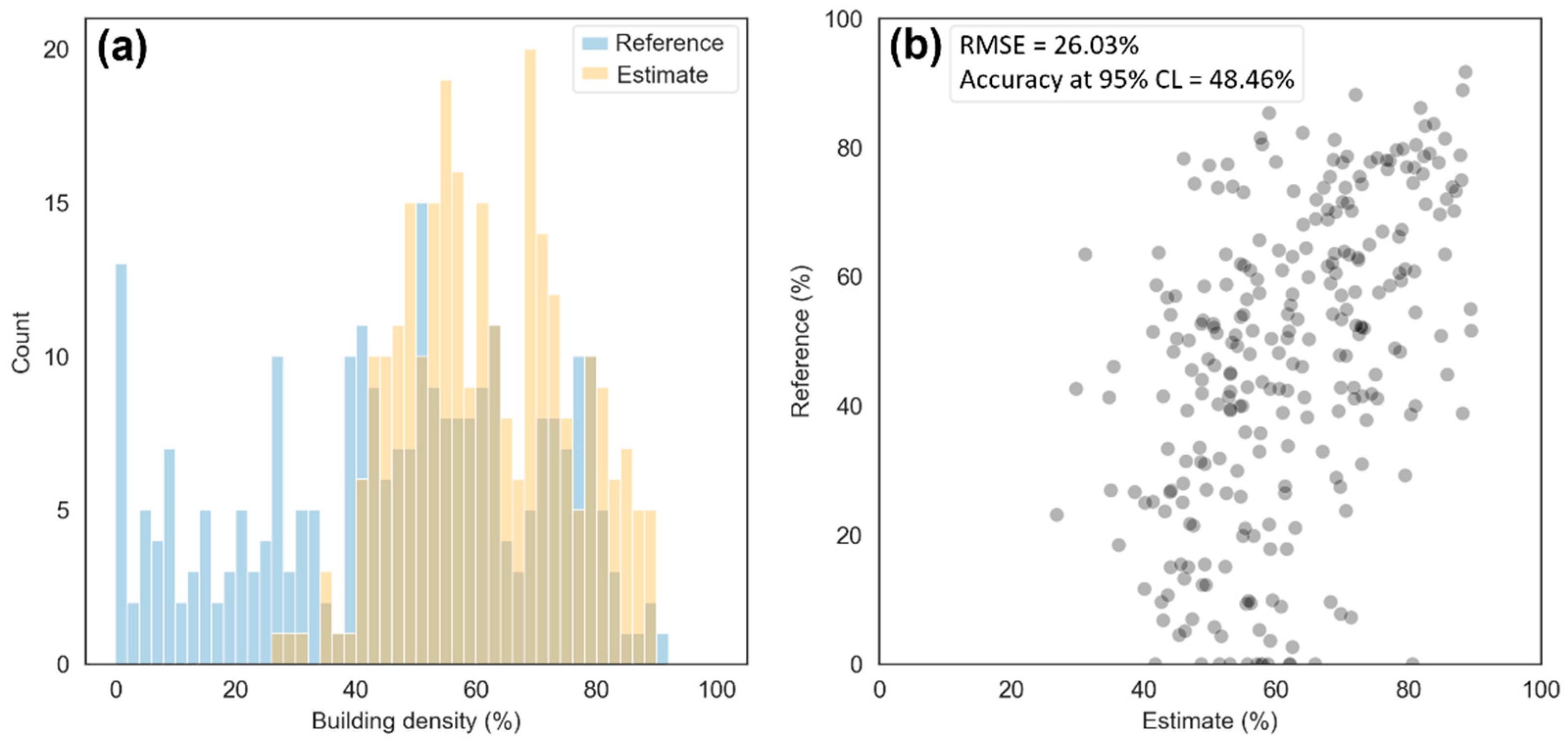
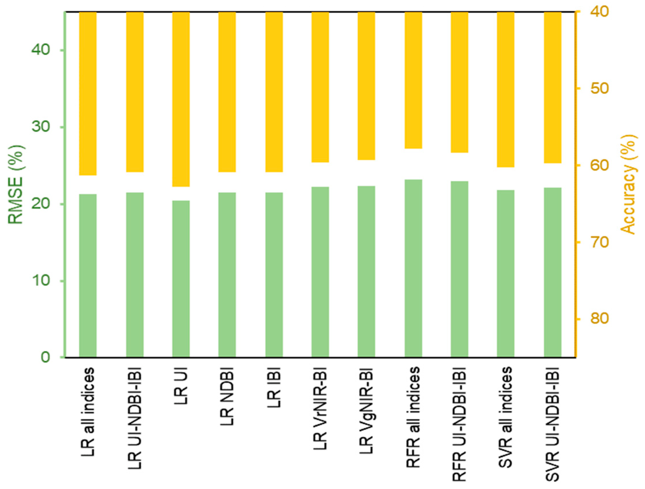
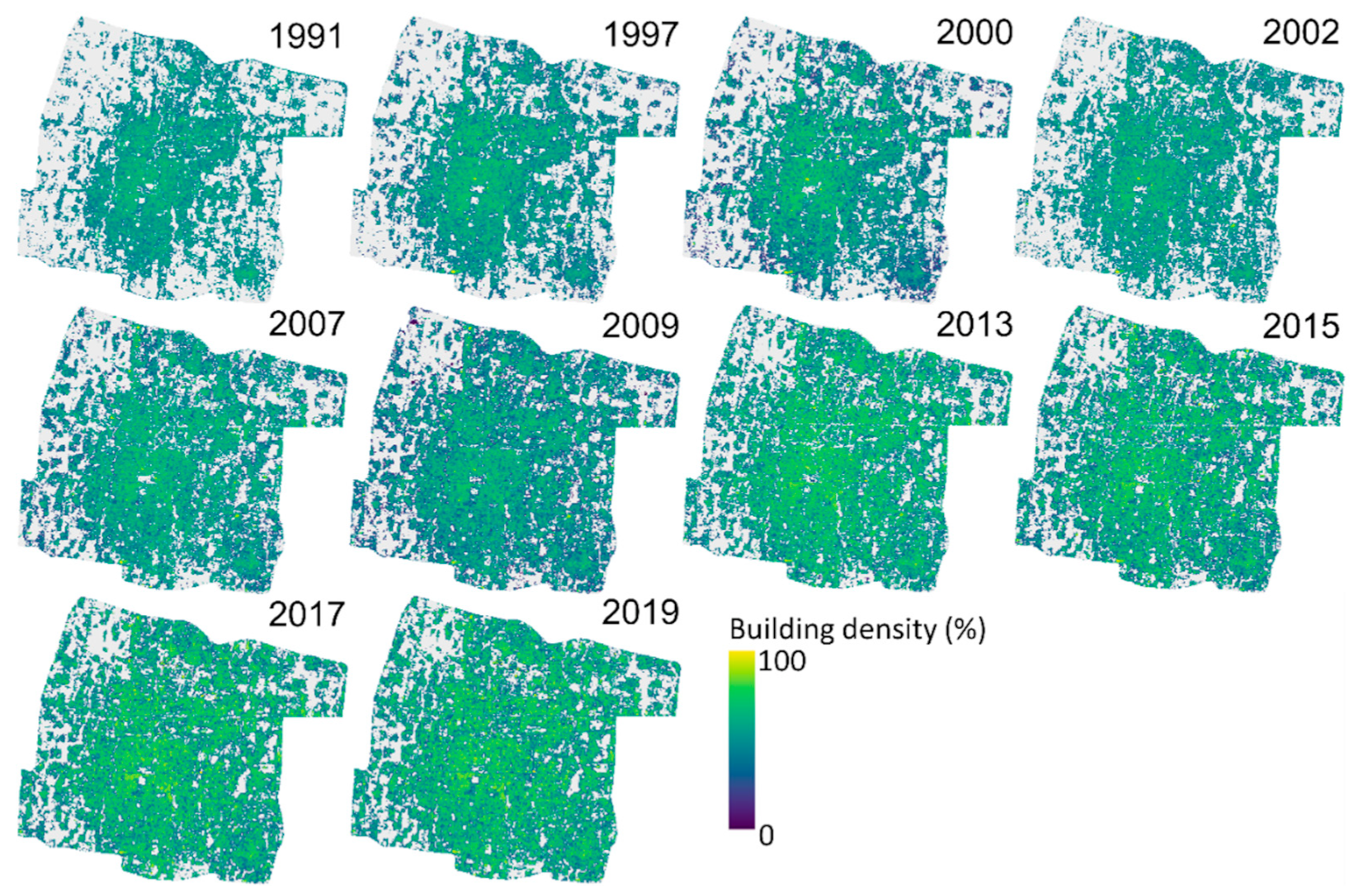
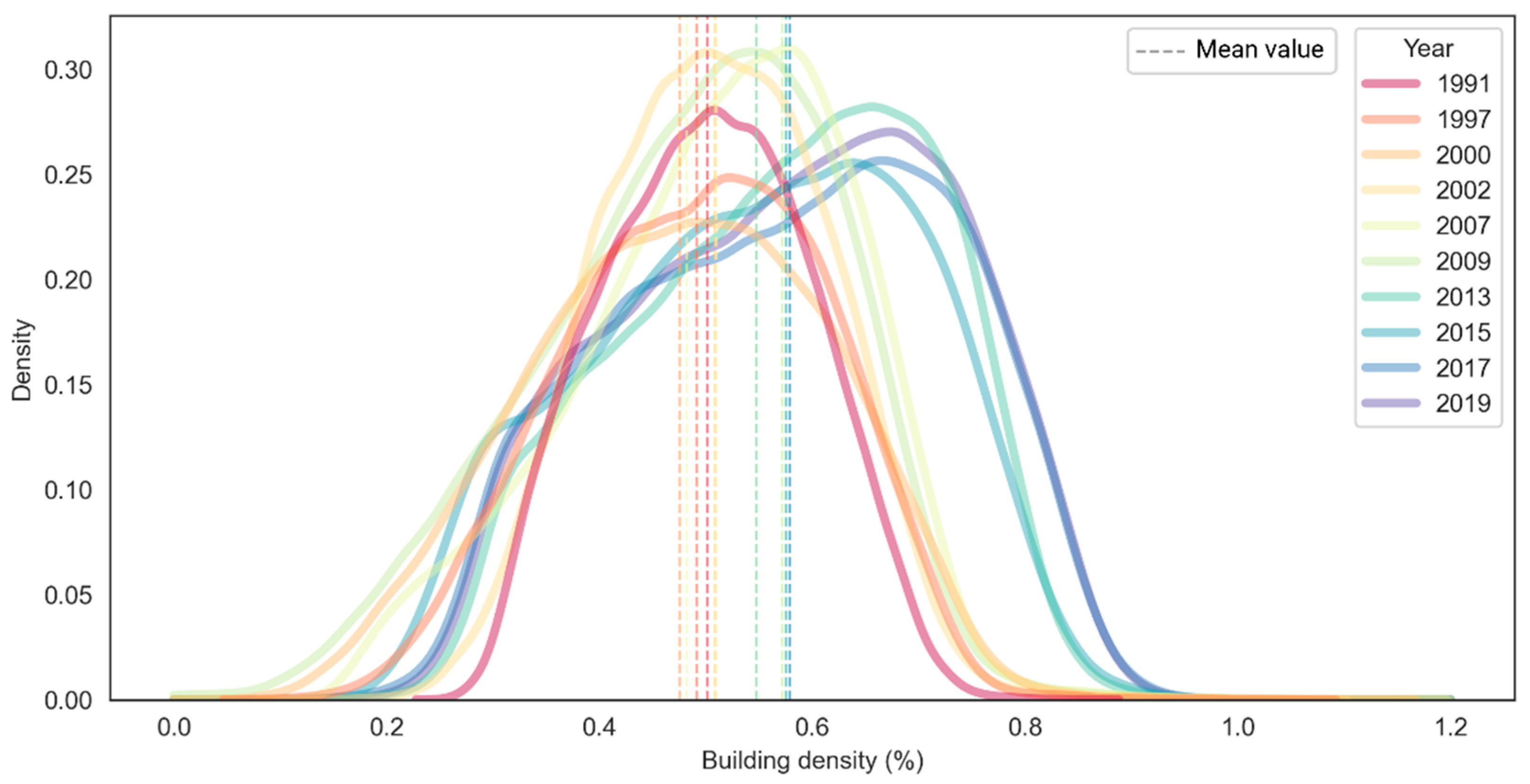
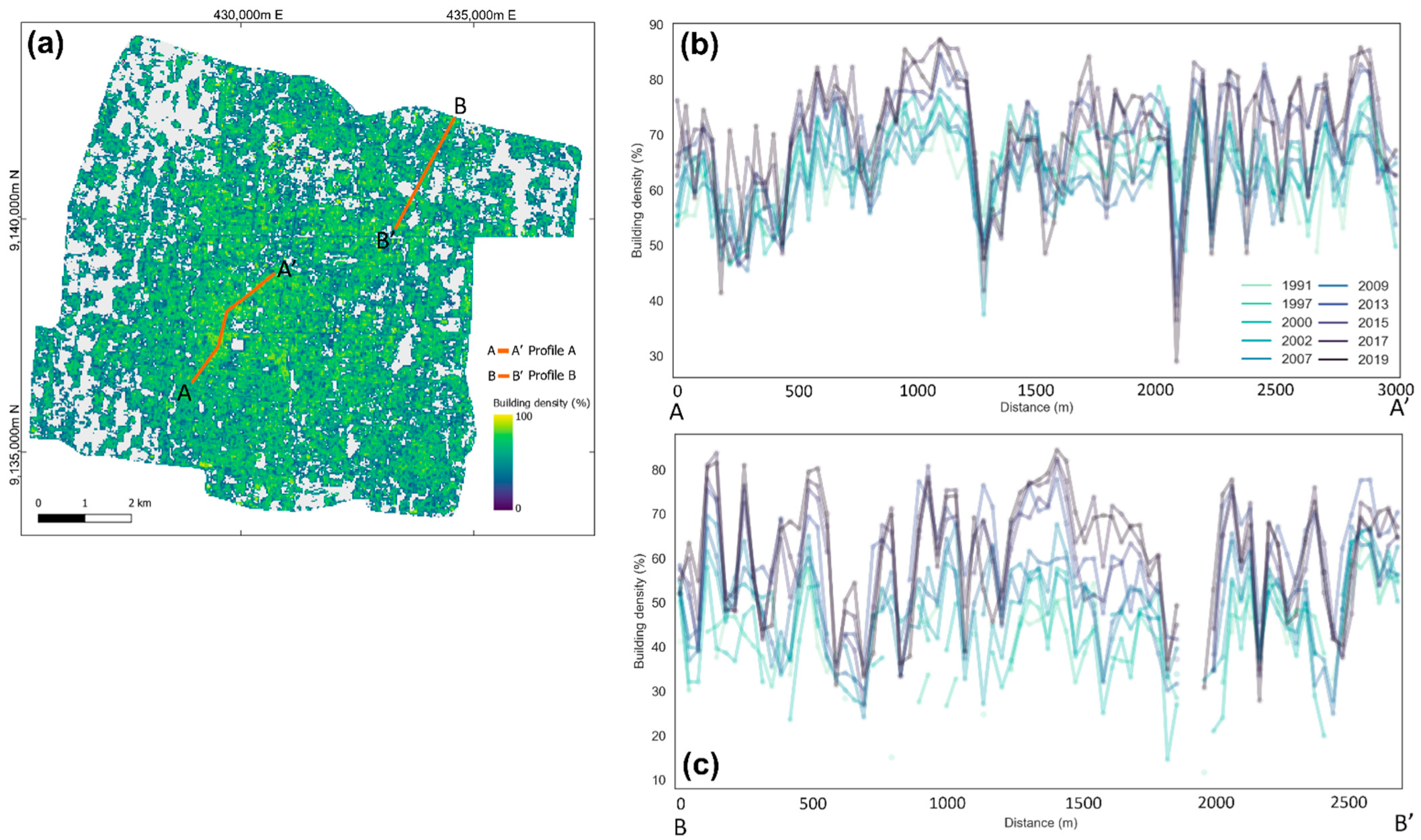
4.2. Building Density Estimation
5. Discussion
5.1. Multiple Landsat Sensors for Decadal Modeling
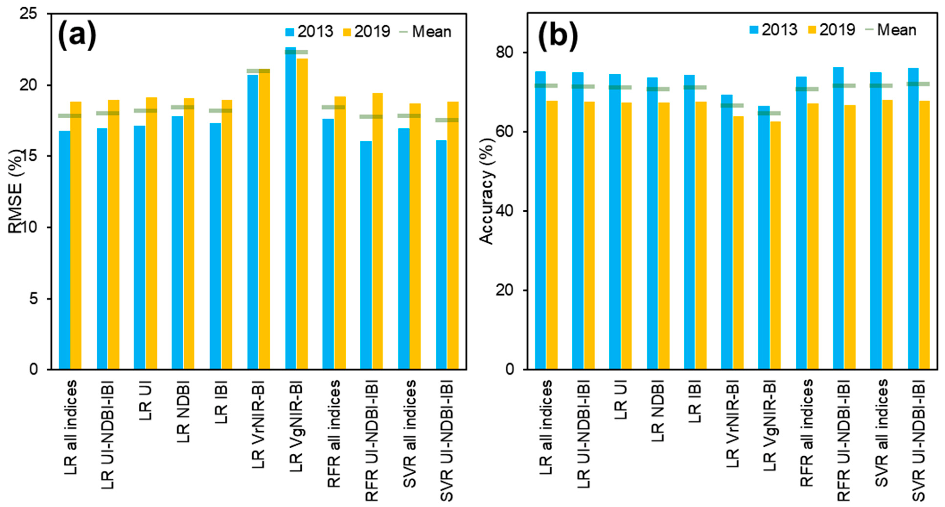
5.2. Comparison of Regression Algorithms
5.3. Expansion and Densification of Built-Up Area
6. Conclusions
Author Contributions
Funding
Institutional Review Board Statement
Informed Consent Statement
Data Availability Statement
Acknowledgments
Conflicts of Interest
Appendix A

| No. | Dataset | Bands | |||||
|---|---|---|---|---|---|---|---|
| Blue | Green | Red | NIR | SWIR1 | SWIR2 | ||
| 1 | Landsat 5—1991 | 0.8039 | 0.8163 | 0.8185 | 0.8531 | 0.8547 | 0.8679 |
| 2 | Landsat 5—1997 | 0.8854 | 0.8230 | 0.8675 | 0.8322 | 0.9127 | 0.9084 |
| 3 | Landsat 5—2000 | 0.8952 | 0.8766 | 0.8944 | 0.8817 | 0.9323 | 0.9207 |
| 4 | Landsat 7—2002 | 0.8080 | 0.8236 | 0.8046 | 0.8752 | 0.8693 | 0.8890 |
| 5 | Landsat 5—2007 | 0.9516 | 0.9629 | 0.9399 | 0.9500 | 0.9169 | 0.9231 |
| 6 | Landsat 8—2013 | 0.6901 | 0.7554 | 0.8000 | 0.8578 | 0.6905 | 0.6865 |
| 7 | Landsat 8—2015 | 0.8658 | 0.9496 | 0.9329 | 0.9345 | 0.8694 | 0.8501 |
| 8 | Landsat 8—2017 | 0.8816 | 0.9386 | 0.9328 | 0.9447 | 0.8895 | 0.8668 |
| 9 | Landsat 8—2019 | 0.8732 | 0.9567 | 0.9329 | 0.9438 | 0.9115 | 0.8790 |
References
- Acuto, M.; Parnell, S.; Seto, K.C. Building a Global Urban Science. Nat. Sustain. 2018, 1, 2–4. [Google Scholar] [CrossRef]
- Andersson, E.; Colding, J. Understanding How Built Urban Form Influences Biodiversity. Urban For. Urban Green. 2014, 13, 221–226. [Google Scholar] [CrossRef]
- Oliveira, V. Urban Morphology. J. Urban. 2008, 1, 91–96. [Google Scholar] [CrossRef]
- Zhu, Z.; Zhou, Y.; Seto, K.C.; Stokes, E.C.; Deng, C.; Pickett, S.T.A.; Taubenböck, H. Understanding an Urbanizing Planet: Strategic Directions for Remote Sensing. Remote Sens. Environ. 2019, 228, 164–182. [Google Scholar] [CrossRef]
- Duranton, G.; Puga, D. The Economics of Urban Density. J. Econ. Perspect. 2020, 34, 3–26. [Google Scholar] [CrossRef]
- Cetin, M. The Effect of Urban Planning on Urban Formations Determining Bioclimatic Comfort Area’s Effect Using Satellitia Imagines on Air Quality: A Case Study of Bursa City. Air Qual. Atmos. Health 2019, 12, 1237–1249. [Google Scholar] [CrossRef]
- Grafius, D.R.; Corstanje, R.; Harris, J.A. Linking Ecosystem Services, Urban Form and Green Space Configuration Using Multivariate Landscape Metric Analysis. Landsc. Ecol. 2018, 33, 557–573. [Google Scholar] [CrossRef]
- Indrawati, L.; Sigit Heru Murti, B.S.; Rachmawati, R.; Aji, D.S. Effect of Urban Expansion Intensity on Urban Ecological Status Utilizing Remote Sensing and GIS: A Study of Semarang-Indonesia. In IOP Conference Series: Earth and Environmental Science, Proceedings of the 3rd Environmental Resources Management in Global Region, Universitas Gadjah Mada-Yogyakarta, Indonesia, 14 November 2019; IOP Publishing Ltd.: Bristol, UK, 2020; Volume 451, p. 012018. [Google Scholar] [CrossRef]
- Sahana, M.; Hong, H.; Sajjad, H. Analyzing Urban Spatial Patterns and Trend of Urban Growth Using Urban Sprawl Matrix: A Study on Kolkata Urban Agglomeration, India. Sci. Total Environ. 2018, 628–629, 1557–1566. [Google Scholar] [CrossRef]
- Krehl, A.; Siedentop, S.; Taubenböck, H.; Wurm, M. A Comprehensive View on Urban Spatial Structure: Urban Density Patterns of German City Regions. ISPRS Int. J. Geo-Inf. 2016, 5, 76. [Google Scholar] [CrossRef]
- Cetin, M.; Adiguzel, F.; Gungor, S.; Kaya, E.; Sancar, M.C. Evaluation of Thermal Climatic Region Areas in Terms of Building Density in Urban Management and Planning for Burdur, Turkey. Air Qual. Atmos. Health 2019, 12, 1103–1112. [Google Scholar] [CrossRef]
- Lin, P.; Lau, S.S.Y.; Qin, H.; Gou, Z. Effects of Urban Planning Indicators on Urban Heat Island: A Case Study of Pocket Parks in High-Rise High-Density Environment. Landsc. Urban Plan. 2017, 168, 48–60. [Google Scholar] [CrossRef]
- Güneralp, B.; Zhou, Y.; Ürge-Vorsatz, D.; Gupta, M.; Yu, S.; Patel, P.L.; Fragkias, M.; Li, X.; Seto, K.C. Global Scenarios of Urban Density and Its Impacts on Building Energy Use through 2050. Proc. Natl. Acad. Sci. USA 2017, 114, 8945–8950. [Google Scholar] [CrossRef] [PubMed]
- Resch, E.; Bohne, R.A.; Kvamsdal, T.; Lohne, J. Impact of Urban Density and Building Height on Energy Use in Cities. Energy Procedia 2016, 96, 800–814. [Google Scholar] [CrossRef]
- Sallis, J.F.; Cerin, E.; Conway, T.L.; Adams, M.A.; Frank, L.D.; Pratt, M.; Salvo, D.; Schipperijn, J.; Smith, G.; Cain, K.L.; et al. Physical Activity in Relation to Urban Environments in 14 Cities Worldwide: A Cross-Sectional Study. Lancet 2016, 387, 2207–2217. [Google Scholar] [CrossRef]
- Song, J.; Chen, W.; Zhang, J.; Huang, K.; Hou, B.; Prishchepov, A.V. Effects of Building Density on Land Surface Temperature in China: Spatial Patterns and Determinants. Landsc. Urban Plan. 2020, 198, 103794. [Google Scholar] [CrossRef]
- Emmanuel, R.; Steemers, K. Connecting the Realms of Urban Form, Density and Microclimate. Build. Res. Inf. 2018, 46, 804–808. [Google Scholar] [CrossRef]
- Gabriel, K.M.A.; Endlicher, W.R. Urban and Rural Mortality Rates during Heat Waves in Berlin and Brandenburg, Germany. Environ. Pollut. 2011, 159, 2044–2050. [Google Scholar] [CrossRef]
- Li, Y.; Schubert, S.; Kropp, J.P.; Rybski, D. On the Influence of Density and Morphology on the Urban Heat Island Intensity. Nat. Commun. 2020, 11, 2647. [Google Scholar] [CrossRef]
- Soltani, A.; Sharifi, E. Daily Variation of Urban Heat Island Effect and Its Correlations to Urban Greenery: A Case Study of Adelaide. Front. Archit. Res. 2017, 6, 529–538. [Google Scholar] [CrossRef]
- Ahmadian, E.; Sodagar, B.; Mills, G.; Byrd, H.; Bingham, C.; Zolotas, A. Sustainable Cities: The Relationships between Urban Built Forms and Density Indicators. Cities 2019, 95, 102382. [Google Scholar] [CrossRef]
- Susanti, R.; Soetomo, S.; Buchori, I.; Brotosunaryo, P.M. Smart Growth, Smart City and Density: In Search of The Appropriate Indicator for Residential Density in Indonesia. Procedia Soc. Behav. Sci. 2016, 227, 194–201. [Google Scholar] [CrossRef]
- Farrell, K. The Rapid Urban Growth Triad: A New Conceptual Framework for Examining the Urban Transition in Developing Countries. Sustainability 2017, 9, 1407. [Google Scholar] [CrossRef]
- Li, X.; Gong, P. Urban Growth Models: Progress and Perspective. Sci. Bull. 2016, 61, 1637–1650. [Google Scholar] [CrossRef]
- Sun, C.; Hu, W. A Rapid Building Density Survey Method Based on Improved Unet. In Proceedings of the 25th CAADRIA Conference, Bangkok, Thailand, 5–6 August 2020; Volume 2, pp. 649–658. [Google Scholar]
- Zhu, Z.; Wulder, M.A.; Roy, D.P.; Woodcock, C.E.; Hansen, M.C.; Radeloff, V.C.; Healey, S.P.; Schaaf, C.; Hostert, P.; Strobl, P.; et al. Benefits of the Free and Open Landsat Data Policy. Remote Sens. Environ. 2019, 224, 382–385. [Google Scholar] [CrossRef]
- Wulder, M.A.; White, J.C.; Loveland, T.R.; Woodcock, C.E.; Belward, A.S.; Cohen, W.B.; Fosnight, E.A.; Shaw, J.; Masek, J.G.; Roy, D.P. The Global Landsat Archive: Status, Consolidation, and Direction. Remote Sens. Environ. 2016, 185, 271–283. [Google Scholar] [CrossRef]
- Nguyen, G.C.; Dang, K.V.; Vu, T.A.; Nguyen, A.K.; Weber, C. Ha Long—Cam Pha Cities Evolution Analysis Utilizing Remote Sensing Data. Remote Sens. 2022, 14, 1241. [Google Scholar] [CrossRef]
- Pu, R.; Landry, S. A Comparative Analysis of High Spatial Resolution IKONOS and WorldView-2 Imagery for Mapping Urban Tree Species. Remote Sens. Environ. 2012, 124, 516–533. [Google Scholar] [CrossRef]
- Wulder, M.A.; Masek, J.G.; Cohen, W.B.; Loveland, T.R.; Woodcock, C.E. Opening the Archive: How Free Data Has Enabled the Science and Monitoring Promise of Landsat. Remote Sens. Environ. 2012, 122, 2–10. [Google Scholar] [CrossRef]
- Wulder, M.A.; Loveland, T.R.; Roy, D.P.; Crawford, C.J.; Masek, J.G.; Woodcock, C.E.; Allen, R.G.; Anderson, M.C.; Belward, A.S.; Cohen, W.B.; et al. Current Status of Landsat Program, Science, and Applications. Remote Sens. Environ. 2019, 225, 127–147. [Google Scholar] [CrossRef]
- Chen, X.-L.; Zhao, H.-M.; Li, P.-X.; Yin, Z.-Y. Remote Sensing Image-Based Analysis of the Relationship between Urban Heat Island and Land Use/Cover Changes. Remote Sens. Environ. 2006, 104, 133–146. [Google Scholar] [CrossRef]
- Kim, S.W.; Brown, R.D. Urban Heat Island (UHI) Variations within a City Boundary: A Systematic Literature Review. Renew. Sustain. Energy Rev. 2021, 148, 111256. [Google Scholar] [CrossRef]
- Monteiro, F.F.; Gonçalves, W.A.; Andrade, L.; de Melo Barbosa Andrade, L.; Villavicencio, L.M.M.; dos Santos Silva, C.M. Assessment of Urban Heat Islands in Brazil Based on MODIS Remote Sensing Data. Urban Clim. 2021, 35, 100726. [Google Scholar] [CrossRef]
- As-syakur, A.R.; Adnyana, I.W.S.; Arthana, I.W.; Nuarsa, I.W. Enhanced Built-UP and Bareness Index (EBBI) for Mapping Built-UP and Bare Land in an Urban Area. Remote Sens. 2012, 4, 2957–2970. [Google Scholar] [CrossRef]
- Ghosh, D.K.; Mandal, A.C.H.; Majumder, R.; Patra, P.; Bhunia, G.S. Analysis for Mapping of Built-up Area Using Remotely Sensed Indices—A Case Study of Rajarhat Block in Barasat Sadar Sub-Division in West Bengal (India). J. Landsc. Ecol. 2018, 11, 67–76. [Google Scholar] [CrossRef]
- Kawamura, M.; Jayamanna, S.; Tsujiko, Y. Relation Between Social and Environmental Condition in Colombo, Sri Lanka and The Urban Index Estimated by Satellite Remote Sensing Data. Int. Arch. Photogramm. Remote Sens. 1996, 31, 321–326. [Google Scholar]
- Zha, Y.; Gao, J.; Ni, S. Use of Normalized Difference Built-up Index in Automatically Mapping Urban Areas from TM Imagery. Int. J. Remote Sens. 2003, 24, 583–594. [Google Scholar] [CrossRef]
- Xu, H. A New Index for Delineating Built-up Land Features in Satellite Imagery. Int. J. Remote Sens. 2008, 29, 4269–4276. [Google Scholar] [CrossRef]
- Estoque, R.C.; Murayama, Y. Classification and Change Detection of Built-up Lands from Landsat-7 ETM+ and Landsat-8 OLI/TIRS Imageries: A Comparative Assessment of Various Spectral Indices. Ecol. Indic. 2015, 56, 205–217. [Google Scholar] [CrossRef]
- Bhatti, S.S.; Tripathi, N.K. Built-up Area Extraction Using Landsat 8 OLI Imagery. GISci. Remote Sens. 2014, 51, 445–467. [Google Scholar] [CrossRef]
- Zhang, Q.; Wang, J.; Peng, X.; Gong, P.; Shi, P. Urban Built-up Land Change Detection with Road Density and Spectral Information from Multi-Temporal Landsat TM Data. Int. J. Remote Sens. 2002, 23, 3057–3078. [Google Scholar] [CrossRef]
- Handayani, H.H.; Murayama, Y.; Ranagalage, M.; Liu, F.; Dissanayake, D.M.S.L.B. Geospatial Analysis of Horizontal and Vertical Urban Expansion Using Multi-Spatial Resolution Data: A Case Study of Surabaya, Indonesia. Remote Sens. 2018, 10, 1599. [Google Scholar] [CrossRef]
- Xia, C.; Yeh, A.G.O.; Zhang, A. Analyzing Spatial Relationships between Urban Land Use Intensity and Urban Vitality at Street Block Level: A Case Study of Five Chinese Megacities. Landsc. Urban Plan. 2020, 193, 103669. [Google Scholar] [CrossRef]
- Xi, Y.; Thinh, N.X.; Li, C. Preliminary Comparative Assessment of Various Spectral Indices for Built-up Land Derived from Landsat-8 OLI and Sentinel-2A MSI Imageries. Eur. J. Remote Sens. 2019, 52, 240–252. [Google Scholar] [CrossRef]
- Ghanea, M.; Moallem, P.; Momeni, M. Building Extraction from High-Resolution Satellite Images in Urban Areas: Recent Methods and Strategies against Significant Challenges. Int. J. Remote Sens. 2016, 37, 5234–5248. [Google Scholar] [CrossRef]
- Zhang, T.; Huang, X.; Wen, D.; Li, J. Urban Building Density Estimation from High-Resolution Imagery Using Multiple Features and Support Vector Regression. IEEE J. Sel. Top. Appl. Earth Obs. Remote Sens. 2017, 10, 3265–3280. [Google Scholar] [CrossRef]
- Heinzel, J.; Kemper, T. Automated Metric Characterization of Urban Structure Using Building Decomposition from Very High Resolution Imagery. Int. J. Appl. Earth Obs. Geoinf. 2015, 35, 151–160. [Google Scholar] [CrossRef]
- Shahfahad; Mourya, M.; Kumari, B.; Tayyab, M.; Paarcha, A.; Asif; Rahman, A. Indices Based Assessment of Built-up Density and Urban Expansion of Fast Growing Surat City Using Multi-Temporal Landsat Data Sets. GeoJournal 2021, 86, 1607–1623. [Google Scholar] [CrossRef]
- Ehrlich, D.; Kemper, T.; Pesaresi, M.; Corbane, C. Built-up Area and Population Density: Two Essential Societal Variables to Address Climate Hazard Impact. Environ. Sci. Policy 2018, 90, 73–82. [Google Scholar] [CrossRef]
- Elmdari, Y.; Namir, A.; Hakdaoui, M. Analysis of Urban Growth and Sprawl and Built Up Density Using Remote Sensing Data: Case of Casablanca, Morocco. Int. J. Adv. Res. 2018, 6, 1107–1116. [Google Scholar] [CrossRef]
- Asyraf, M.S.; Damayanti, A.; Dimyati, M. The Effect of Building Density on Land Surface Temperature, (Case Study: Turikale District, Maros Regency). In IOP Conference Series: Earth and Environmental Science, Proceedings of the Fifth International Conferences of Indonesian Society for Remote Sensing, West Java, Indonesia, 17–20 September 2019; IOP Publishing Ltd.: Bristol, UK, 2020; Volume 500, p. 012061. [Google Scholar] [CrossRef]
- Ridwan; Rasyidi, E.S.; Syafri; Rahman, R.; Okviyani, N.; Jumadil; Ma’rief, A.A. Assessment of the Relationship between Building Density and Urban Heat Island Using Landsat Images in Makassar City. In IOP Conference Series: Earth and Environmental Science, Proceedings of the International Conference on Research Collaboration of Environmental Science, Kitakyushu, Japan, 25–26 April 2021; IOP Publishing Ltd.: Bristol, UK, 2021; Volume 802, p. 012042. [Google Scholar] [CrossRef]
- Ardiansyah; Hernina, R.; Suseno, W.; Zulkarnain, F.; Yanidar, R.; Rokhmatuloh, R. Percent of Building Density (PBD) of Urban Environment: A Multi-Index Approach Based Study in DKI Jakarta Province. Indones. J. Geogr. 2019, 50, 154–161. [Google Scholar] [CrossRef]
- Risky, Y.S.; Aulia, Y.H.; Widayani, P. Spatiotemporal Built-up Land Density Mapping Using Various Spectral Indices in Landsat-7 ETM+ and Landsat-8 OLI/TIRS (Case Study: Surakarta City). In IOP Conference Series: Earth and Environmental Science, Proceedings of the 5th Geoinformation Science Symposium 2017 (GSS 2017), Yogyakarta, Indonesia, 27–28 September 2017; IOP Publishing Ltd.: Bristol, UK, 2017; Volume 98, p. 012006. [Google Scholar] [CrossRef]
- Chen, J.; de Hoogh, K.; Gulliver, J.; Hoffmann, B.; Hertel, O.; Ketzel, M.; Bauwelinck, M.; van Donkelaar, A.; Hvidtfeldt, U.A.; Katsouyanni, K.; et al. A Comparison of Linear Regression, Regularization, and Machine Learning Algorithms to Develop Europe-Wide Spatial Models of Fine Particles and Nitrogen Dioxide. Environ. Int. 2019, 130, 104934. [Google Scholar] [CrossRef] [PubMed]
- Jumin, E.; Zaini, N.; Ahmed, A.N.; Abdullah, S.; Ismail, M.; Sherif, M.; Sefelnasr, A.; El-Shafie, A. Machine Learning versus Linear Regression Modelling Approach for Accurate Ozone Concentrations Prediction. Eng. Appl. Comput. Fluid Mech. 2020, 14, 713–725. [Google Scholar] [CrossRef]
- Rozano, B.; Yan, W. Monitoring the Transformation of Yogyakarta’s Urban Form Using Remote Sensing and Geographic Information System. In IOP Conference Series: Earth and Environmental Science, Proceedings of the International Conference on Environmental Resources Management in Global Region (ICERM 2017), Bali, Indonesia, 25 November 2017; IOP Publishing Ltd.: Bristol, UK, 2018; Volume 148, p. 012010. [Google Scholar] [CrossRef]
- Schmidt, G.L.; Jenkerson, C.B.; Masek, J.; Vermote, E.; Gao, F. Landsat Ecosystem Disturbance Adaptive Processing System (LEDAPS) Algorithm Description; U.S. Geological Survey Open-File Report; USGS: Reston, VA, USA, 2013. [Google Scholar]
- Vermote, E.; Justice, C.; Claverie, M.; Franch, B. Preliminary Analysis of the Performance of the Landsat 8/OLI Land Surface Reflectance Product. Remote Sens. Environ. 2016, 185, 46–56. [Google Scholar] [CrossRef] [PubMed]
- Foga, S.; Scaramuzza, P.L.; Guo, S.; Zhu, Z.; Dilley, R.D.; Beckmann, T.; Schmidt, G.L.; Dwyer, J.L.; Joseph Hughes, M.; Laue, B. Cloud Detection Algorithm Comparison and Validation for Operational Landsat Data Products. Remote Sens. Environ. 2017, 194, 379–390. [Google Scholar] [CrossRef]
- Roy, D.P.; Kovalskyy, V.; Zhang, H.K.; Vermote, E.F.; Yan, L.; Kumar, S.S.; Egorov, A. Characterization of Landsat-7 to Landsat-8 Reflective Wavelength and Normalized Difference Vegetation Index Continuity. Remote Sens. Environ. 2016, 185, 57–70. [Google Scholar] [CrossRef]
- Young, N.E.; Anderson, R.S.; Chignell, S.M.; Vorster, A.G.; Lawrence, R.; Evangelista, P.H. A Survival Guide to Landsat Preprocessing. Ecology 2017, 98, 920–932. [Google Scholar] [CrossRef]
- Yang, X.; Lo, C.P. Relative Radiometric Normalization Performance for Change Detection from Multi-Date Satellite Images. Photogramm. Eng. Remote. Sens. 2000, 66, 967–980. [Google Scholar]
- Du, Y.; Teillet, P.M.; Cihlar, J. Radiometric Normalization of Multitemporal High-Resolution Satellite Images with Quality Control for Land Cover Change Detection. Remote Sens. Environ. 2002, 82, 123–134. [Google Scholar] [CrossRef]
- Microsoft. Indonesia, Malaysia, and Philipines Building Footprints. Available online: https://github.com/microsoft/IdMyPhBuildingFootprints (accessed on 11 April 2022).
- Heris, M.P.; Foks, N.L.; Bagstad, K.J.; Troy, A.; Ancona, Z.H. A Rasterized Building Footprint Dataset for the United States. Sci. Data 2020, 7, 207. [Google Scholar] [CrossRef]
- Karasiak, N. Dzetsaka Qgis Classification Plugin. Available online: https://github.com/nkarasiak/dzetsaka (accessed on 10 June 2022).
- Pal, M.; Mather, P.M. Support Vector Machines for Classification in Remote Sensing. Int. J. Remote Sens. 2005, 26, 1007–1011. [Google Scholar] [CrossRef]
- Vapnik, V.N. The Nature of Statistical Learning Theory; Springer: New York, NY, USA, 2000; ISBN 978-1-4419-3160-3. [Google Scholar]
- Van der Linden, S.; Rabe, A.; Held, M.; Jakimow, B.; Leitão, P.; Okujeni, A.; Schwieder, M.; Suess, S.; Hostert, P. The EnMAP-Box—A Toolbox and Application Programming Interface for EnMAP Data Processing. Remote Sens. 2015, 7, 11249–11266. [Google Scholar] [CrossRef]
- Segal, M.R. Machine Learning Benchmarks and Random Forest Regression Publication Date Machine Learning Benchmarks and Random Forest Regression. Cent. Bioinform. Mol. Biostat. 2004, 15, 1–15. [Google Scholar]
- Mountrakis, G.; Im, J.; Ogole, C. Support Vector Machines in Remote Sensing: A Review. ISPRS J. Photogramm. Remote Sens. 2011, 66, 247–259. [Google Scholar] [CrossRef]
- Shafizadeh-Moghadam, H.; Tayyebi, A.; Ahmadlou, M.; Delavar, M.R.; Hasanlou, M. Integration of Genetic Algorithm and Multiple Kernel Support Vector Regression for Modeling Urban Growth. Comput. Environ. Urban Syst. 2017, 65, 28–40. [Google Scholar] [CrossRef]
- Wicaksono, P.; Danoedoro, P.; Hartono, H.; Nehren, U.; Ribbe, L. Preliminary Work of Mangrove Ecosystem Carbon Stock Mapping in Small Island Using Remote Sensing: Above and below Ground Carbon Stock Mapping on Medium Resolution Satellite Image. In Remote Sensing for Agriculture, Ecosystems, and Hydrology XIII; Neale, C.M.U., Maltese, A., Eds.; SPIE: Prague, Czech Republic, 2011; p. 81741B. [Google Scholar]
- Taati, A.; Sarmadian, F.; Mousavi, A.; Taghati, C.; Pour, H.; Shahir, A.H.E. Land Use Classification Using Support Vector Machine and Maximum Likelihood Algorithms by Landsat 5 TM Images. Walailak-J. Sci. Technol. 2015, 12, 681–687. [Google Scholar] [CrossRef]
- Shi, D.; Yang, X. Support Vector Machines for Land Cover Mapping from Remote Sensor Imagery. In Monitoring and Modeling of Global Changes: A Geomatics Perspective; Li, J., Yang, X., Eds.; Springer: Dordrecht, The Netherlands, 2015; pp. 265–279. ISBN 978-94-017-9812-9/978-94-017-9813-6. [Google Scholar]
- Ma, X.; Tong, X.; Liu, S.; Luo, X.; Xie, H.; Li, C. Optimized Sample Selection in SVM Classification by Combining with DMSP-OLS, Landsat NDVI and GlobeLand30 Products for Extracting Urban Built-Up Areas. Remote Sens. 2017, 9, 236. [Google Scholar] [CrossRef]
- Mukherjee, A.; Kumar, A.A.; Ramachandran, P. Development of New Index-Based Methodology for Extraction of Built-Up Area From Landsat7 Imagery: Comparison of Performance With SVM, ANN, and Existing Indices. IEEE Trans. Geosci. Remote Sens. 2021, 59, 1592–1603. [Google Scholar] [CrossRef]
- Mathur, A.; Foody, G.M. Land Cover Classification by Support Vector Machine: Towards Efficient Training. In Proceedings of the IEEE International Geoscience and Remote Sensing Symposium, Anchorage, AK, USA, 20–24 September 2004; Volume 2, pp. 742–744. [Google Scholar]
- Osgouei, P.E.; Kaya, S.; Sertel, E.; Alganci, U. Separating Built-up Areas from Bare Land in Mediterranean Cities Using Sentinel-2A Imagery. Remote Sens. 2019, 11, 345. [Google Scholar] [CrossRef]
- Feng, S.; Fan, F. Impervious Surface Extraction Based on Different Methods from Multiple Spatial Resolution Images: A Comprehensive Comparison. Int. J. Digit. Earth 2021, 14, 1148–1174. [Google Scholar] [CrossRef]
- Krówczyńska, M.; Soszyńska, A.; Pabjanek, P.; Wilk, E.; Hurbanek, P.; Rosina, K. Accuracy of the Soil Sealing Enhancement Product for Poland. Quaest. Geogr. 2016, 35, 89–95. [Google Scholar] [CrossRef][Green Version]
- Xu, H.; Wei, Y.; Li, X.; Zhao, Y.; Cheng, Q. A Novel Automatic Method on Pseudo-Invariant Features Extraction for Enhancing the Relative Radiometric Normalization of High-Resolution Images. Int. J. Remote Sens. 2021, 42, 6153–6183. [Google Scholar] [CrossRef]
- Zhou, H.; Liu, S.; He, J.; Wen, Q.; Song, L.; Ma, Y. A New Model for the Automatic Relative Radiometric Normalization of Multiple Images with Pseudo-Invariant Features. Int. J. Remote Sens. 2016, 37, 4554–4573. [Google Scholar] [CrossRef]
- Geng, J.; Gan, W.; Xu, J.; Yang, R.; Wang, S. Support Vector Machine Regression (SVR)-Based Nonlinear Modeling of Radiometric Transforming Relation for the Coarse-Resolution Data-Referenced Relative Radiometric Normalization (RRN). Geo-Spat. Inf. Sci. 2020, 23, 237–247. [Google Scholar] [CrossRef]
- Sadeghi, V.; Ebadi, H.; Ahmadi, F.F. A New Model for Automatic Normalization of Multitemporal Satellite Images Using Artificial Neural Network and Mathematical Methods. Appl. Math. Model. 2013, 37, 6437–6445. [Google Scholar] [CrossRef]
- Fassnacht, F.E.; Hartig, F.; Latifi, H.; Berger, C.; Hernández, J.; Corvalán, P.; Koch, B. Importance of Sample Size, Data Type and Prediction Method for Remote Sensing-Based Estimations of Aboveground Forest Biomass. Remote Sens. Environ. 2014, 154, 102–114. [Google Scholar] [CrossRef]
- Millard, K.; Richardson, M. On the Importance of Training Data Sample Selection in Random Forest Image Classification: A Case Study in Peatland Ecosystem Mapping. Remote Sens. 2015, 7, 8489–8515. [Google Scholar] [CrossRef]
- Quang, N.H.; Quinn, C.H.; Carrie, R.; Stringer, L.C.; Van Hue, L.T.; Hackney, C.R.; Van Tan, D. Comparisons of Regression and Machine Learning Methods for Estimating Mangrove Above-Ground Biomass Using Multiple Remote Sensing Data in the Red River Estuaries of Vietnam. Remote Sens. Appl. Soc. Environ. 2022, 26, 100725. [Google Scholar] [CrossRef]
- Ren, Z.; Du, Y.; He, X.; Pu, R.; Zheng, H.; Hu, H. Spatiotemporal Pattern of Urban Forest Leaf Area Index in Response to Rapid Urbanization and Urban Greening. J. For. Res. 2018, 29, 785–796. [Google Scholar] [CrossRef]
- Cai, J.; Luo, J.; Wang, S.; Yang, S. Feature Selection in Machine Learning: A New Perspective. Neurocomputing 2018, 300, 70–79. [Google Scholar] [CrossRef]
- Mahtta, R.; Fragkias, M.; Güneralp, B.; Mahendra, A.; Reba, M.; Wentz, E.A.; Seto, K.C. Urban Land Expansion: The Role of Population and Economic Growth for 300+ Cities. NPJ Urban Sustain. 2022, 2, 5. [Google Scholar] [CrossRef]
- Ying, Q.; Hansen, M.C.; Sun, L.; Wang, L.; Steininger, M. Satellite-Detected Gain in Built-up Area as a Leading Economic Indicator. Environ. Res. Lett. 2019, 14, 114015. [Google Scholar] [CrossRef]
- Chen, B.; Wu, C.; Huang, X.; Yang, X. Examining the Relationship between Urban Land Expansion and Economic Linkage Using Coupling Analysis: A Case Study of the Yangtze River Economic Belt, China. Sustainability 2020, 12, 1227. [Google Scholar] [CrossRef]
- Fang, C.; Yu, D. Urban Agglomeration: An Evolving Concept of an Emerging Phenomenon. Landsc. Urban Plan. 2017, 162, 126–136. [Google Scholar] [CrossRef]
- Surya, B.; Salim, A.; Hernita, H.; Suriani, S.; Menne, F.; Rasyidi, E.S. Land Use Change, Urban Agglomeration, and Urban Sprawl: A Sustainable Development Perspective of Makassar City, Indonesia. Land 2021, 10, 556. [Google Scholar] [CrossRef]
- Woods, R. The Growth of Yogyakarta’s Hotel Sector 2003–2018. Available online: http://hotelinvestmentstrategies.com/the-growth-of-yogyakartas-hotel-sector-2003-2018/ (accessed on 26 April 2022).
- Yusuf, M. How Far Can Tourism Go? Residents’ Attitudes toward Tourism Development in Yogyakarta City, Indonesia. Indones. J. Geogr. 2020, 52, 208. [Google Scholar] [CrossRef]
- Putro, H.P.H.; Putri, S.P. Impact Assessment of Touristification in Yogyakarta on the Development of Urban and Rural Tourist Villages. Asean J. Hosp. Tour. 2019, 17, 82–94. [Google Scholar] [CrossRef]
- Giyarsih, S.R.; Fauzi, N. Factors That Affect Urban Sprawl Symptoms in Sub Urban Areas of Yogyakarta; Fakultas Geografi Universitas Gadjah Mada: Yogyakarta, Indonesia, 2016; pp. 333–347. [Google Scholar]
- Kuncoro, M. Aglomerasi Perkotaan Di Daerah Istimewa Yogyakarta. Unisia 2006, 59, 3–18. [Google Scholar] [CrossRef][Green Version]
- Badan Pusat Statistik. Population, Population Growth Rate, Percentage Distribution of Population, Population Density, and Population Sex Ratio by Regency/Municipality in D.I. Yogyakarta, 2000, 2010 and 2019. Available online: https://yogyakarta.bps.go.id/statictable/2020/06/15/88/penduduk-laju-pertumbuhan-penduduk-distribusi-persentase-penduduk-kepadatan-penduduk-rasio-jenis-kelamin-penduduk-menurut-kabupaten-kota-di-d-i-yogyakarta-2000-2010-dan-2019.html (accessed on 26 April 2022).
- Wang, L.; Omrani, H.; Zhao, Z.; Francomano, D.; Li, K.; Pijanowski, B. Analysis on Urban Densification Dynamics and Future Modes in Southeastern Wisconsin, USA. PLoS ONE 2019, 14, e0211964. [Google Scholar] [CrossRef]
- Firman, T. Urban Development in Indonesia, 1990–2001: From the Boom to the Early Reform Era through the Crisis. Habitat Int. 2002, 26, 229–249. [Google Scholar] [CrossRef]
- Firman, T.; Kombaitan, B.; Pradono, P. The Dynamics of Indonesia’s Urbanisation, 1980–2006. Urban Policy Res. 2007, 25, 433–454. [Google Scholar] [CrossRef]
- Susilo, B. Mapping the Sensitivity of Agricultural Land: A Study of Agricultural Land Conversion in Yogyakarta Urban Area. In Proceedings of the Seventh Geoinformation Science Symposium, Yogyakarta, Indonesia, 25–28 October 2021; p. 52. [Google Scholar]
- Divigalpitiya, P.; Handayani, K.N. Measuring the Urban Expansion Process of Yogyakarta City in Indonesia: Urban Expansion Process and Spatial and Temporal Characteristics of Growing Cities. Int. Rev. Spat. Plan. Sustain. Dev. 2015, 3, 18–32. [Google Scholar] [CrossRef]
- König, H.J.; Schuler, J.; Suarma, U.; McNeill, D.; Imbernon, J.; Damayanti, F.; Dalimunthe, S.A.; Uthes, S.; Sartohadi, J.; Helming, K.; et al. Assessing the Impact of Land Use Policy on Urban-Rural Sustainability Using the FoPIA Approach in Yogyakarta, Indonesia. Sustainability 2010, 2, 1991–2009. [Google Scholar] [CrossRef]
- Dirman, E.N.; Saleng, A.; Sapiddin, A.S.A. Food Agricultural Land Legal Protection to Improve Food Security in Indonesia. In IOP Conference Series: Earth and Environmental Science, Proceedings of the Sustainable Agriculture Transformation for The Nations Welfare of Indonesia and Malaysia, Bangunan Pejabat TNCPI Universiti Putra Malaysia, Serdang, Selangor, Malaysia, 6–8 November 2017; IOP Publishing Ltd.: Bristol, UK, 2018; Volume 196, p. 12047. [Google Scholar] [CrossRef]
- Findiastuti, W.; Laksono Singgih, M.; Anityasari, M. Indonesian Sustainable Food-Availability Policy Assessment Using System Dynamics: A Solution for Complexities. Cogent Food Agric. 2018, 4, 1455795. [Google Scholar] [CrossRef]


| No. | Acquisition Date | Sensor | No. | Acquisition Date | Sensor |
|---|---|---|---|---|---|
| 1 | 31 August 1991 | Landsat 5 TM | 6 | 31 July 2009 | Landsat 5 TM |
| 2 | 25 April 1997 | Landsat 5 TM | 7 | 24 June 2013 | Landsat 8 OLI |
| 3 | 4 June 2000 | Landsat 5 TM | 8 | 14 June 2015 | Landsat 8 OLI |
| 4 | 21 August 2002 | Landsat 7 ETM+ | 9 | 18 May 2017 | Landsat 8 OLI |
| 5 | 26 July 2007 | Landsat 5 TM | 10 | 25 June 2019 | Landsat 8 OLI |
| No. | Dataset | Processing | Purpose |
|---|---|---|---|
| 1 | Microsoft building footprints | Merging both datasets and rasterization | Model training and accuracy assessment of Landsat 8 of 2019 |
| 2 | OpenStreetMap building | ||
| 3 | WorldView-2 of 2014 | Visual interpretation of building objects | Accuracy assessment of Landsat 8 of 2013 |
| 4 | QuickBird-2 of 2003 | Visual interpretation of building objects | Best model evaluation of Landsat 7 of 2002, and model training and accuracy assessment of Landsat 7 of 2002 |
Publisher’s Note: MDPI stays neutral with regard to jurisdictional claims in published maps and institutional affiliations. |
© 2022 by the authors. Licensee MDPI, Basel, Switzerland. This article is an open access article distributed under the terms and conditions of the Creative Commons Attribution (CC BY) license (https://creativecommons.org/licenses/by/4.0/).
Share and Cite
Suharyadi, R.; Umarhadi, D.A.; Awanda, D.; Widyatmanti, W. Exploring Built-Up Indices and Machine Learning Regressions for Multi-Temporal Building Density Monitoring Based on Landsat Series. Sensors 2022, 22, 4716. https://doi.org/10.3390/s22134716
Suharyadi R, Umarhadi DA, Awanda D, Widyatmanti W. Exploring Built-Up Indices and Machine Learning Regressions for Multi-Temporal Building Density Monitoring Based on Landsat Series. Sensors. 2022; 22(13):4716. https://doi.org/10.3390/s22134716
Chicago/Turabian StyleSuharyadi, R, Deha Agus Umarhadi, Disyacitta Awanda, and Wirastuti Widyatmanti. 2022. "Exploring Built-Up Indices and Machine Learning Regressions for Multi-Temporal Building Density Monitoring Based on Landsat Series" Sensors 22, no. 13: 4716. https://doi.org/10.3390/s22134716
APA StyleSuharyadi, R., Umarhadi, D. A., Awanda, D., & Widyatmanti, W. (2022). Exploring Built-Up Indices and Machine Learning Regressions for Multi-Temporal Building Density Monitoring Based on Landsat Series. Sensors, 22(13), 4716. https://doi.org/10.3390/s22134716