
Vehicle Detection and Tracking Using Thermal Cameras in Adverse Visibility Conditions


Abstract
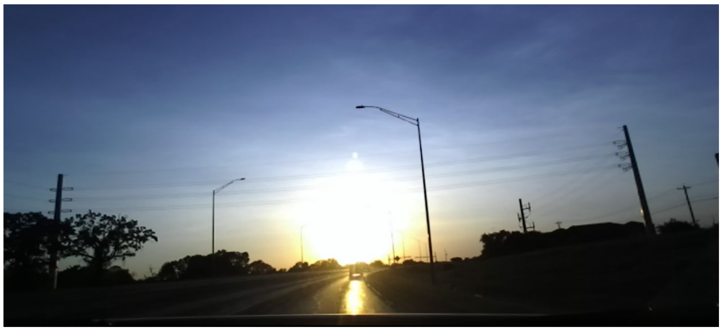
:1. Introduction
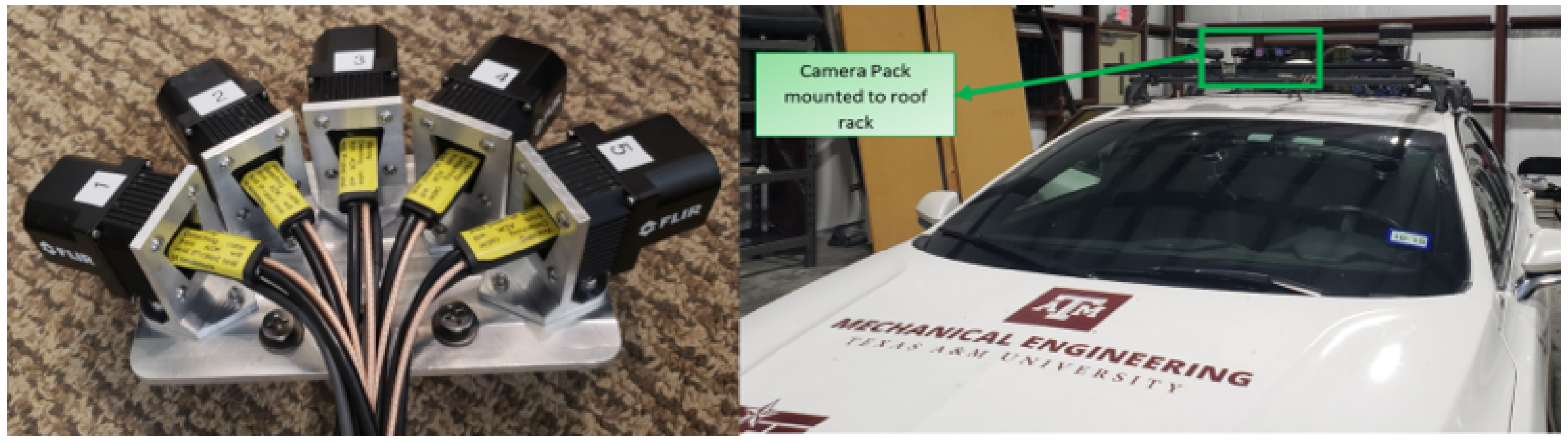
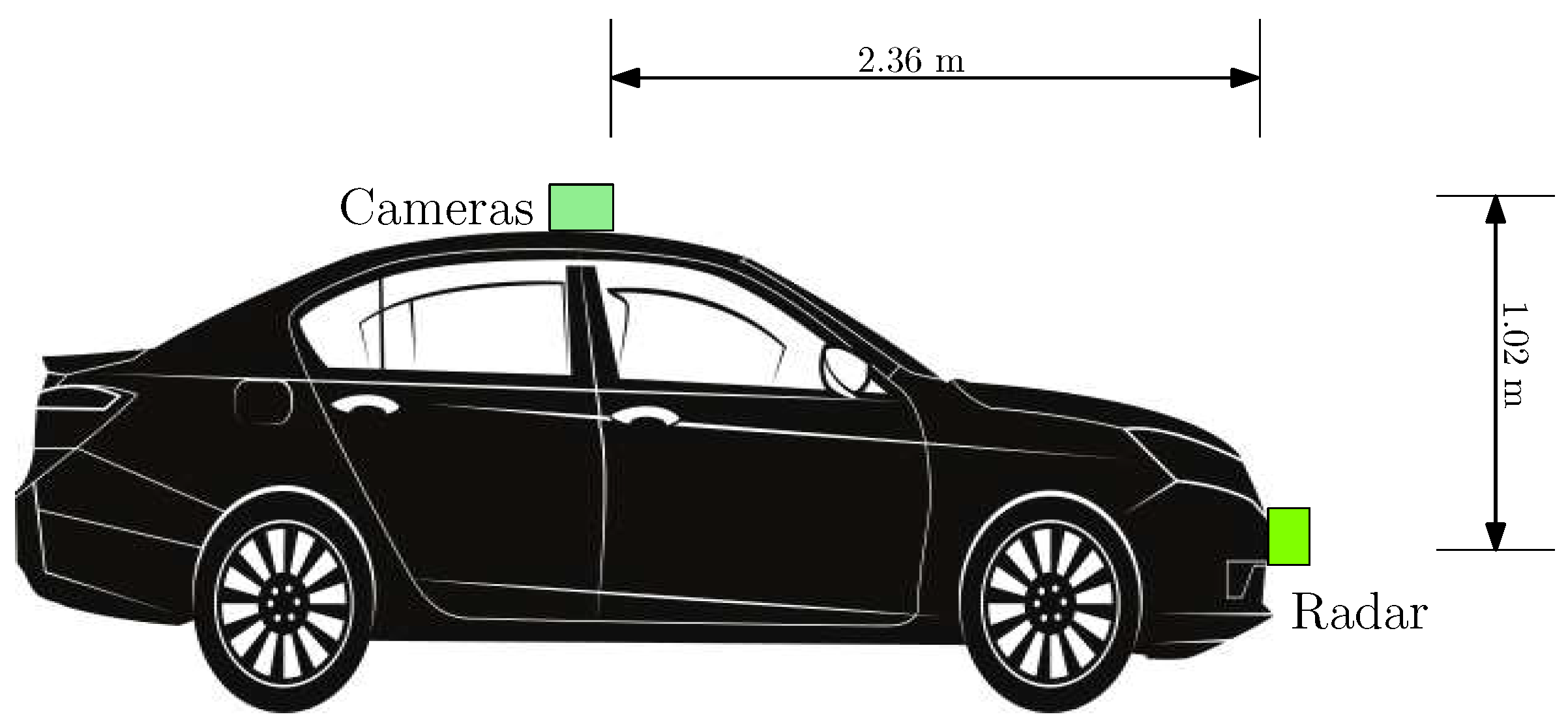
2. Sensor Configuration and Data Acquisition
2.1. Hardware
2.2. Software
- The width and height parameters of the network were changed to 1280 and 256, respectively. This would enable better detection of the 5:1 aspect ratio of the stitched video streams from the thermal camera assembly.
- The number of channels was changed from 3 (Red, Green, Blue) to 1 since the thermal cameras only output gray scale pixel information.
- The saturation and hue parameters were eliminated since these are only applicable for visible spectrum data.
3. Methodology: Sensor Fusion Multiple Object Tracking
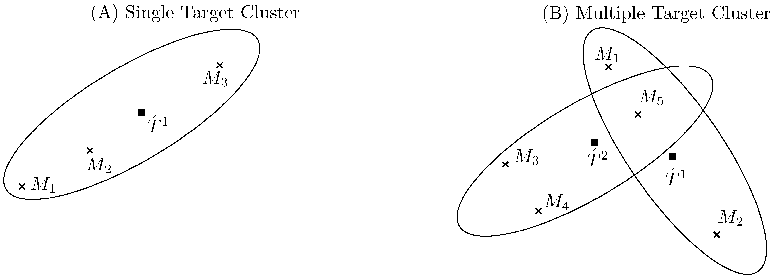
3.1. Model Assumptions
3.2. Track Initiation
3.3. Validation Gates and Track Maintenance
3.3.1. Joint Probabilistic Data Association
3.3.2. Multiple Hypothesis Tracking
3.4. Track Destruction
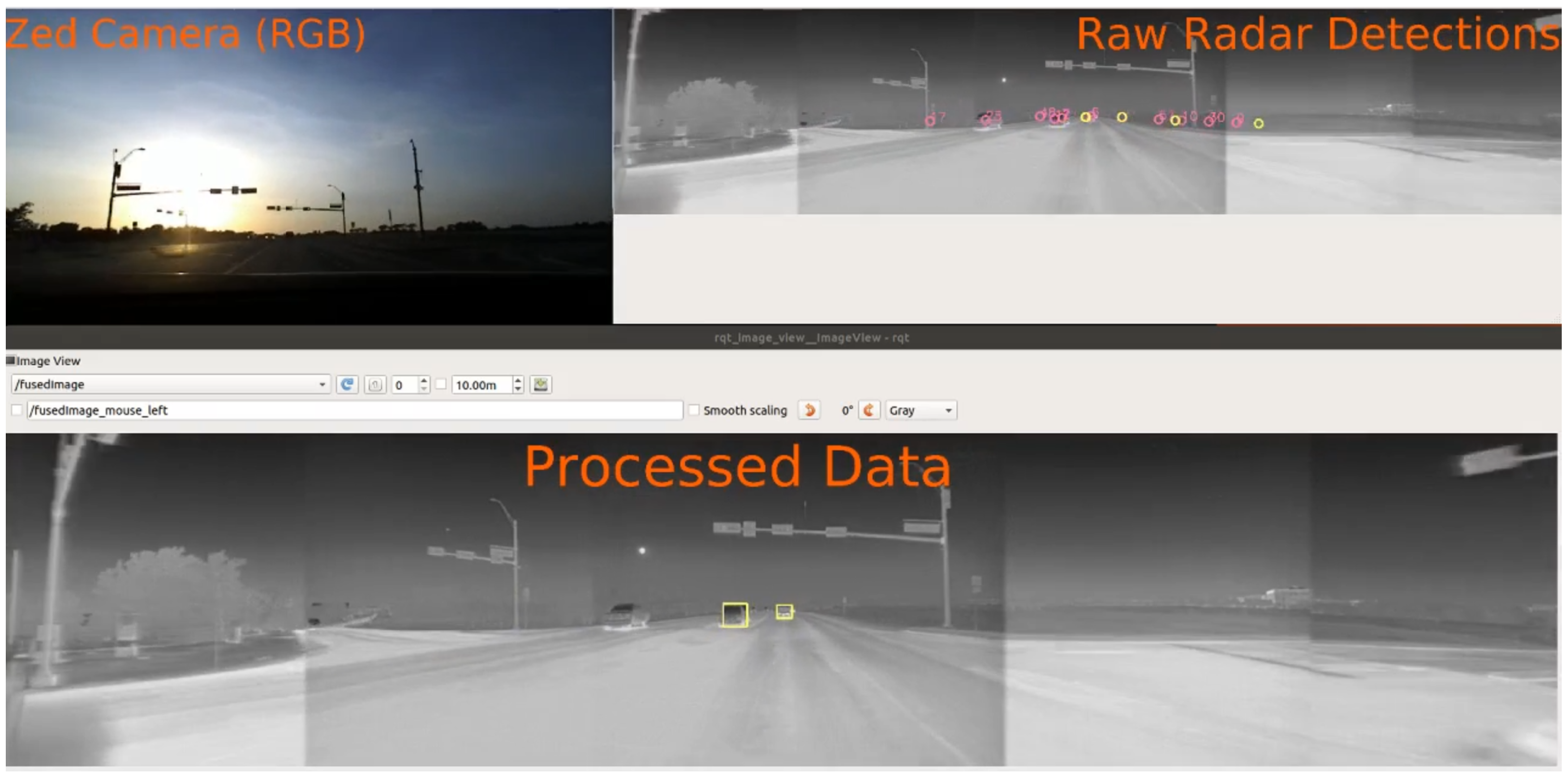
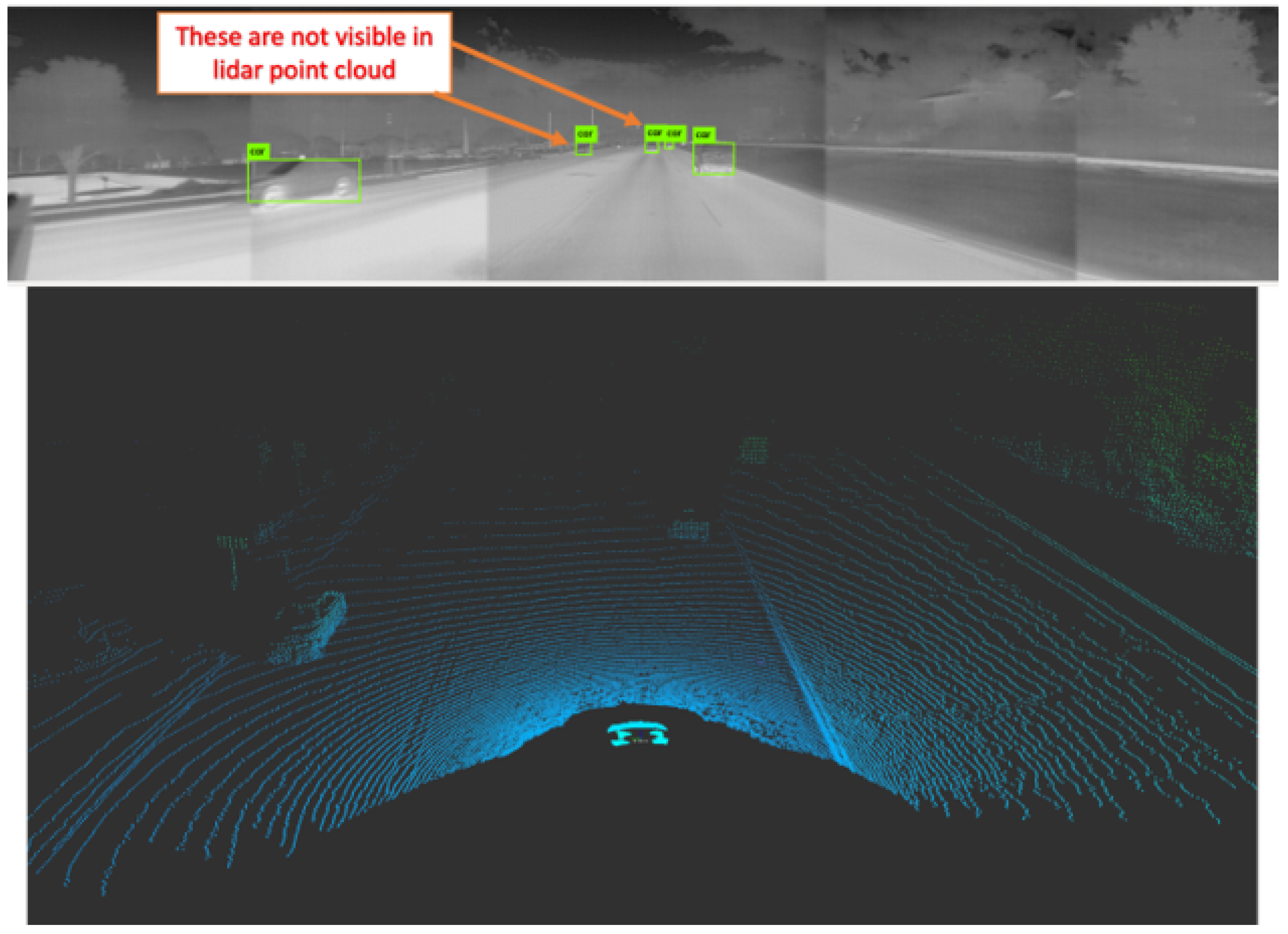
4. Results and Validation
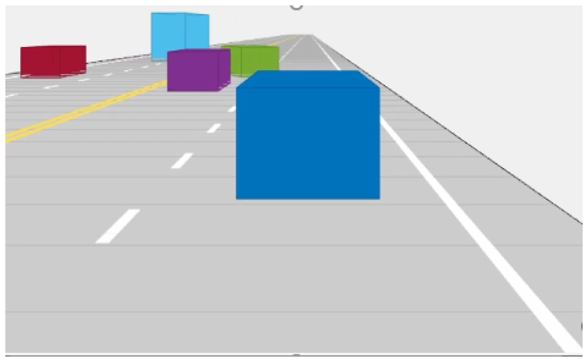
Quantifying the Performance Using a Digital Twin
5. Summary
Author Contributions
Funding
Institutional Review Board Statement
Informed Consent Statement
Data Availability Statement
Conflicts of Interest
Disclaimer
References
- Treat, J.R.; Tumbas, N.S.; McDonald, S.T.; Shinar, D.; Hume, R.D.; Mayer, R.E.; Stansifer, R.L.; Castellan, N.J. Tri-Level Study of the Causes of Traffic Accidents: Final Report. Volume I: Causal Factor Tabulations and Assessments; National Technical Information Service: Springfield, VA, USA, 1977; p. 609.
- National Highway Traffic Safety Administration. National Motor Vehicle Crash Causation Survey: Report to Congress: DOT HS 811 059; Createspace Independent Pub.: Scotts Valley, CA, USA, 2013. [Google Scholar]
- Sun, S.; Petropulu, A.P.; Poor, H.V. MIMO Radar for Advanced Driver-Assistance Systems and Autonomous Driving: Advantages and Challenges. IEEE Signal Process. Mag. 2020, 37, 98–117. [Google Scholar] [CrossRef]
- Gao, H.; Cheng, B.; Wang, J.; Li, K.; Zhao, J.; Li, D. Object Classification Using CNN-Based Fusion of Vision and LIDAR in Autonomous Vehicle Environment. IEEE Trans. Ind. Inform. 2018, 14, 4224–4231. [Google Scholar] [CrossRef]
- Prokhorov, D. A Convolutional Learning System for Object Classification in 3-D Lidar Data. IEEE Trans. Neural Netw. 2010, 21, 858–863. [Google Scholar] [CrossRef]
- SAE. Taxonomy and Definitions for Terms Related to On-Road Motor Vehicle Automated Driving Systems; SAE: Warrendale, PA, USA, 2014. [Google Scholar]
- Schoettle, B. Sensor Fusion: A Comparison of Sensing Capabilities of Human Drivers and Highly Automated Vehicles; Technical Report; University of Michigan Transportation Research Institute: Ann Arbor, MI, USA, 2017. [Google Scholar]
- Kutila, M.; Pyykönen, P.; Holzhüter, H.; Colomb, M.; Duthon, P. Automotive LiDAR performance verification in fog and rain. In Proceedings of the 2018 21st International Conference on Intelligent Transportation Systems (ITSC), Maui, HI, USA, 4–7 November 2018; pp. 1695–1701. [Google Scholar]
- Poland, K.; McKay, M.; Bruce, D.; Becic, E. Fatal crash between a car operating with automated control systems and a tractor-semitrailer truck. Traffic Inj. Prev. 2018, 19, S153–S156. [Google Scholar] [CrossRef] [PubMed]
- Paul, N.; Chung, C. Application of HDR algorithms to solve direct sunlight problems when autonomous vehicles using machine vision systems are driving into sun. Comput. Ind. 2018, 98, 192–196. [Google Scholar] [CrossRef]
- Bhadoriya, A.S.; Vegamoor, V.K.; Rathinam, S. Object Detection and Tracking for Autonomous Vehicles in Adverse Weather Conditions; SAE WCX Digital Summit; SAE International: Warrendale, PA, USA, 2021. [Google Scholar] [CrossRef]
- Davis, J.W.; Keck, M.A. A Two-Stage Template Approach to Person Detection in Thermal Imagery. In Proceedings of the 2005 Seventh IEEE Workshops on Applications of Computer Vision (WACV/MOTION’05)—Volume 1, Breckenridge, CO, USA, 5–7 January 2005; Volume 1, pp. 364–369. [Google Scholar] [CrossRef]
- Judd, K.M.; Thornton, M.P.; Richards, A.A. Automotive sensing: Assessing the impact of fog on LWIR, MWIR, SWIR, visible, and lidar performance. In Infrared Technology and Applications XLV; Andresen, B.F., Fulop, G.F., Hanson, C.M., Eds.; International Society for Optics and Photonics, SPIE: Bellingham, WA, USA, 2019; Volume 11002, pp. 322–334. [Google Scholar] [CrossRef]
- Forslund, D.; Bjärkefur, J. Night vision animal detection. In Proceedings of the 2014 IEEE Intelligent Vehicles Symposium Proceedings, Dearborn, MI, USA, 8–11 June 2014; pp. 737–742. [Google Scholar] [CrossRef]
- Kristoffersen, M.S.; Dueholm, J.V.; Gade, R.; Moeslund, T.B. Pedestrian Counting with Occlusion Handling Using Stereo Thermal Cameras. Sensors 2016, 16, 62. [Google Scholar] [CrossRef] [PubMed] [Green Version]
- Hwang, A. A Vehicle Tracking System Using Thermal and Lidar Data. Master’s Thesis, Texas A&M University, College Station, TX, USA, 2020. [Google Scholar]
- Choi, J.D.; Kim, M.Y. A Sensor Fusion System with Thermal Infrared Camera and LiDAR for Autonomous Vehicles and Deep Learning Based Object Detection. ICT Express 2022, in press. [CrossRef]
- Singh, A.; Vegamoor, V.K.; Rathinam, S. Thermal, Lidar and Radar Data for Sensor Fusion in Adverse Visibility Conditions (04-117). 2022. Available online: https://trid.trb.org/view/1925916 (accessed on 16 June 2021).
- Quigley, M.; Gerkey, B.; Conley, K.; Faust, J.; Foote, T.; Leibs, J.; Berger, E.; Wheeler, R.; Ng, A. ROS: An open-source Robot Operating System. In Proceedings of the IEEE International Conference on Robotics and Automation (ICRA) Workshop on Open Source Robotics, Kobe, Japan, 12–17 May 2009. [Google Scholar]
- Redmon, J.; Farhadi, A. YOLOv3: An Incremental Improvement. arXiv 2018, arXiv:cs.CV/1804.02767. [Google Scholar]
- FLIR. Thermal Dataset for Algorithm Training; FLIR Systems Inc.: Wilsonville, OR, USA, 2019. [Google Scholar]
- Bar-Shalom, Y.; Tse, E. Tracking in a Cluttered Environment With Probabilistic Data Association. Automatica 1975, 11, 451–460. [Google Scholar] [CrossRef]
- Morefield, C. Application of 0–1 Integer Programming to Multitarget tracking problems. IEEE Trans. Autom. Control 1977, 22, 302–312. [Google Scholar] [CrossRef]
- Reid, D.B. An Algorithm for Tracking Multiple Targets. IEEE Trans. Autom. Control 1979, 24, 843–854. [Google Scholar] [CrossRef]
- McMillan, J.C.; Lim, S.S. Data Association Algorithms for Multiple Target Tracking (U); Defense Research Establishment Ottawa: Ottawa, ON, Canada, 1990. [Google Scholar]
- Munkres, J. Algorithms for the Assignment and Transportation Problems. J. Soc. Ind. Appl. Math. 1957, 5, 32–38. [Google Scholar] [CrossRef] [Green Version]
- Fortmann, T.E.; Scheff, M.; Bar-Shalom, Y. Multi-Target Tracking using Joint Probabilistic Data Association. In Proceedings of the 1980 19th IEEE Conference on Decision and Control including the Symposium on Adaptive Processes, Albuquerque, NM, USA, 10–12 December 1980. [Google Scholar]
- Blackman, S. Multiple Hypothesis Tracking For Multiple Target Tracking. IEEE Aerosp. Electron. Syst. Mag. 2004, 19, 5–18. [Google Scholar] [CrossRef]
- Llinas, J.; Liggins, M.E.; Hall, D.L. Hand Book of Multisensor Data Fusion: Theory and Practice; CRC Press: Boca Raton, FL, USA, 2009. [Google Scholar]
- Pham, N.T.; Huang, W.; Ong, S.H. Probability Hypothesis Density Approach for Multi-camera Multi-object Tracking. In Computer Vision—ACCV 2007; Yagi, Y., Kang, S.B., Kweon, I.S., Zha, H., Eds.; Springer: Berlin/Heidelberg, Germany, 2007; pp. 875–884. [Google Scholar]
- Liu, M.; Rathinam, S.; Lukuc, M.; Gopalswamy, S. Fusing Radar and Vision Data for Cut-In Vehicle Identification in Platooning Applications. In WCX SAE World Congress Experience; SAE International: Warrendale, PA, USA, 2020. [Google Scholar] [CrossRef]
- Bar-Shalom, Y. Multitarget-Multisensor Tracking Principles and Techniques; YBS Publishing: Storrs, CT, USA, 1995. [Google Scholar]
- Fisher, J.L.; Casasent, D.P. Fast JPDA multitarget tracking algorithm. Appl. Opt. 1989, 28, 371. [Google Scholar] [CrossRef] [PubMed]
- Zhou, B.; Bose, N.K. Multitarget Tracking in Clutter: Fast Algorithms for Data Association. IEEE Trans. Aerosp. Electron. Syst. 1993, 29, 352–363. [Google Scholar] [CrossRef]
- Sittler, R.W. An Optimal Data Association Problem in Surveillance Theory. IEEE Trans. Mil. Electron. 1964, 8, 125–139. [Google Scholar] [CrossRef]
- Whitley, J. ROS Driver for the FLIR Boson USB Camera. 2019. Available online: https://github.com/astuff/flir_boson_usb (accessed on 14 June 2022).
- Stanislas, L.; Peynot, T. Characterisation of the Delphi Electronically Scanning Radar for robotics applications. In Proceedings of the Australasian Conference on Robotics and Automation 2015, Canberra, Australia, 2–4 December 2015. [Google Scholar]


| Measurements per Cluster | Number of Targets | |||
|---|---|---|---|---|
| 1 | 2 | 5 | 10 | |
| 1 | 2 | 3 | 6 | 11 |
| 2 | 3 | 7 | 31 | 111 |
| 5 | 6 | 31 | 1546 | 63,591 |
| 10 | 11 | 111 | 63,591 | 2.34 × 10⁸ |
| Identification Recall (IDR) | Identification Precision (IDP) | |
|---|---|---|
| JPDA | ||
| MHT |
Publisher’s Note: MDPI stays neutral with regard to jurisdictional claims in published maps and institutional affiliations. |
© 2022 by the authors. Licensee MDPI, Basel, Switzerland. This article is an open access article distributed under the terms and conditions of the Creative Commons Attribution (CC BY) license (https://creativecommons.org/licenses/by/4.0/).
Share and Cite
Bhadoriya, A.S.; Vegamoor, V.; Rathinam, S. Vehicle Detection and Tracking Using Thermal Cameras in Adverse Visibility Conditions. Sensors 2022, 22, 4567. https://doi.org/10.3390/s22124567
Bhadoriya AS, Vegamoor V, Rathinam S. Vehicle Detection and Tracking Using Thermal Cameras in Adverse Visibility Conditions. Sensors. 2022; 22(12):4567. https://doi.org/10.3390/s22124567
Chicago/Turabian StyleBhadoriya, Abhay Singh, Vamsi Vegamoor, and Sivakumar Rathinam. 2022. "Vehicle Detection and Tracking Using Thermal Cameras in Adverse Visibility Conditions" Sensors 22, no. 12: 4567. https://doi.org/10.3390/s22124567
APA StyleBhadoriya, A. S., Vegamoor, V., & Rathinam, S. (2022). Vehicle Detection and Tracking Using Thermal Cameras in Adverse Visibility Conditions. Sensors, 22(12), 4567. https://doi.org/10.3390/s22124567