1. Introduction
With the rapid development of control and network technology, unmanned aerial vehicles (UAV) have been a prominent research topic in both academic and engineering fields in recent years. A variety of application scenarios have been employed by UAVs, such as search and rescue [
1,
2,
3], express transportation [
4,
5], and remote sensing [
6]. Furthermore, it is worth mentioning that multiple UAVs can accomplish complex tasks with more robustness and efficient working ability than a single UAV. As one of the interesting control issues, the formation problem for UAVs has gained significant research attention [
7,
8,
9,
10]. Specifically, the communication topology for UAVs has played a key role since all the information exchanges are achieved via the communication network. It should be pointed out that it is always difficult or expensive to hold fixed communication topology within different task assignments or in an unstructured environment with disturbances. Furthermore, the varying topology may exhibit certain random features in some conditions. Hence, it is natural and important to investigate the formation protocol with random topologies [
11,
12,
13]. On the other hand, lots of studies have shown that the Markov process could be adopted to describe these stochastic jumping features between different modes accurately. As a result, some initial efforts have been made toward Markovian jumping communication topologies. However, notice that the transition probabilities of a Markovian jumping system are conformed to be a fixed exponential distribution, which would lead to certain restrictions in practical applications. In fact, time-varying transition probabilities are more general in implementations, and the semi-Markov process is able to depict these time-varying transition probabilities [
14,
15,
16,
17]. As far as the authors’ knowledge extends, there is still huge room for studies on the integration of semi-Markovian jumping topology and UAV formation problems.
Another active research field is networked control systems, where the event-triggered schemes have aroused great concern recently [
18,
19,
20]. As we well know, computational and network resources are very valuable for UAVs. Under this context, the event-triggered communication schemes could considerably improve communication efficiency and optimize data transmission compared to traditional time-triggered ones [
21,
22,
23]. Moreover, when taking into account the topology jumpings, the vast majority of event-triggered schemes do not utilize mode information well, and thus, the acquired results are conservative in certain senses. It is noteworthy that control strategies for Markov/semi-Markov jumping systems could utilize the involved information on active modes to improve control effects substantially. In short, the mode-dependent event-triggered strategies are more applicable in practical applications [
14,
24]. However, it is necessary to point out the fact that constructing an available mode-dependent triggering scheme by events is difficult and challenging. To date, to the best of our knowledge, there are few results on the formation of UAVs with semi-Markovian jumping topology. This motivates us to shorten this gap.
In light of the aforementioned discussions, our aim is to explore the mode-dependent event-triggered strategy for UAVs formation problems with semi-Markovian jumping topology within a finite-time framework. More precisely, the concept of finite-time passivity is employed for disturbance attenuation during UAV formation while the transient performance of formation dynamics is achieved. Compared with most reporting works, the novelties of our paper are threefold. First, the finite-time formation model of UAVs is formulated with sufficient consideration of semi-Markovian jumping topologies. Secondly, an original asynchronous mode-dependent event-triggering strategy is developed for UAVs in order to improve the communication efficiency through reducing data transmissions. Thirdly, according to model transformation and the Lyapunov–Krasovskii functional, a distributed formation protocol has been developed to satisfy the finite-time passivity performance in the mean-square sense.
The rest of our work is as listed following. In
Section 2, we construct the formation model of UAVs with regard to semi-Markovian jumping topologies and design the asynchronous mode-dependent event-triggering formation protocol. Then, sufficient conditions satisfying finite-time passivity performance would be verified and given with reliable details in
Section 3. After that, the simulation results are illustrated with numerical simulations in
Section 4 to verify the correctness of our derived designs. Finally, the conclusion and expectation of this paper are given in
Section 5.
The notations in this paper are given in
Table 1.
2. Problem Formulation
Given a probability space
and denote
as a continuous-time discrete-state semi-Markov process, which takes values in a finite set
. The transition probability matrix
,
,
is defined as follows
Accordingly, we introduce a directed graph
to depict the communication topology among the UAVs.
and
represent for the sets of nodes and edges,
represents the weighted adjacency matrix by
respectively. Moreover, the Laplacian matrix of
is defined by
with
By employing the graph theory, one can verify for any possible
and a full row rank matrix
[
25]
there must exist a matrix
satisfying
.
For the formation of UAVs, a typical outer/inner-loop design structure is utilized [
26]. Then, consider the group of
N quadrotors with double integrator dynamics described as follows:
where
,
and
represent the position, velocity and formation control input vector, respectively.
Remark 1. The notable outer/inner-loop formation control configuration for quadrotors has been widely studied, where the outer-loop control is devoted to the desired position and velocity of UAVs. Under this context, the double integrator point-mass model can be effectively adopted to describe the formation dynamics of UAVs.
By taking into account the external disturbances, the following state-space model of each UAV can be rewritten by:
where
,
denotes the formation control input,
represents the external disturbances and
Suppose that all UAVs share a unified communication network with semi-Markovian jumping topologies. Accordingly, we assume that a mode-dependent sampling period
is adopted, such that local information exchanges are accomplished between neighboring UAVs. Furthermore, the following asynchronous mode-dependent event triggering communication strategy is applied
where
and
represents the latest
kth updating instant of the
mth UAV,
represents the triggering threshold,
and
represents the weighting matrices. It can be found that based on the proposed asynchronous event-triggered strategy, the information updates of the UAVs only require the neighboring information exchanges instead of the overall states of UAVs, which is more applicable for the distributed local communications of the UAVs. In conclusion, detailed notations of these parameters are given in the following
Table 2.
In the sequel, the formation configuration definition is given as follows:
Definition 1. The distributed formation configuration can be accomplished if it holds thatwhere represents the relative formation configuration distance. Denote
, and design the formation control input by
where
represents the mode-dependent gains to be determined. As a result, by letting
and dividing
into
intervals, it yields that
Based on the above results, one can further obtain that
where
Note that the resulting closed-loop dynamics can be rewritten as follows:
where
For simplicity of description, denote
and one has
Recalling that
, it can be obtained that
where
represents the formation error of
and
,
, respectively.
Before proceeding, the following definitions are given for the transient performance of formation dynamics [
27,
28].
Definition 2. Given constants , , , and matrix , the finite-time boundedness formation is achieved with respect to in a mean-square sense, if it holds that Definition 3. Given constants , , , , and matrix , the finite-time passivity formation is achieved with respect to in mean-square sense, if finite-time boundedness is satisfied and it holds that Remark 2. It should be pointed out that based on model transformation, the finite-time formation control problem is converted to the finite-time stability (passivity performance) control problem. The concept of finite-time stability (passivity performance) of formation errors is then investigated, where the asymptotic behavior over a finite-time interval is concerned instead of infinite-time stability, which implies that the prescribed upper bound can be satisfied during the prescribed time intervals. The mean-square finite-time passivity performance not only focuses on the dynamical features within a finite time interval but also deals with the disturbances from an energy point of view. It should be pointed out that mean-square finite-time passivity may not be Lyapunov mean-square passivity and vice versa.
Hence, our main aim is to design the mode-dependent formation control gains
to guarantee finite-time passivity formation. The following matrix lemma can be provided to derive further results [
29].
Lemma 1. Given matrix , satisfying , , and such that it holds thatwhere 3. Main Results
This section gives the detailed formation controller design procedure with the aid of convex optimization and the matrix technique.
Theorem 1. For given , the finite-time formation problem of UAVs (3) can be solved with designed formation controller gains if there exist mode-dependent matrices , , , such that holds for all , whereandwith Proof. Construct mode-dependent Lyapunov–Krasovskii functionals as follows:
where
Moreover, we defined the weak infinitesimal operator for
by
with
where
represents the cumulative distribution function of the sojourn time, and
denotes the probability intensity.
By employing the input-delay strategy, one has
where
with
As a result, it can be derived that
Similarly, it can be obtained that
By employing Lemma 1 to
, one has
where
Meanwhile, the event-triggered function implies that
Then, we can derive the following matrix inequality
where
Hence, we can verify that when
in Theorem 1 holds, it satisfies that
where
Furthermore, it can be derived that
Consequently, we have that
where
This means that can be finite-time boundedness according to Definition 2, and we thus finish this proof. □
Theorem 2. For given , the finite-time formation problem of UAVs (3) can be solved, if there exist mode-dependent matrices , , and constant , such that , , and holds for all and , wherewith Proof. Following similar proofs in Theorem 1, it can be derived that
such that
can guarantee that the above matrix inequality holds, where
Consequently, it yields that
which holds with
that
with
Subsequently, by performing matrix congruent transformation to
with
and letting
one has
Meanwhile, by letting
with
one has
which leads to
and
. Moreover, it follows that
and
such that
and
. Then, we have
Finally, by adopting the method for the time-varying dwell time , , , , the remainder of the proof can follow conveniently from Theorem 1, which ensures that the finite-time passivity formation can be satisfied according to Definition 3. □
Remark 3. The computation complexity for the above linear matrix inequality (LMI) convex optimization conditions is related to the convex combination representation of time-varying dwell time with . As such, it is a trade-off to setting an appropriate ι for better describing the time-varying dwell time and computation complexity of LMIs.
4. Simulation Results
This section demonstrates the effectiveness of theoretical results via the numerical simulation results.
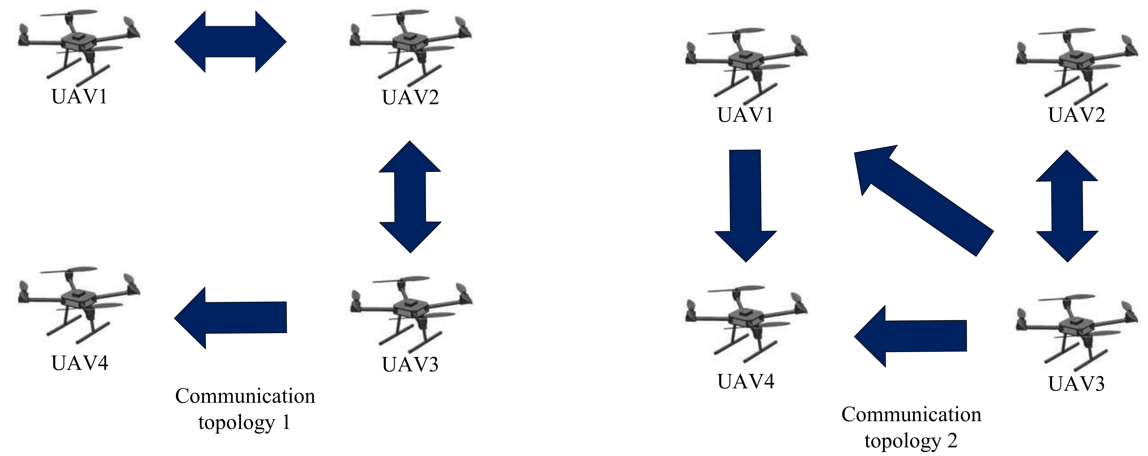
As depicted in
Figure 1, consider a group of four UAVs and the corresponding Laplacian matrices of communication topology are given by
with
The transition rates of semi-Markov topologies are assumed to be
and
. Accordingly, we can set
and it follows that
,
,
and
. The formation configuration is supposed to be
,
,
,
. For the event-triggered communication, the scalar parameters are set by
and
with
s and
s. In terms of Theorem 2 with finite-time passivity performance
, the values of mode-dependent formation controller gains and triggering matrices are achieved by solving the convex optimization problem as follows:
and
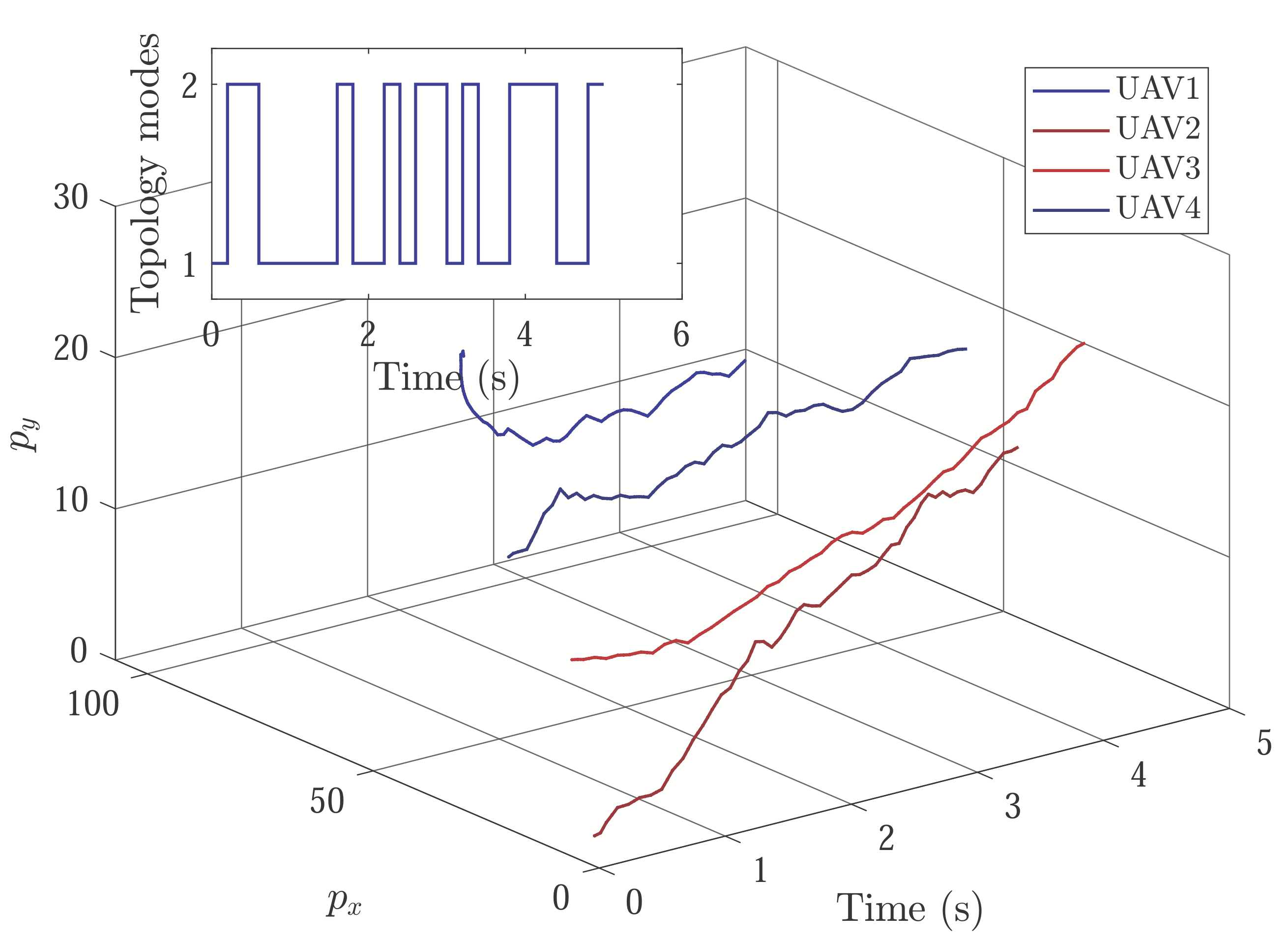
With initial conditions and setting
,
Figure 2 and
Figure 3 show the resulting formation trajectories of UAVs. More precisely, it can be observed that the UAVs can achieve converging motion within the prescribed finite time interval. Moreover, one can verify from
Figure 3 that the finite-time boundedness can be ensured with
and
by Definition 2.
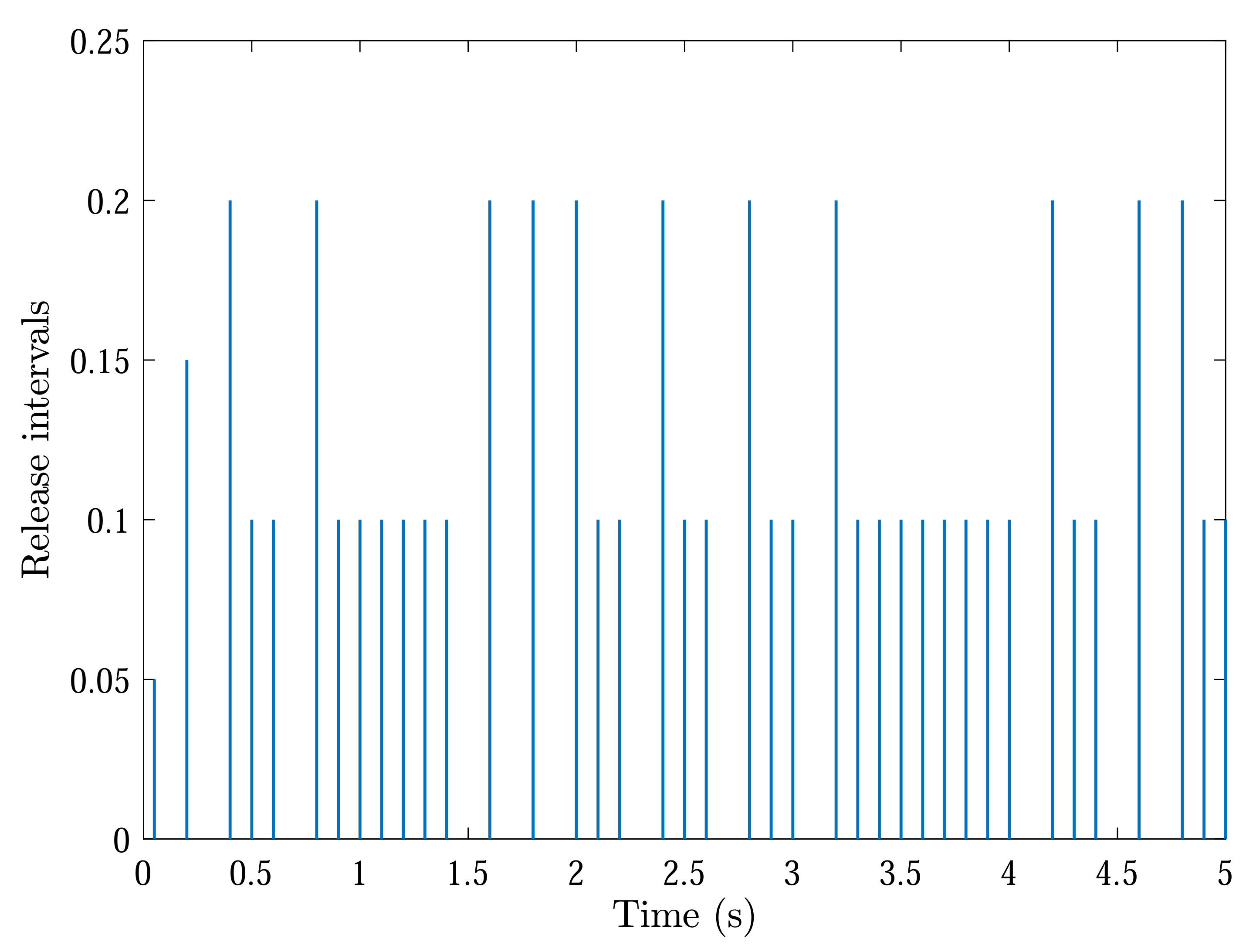
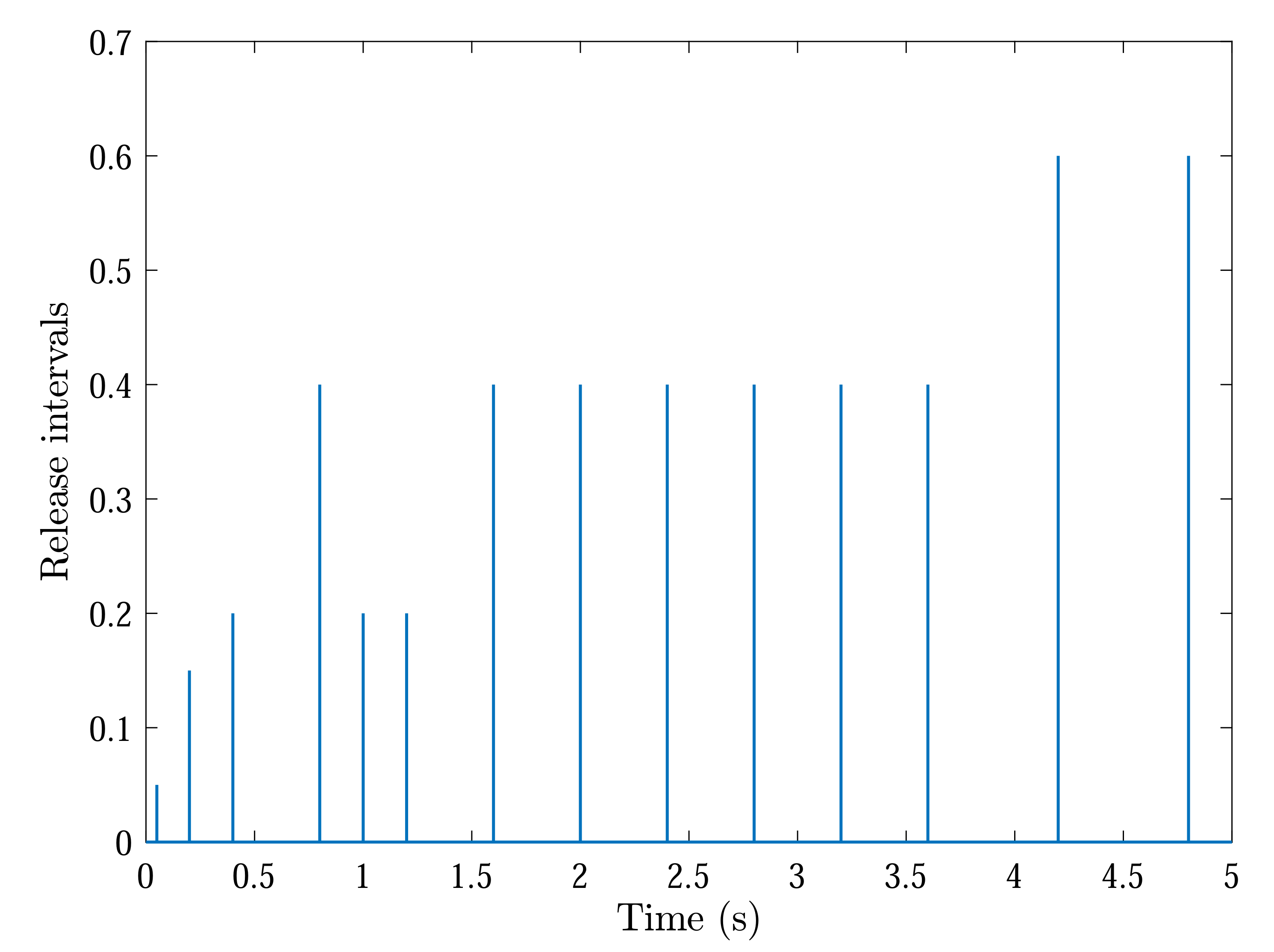
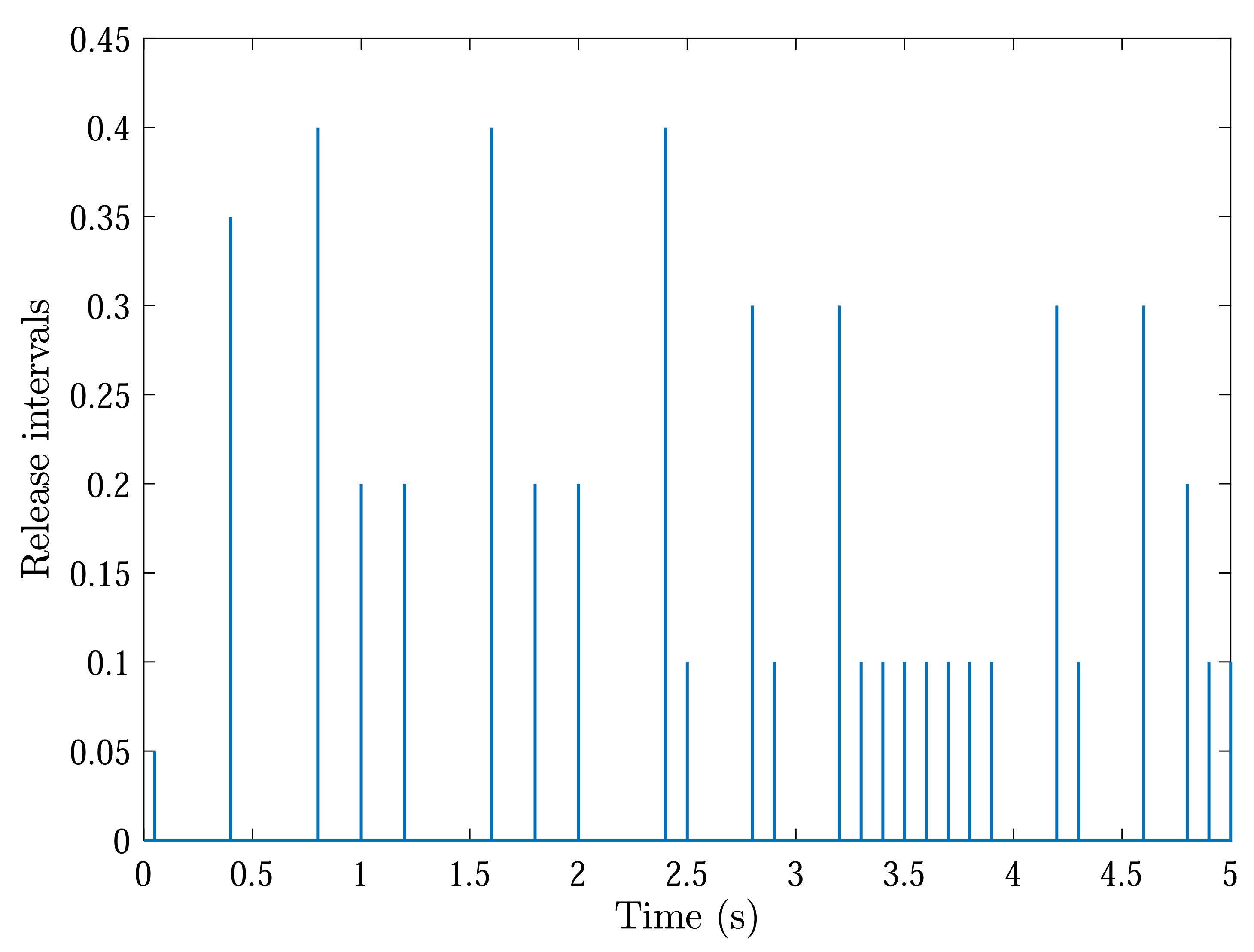
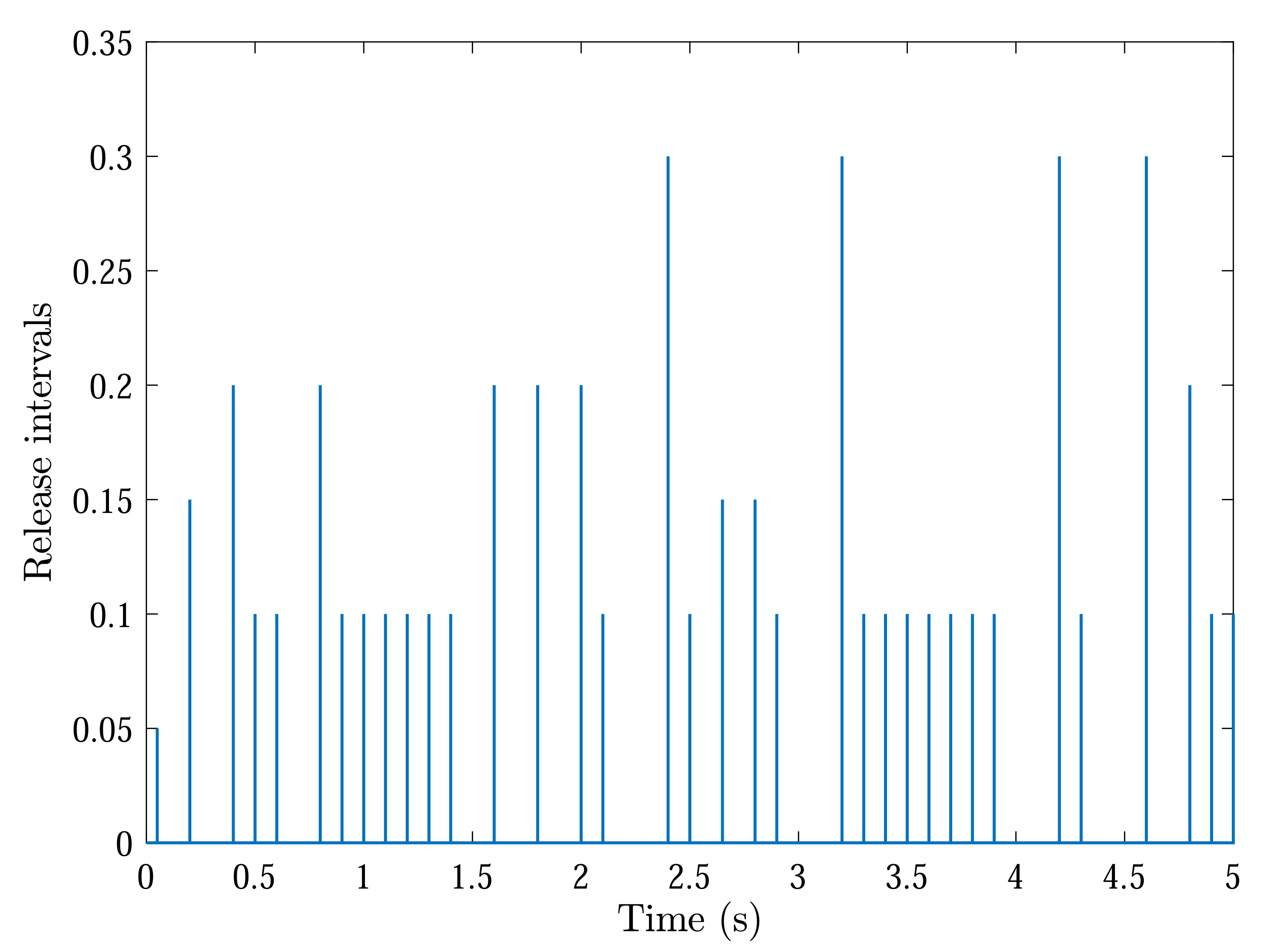
Figure 4,
Figure 5,
Figure 6 and
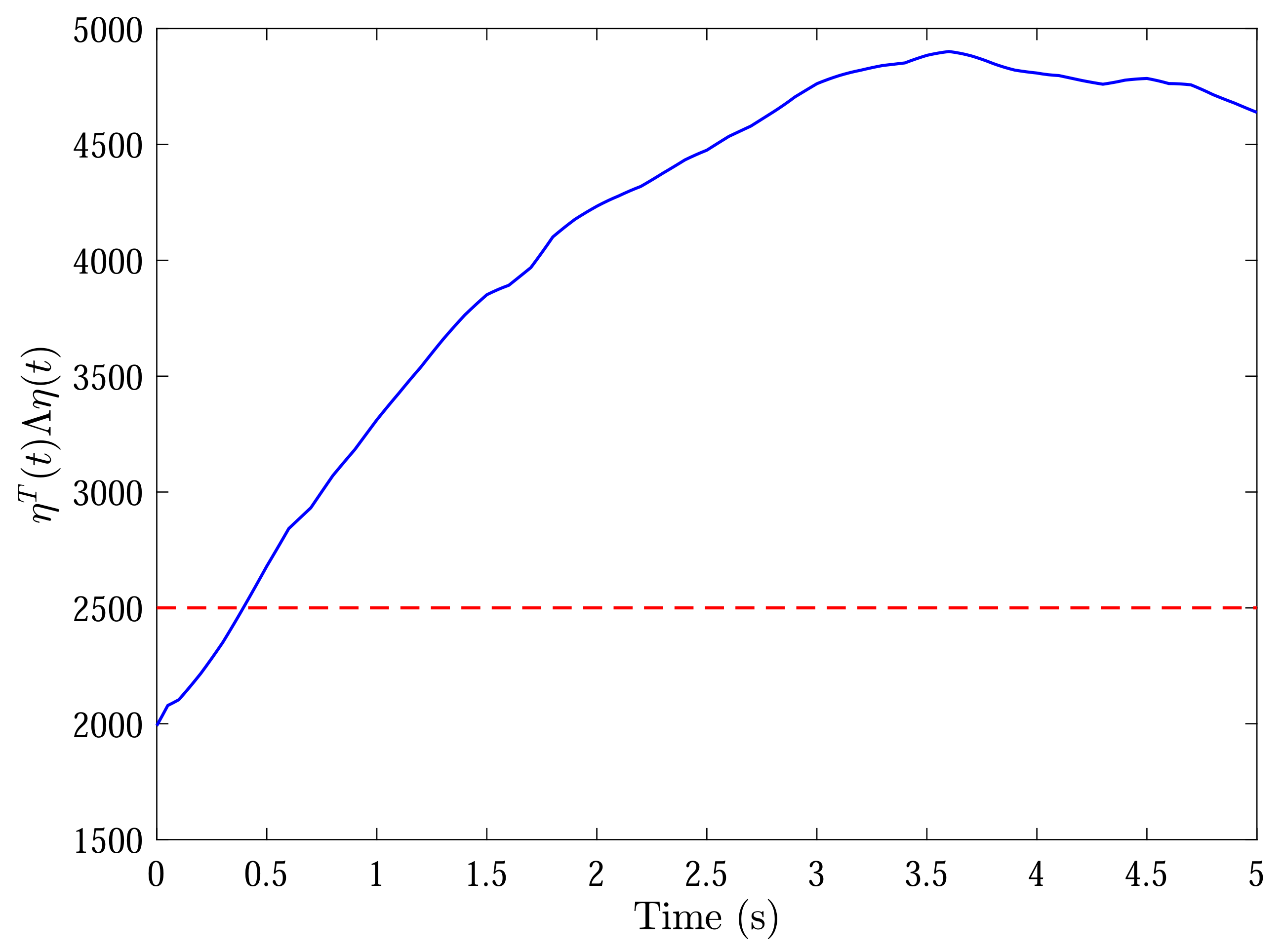
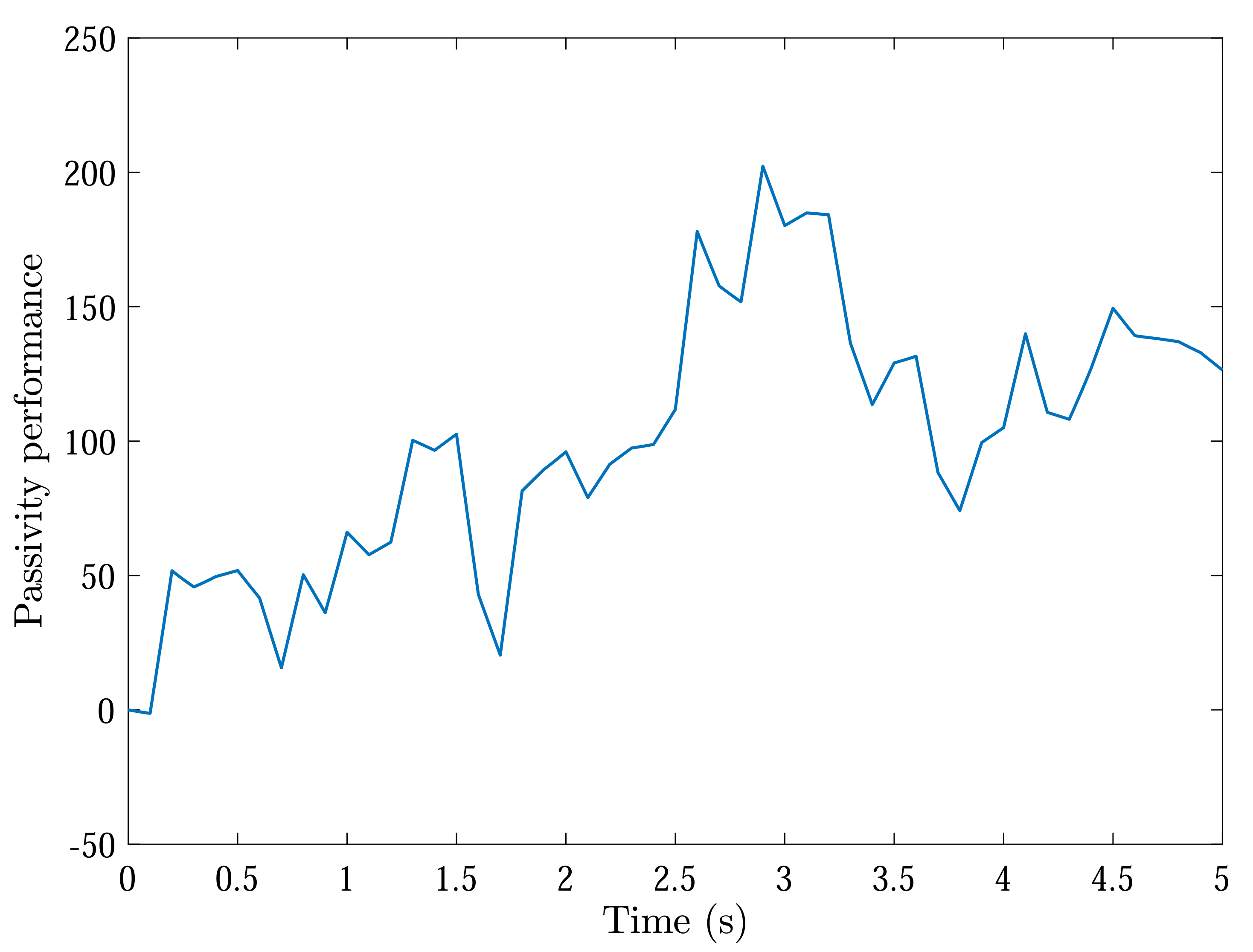
Figure 7 reveal the data broadcasting instants with release intervals of UAVs, from which one can find that the signal transmissions can be effectively decreased compared with the traditional time-triggered approaches, such that the local communication efficiency among the UAVs can be increased under the distributed formation control framework. Furthermore, it can be seen from
Figure 8 that the finite-time passivity condition can be satisfied according to Definition 3 with


