
Bridge Crack Inspection Efficiency of an Unmanned Aerial Vehicle System with a Laser Ranging Module


 , ,
, ,
Abstract
:1. Introduction
- (1)
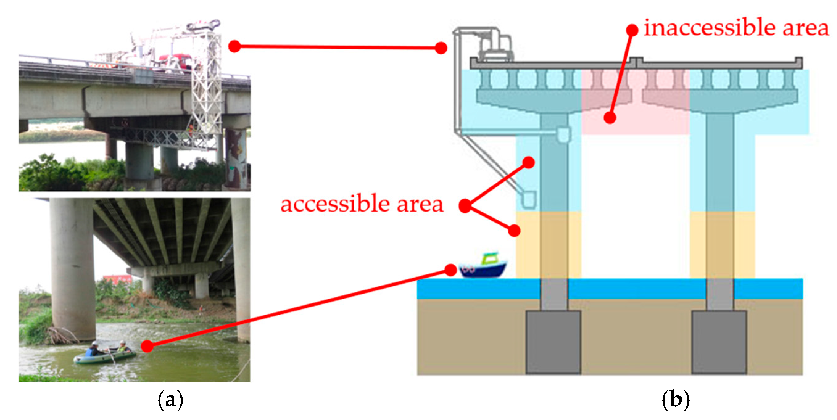
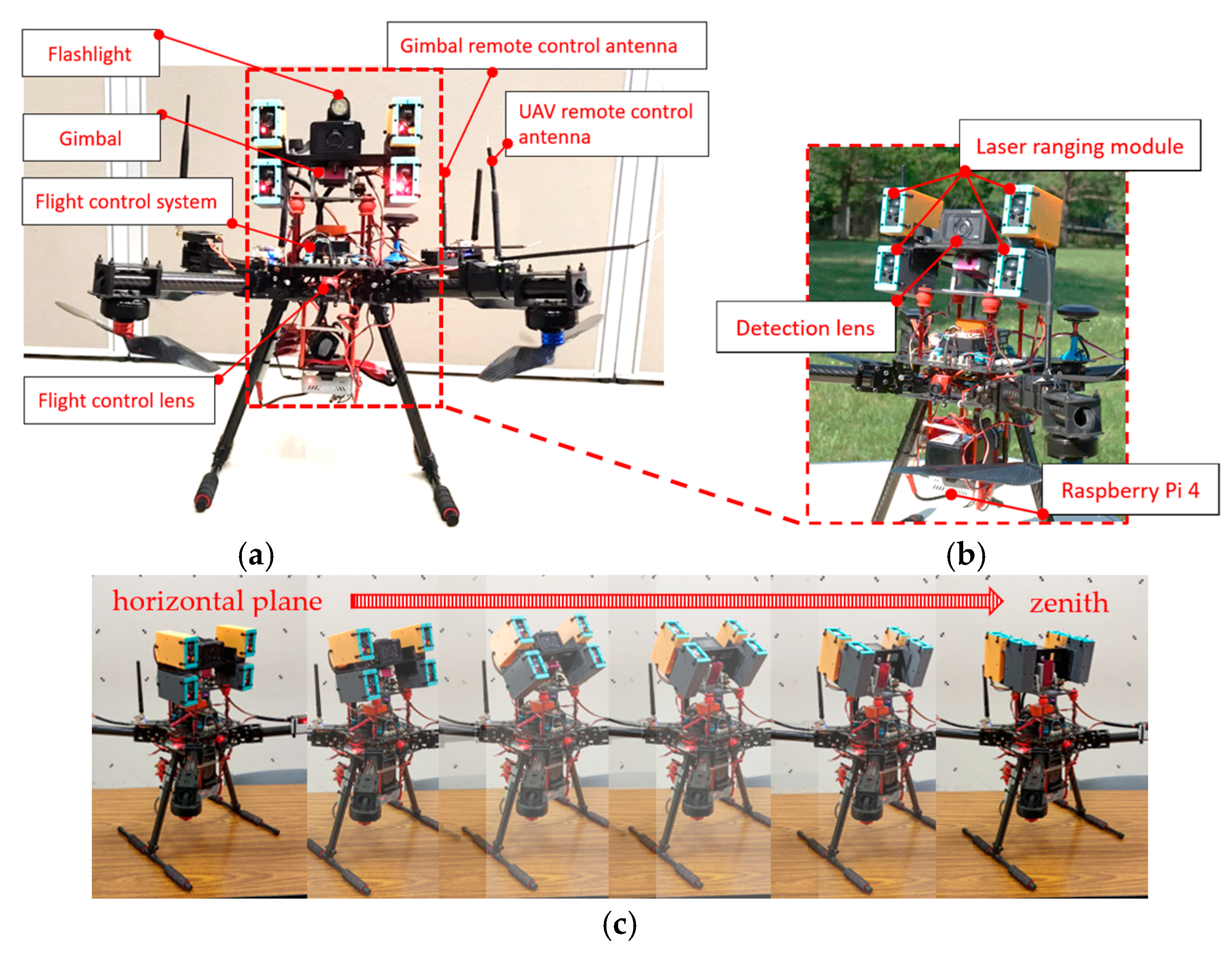
- This study developed an adapted UAV for bridge inspection operations and the inspection camera. The camera is installed on the tripod head and can rotate from 90° (horizontal plane) to 180° (zenith), which enables the UAV to inspect the sides and bottom of bridges.
- (2)
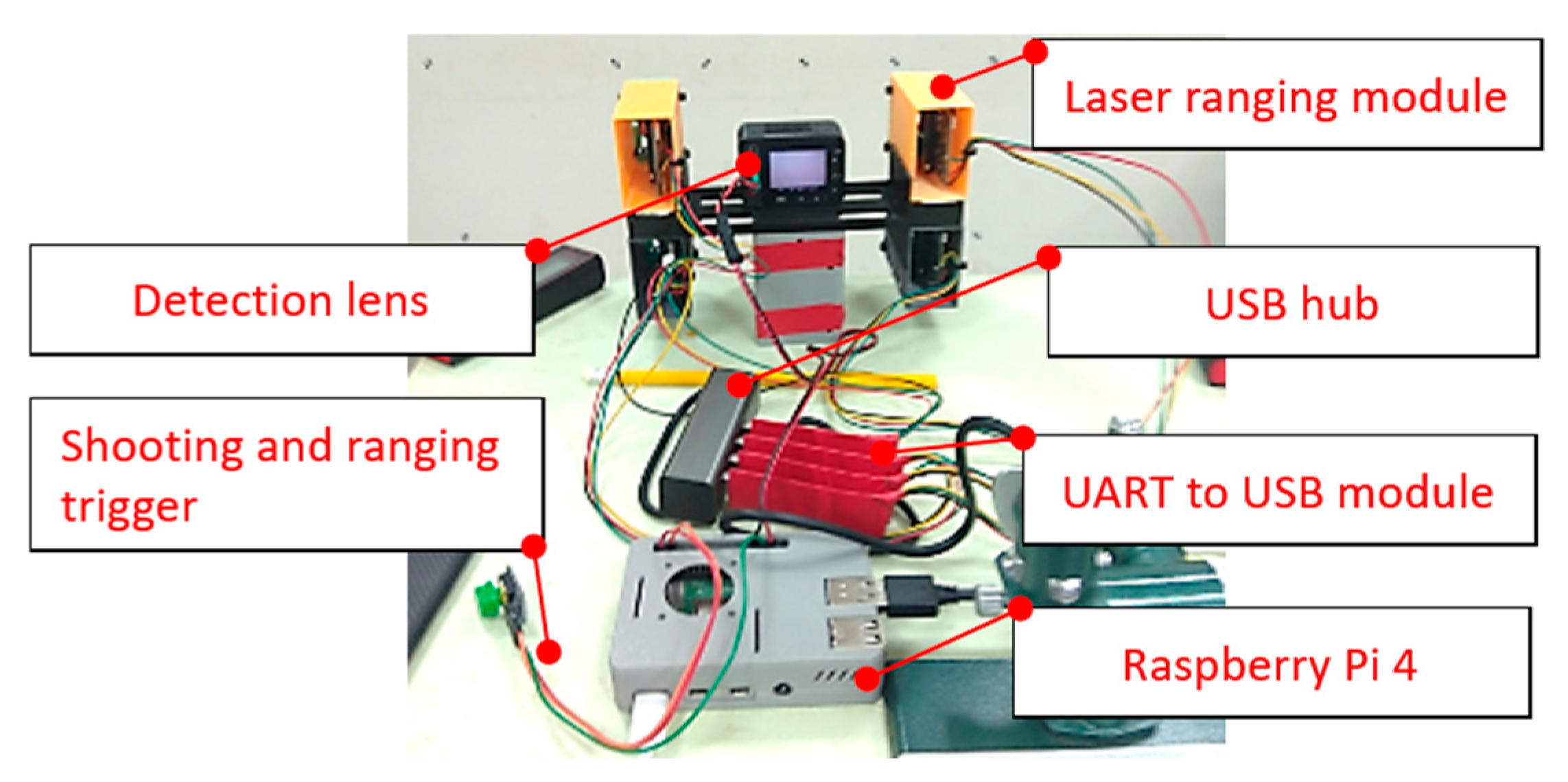
- This study developed the architecture and method used to integrate the camera and the laser ranging module on the embedded system (Raspberry Pi 4). Additionally, the object projection measurement method was proposed, which can overcome the limitations of vertical photography.
- (3)
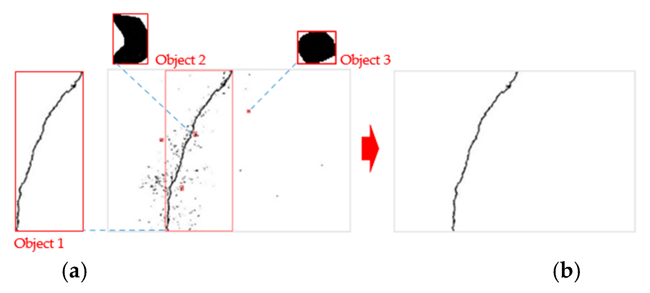
- This study proposed an image-processing method and process to extract crack information and metric size.
2. Materials and Methods
2.1. Design and Development of a UAV System for Bridge Inspection
2.2. Integration of the Camera and a Laser Ranging Module
2.2.1. Synchronization Mechanism for the Operation Time of the Camera and Laser Ranging Modules
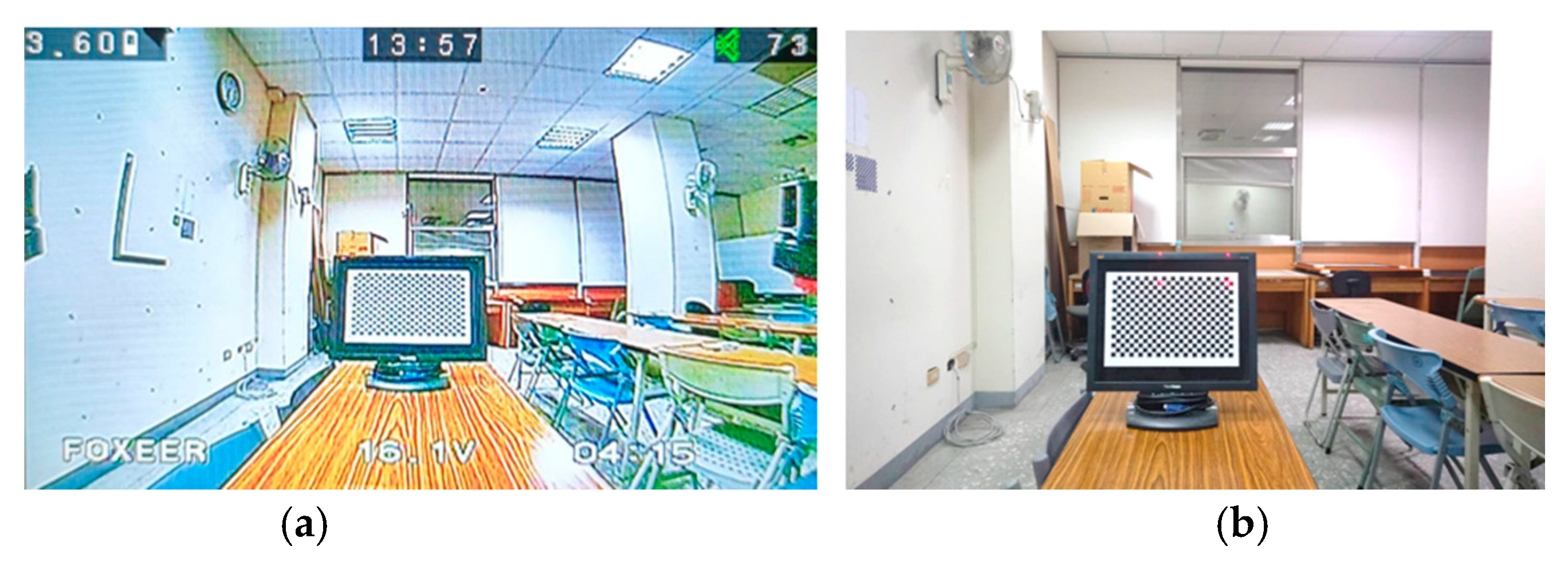
2.2.2. Camera Calibrations
2.2.3. Overall Structural Calibrations for the Camera and Laser Ranging Modules
- (1)
- The positions of the ranging modules were adjusted so that the four laser beams were nearly parallel to each other. Subsequently, the measurement accuracy was increased by measuring the laser beam vectors after calibration.
- (2)
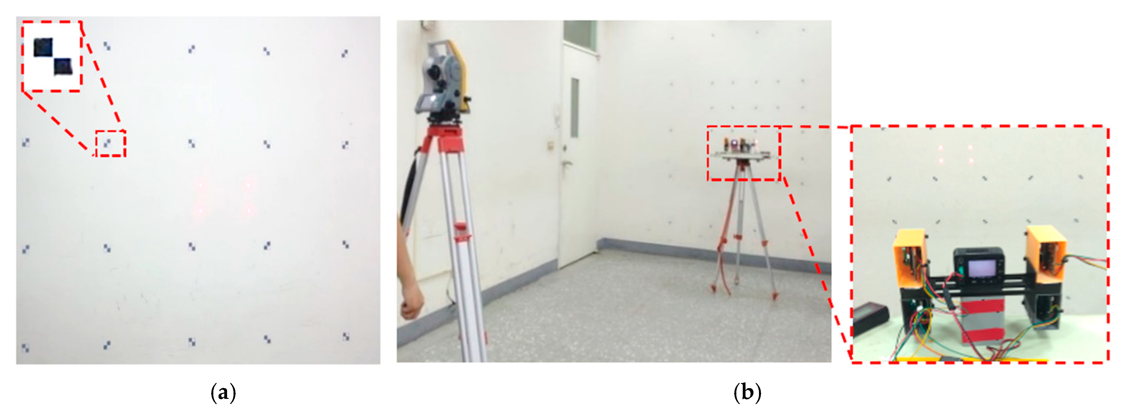
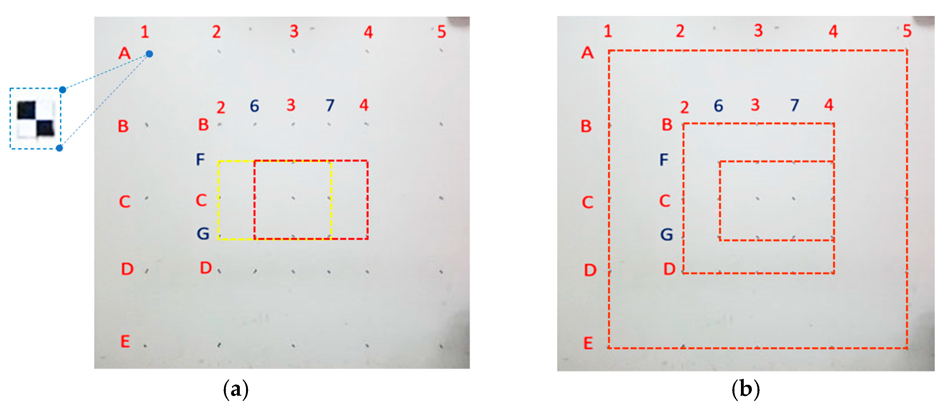
- As the spatial relationships between the laser beam vectors and the camera focus could not be directly measured, control points were marked on the wall of a research room, and relative spatial coordinates were measured using a total station. The room served as the system calibration site. Photos containing laser light spots and control points were captured from different distances (Figure 8a), and photogrammetry was used to calculate the spatial relationships between the laser beam vectors and the laser light spots, as well as those between the laser beam vectors and the control points. The experimental distance was increased from 1 to 3 m in 0.5-m increments. To demonstrate that the developed system can capture images with different attitudes, images were captured in five postures (i.e., facing forward, tilted to the left, tilted to the right, tilted up, and tilted down) in every test, and the ranging modules were used to measure distances. A total of 25 image sets and ranging data were collected, and the spatial coordinates of the laser light spots were simultaneously measured using the total station (Figure 8b).
- (3)
- As the camera was in different locations and at different attitudes when capturing different images, laser light spots could not be used to calculate the laser beam vectors. Thus, the control point coordinates of the photos and collinear spatial resections were used to calculate the outer orientation parameters of the images. The outer orientation was used as a basis to translate and rotate the coordinate system of each photo to a coordinate system in the same space. The converted laser light spots were subsequently used to calculate the laser beam vectors and laser launch point coordinates. The collinearity equations are as follows:where is the focal length of the camera, coordinates of the principle point of a photo, are photo coordinates of the corrected control point, are object spatial coordinates the camera projection center, are object spatial coordinates of the control point, are rotation matrices composed of the image spatial rotation angles.
2.2.4. Indoor Measurement Accuracy Tests for the Camera and Laser Ranging Modules
2.3. Crack Identification and Measurement Methods
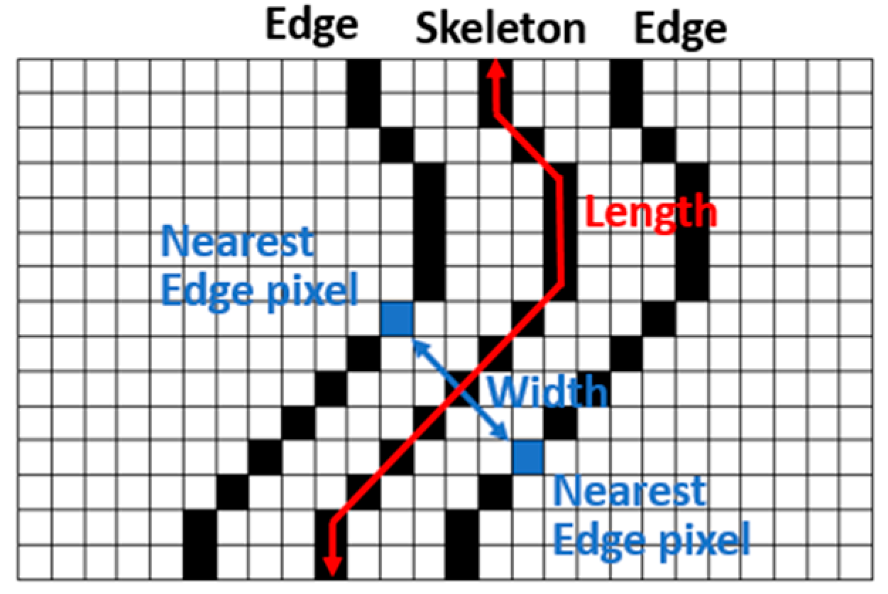
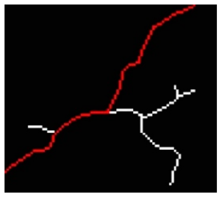
2.3.1. Extracting the Length of the Main Crack Skeleton
2.3.2. Extraction of Crack Widths
3. Crack Inspection Efficiency and Accuracy of the Developed UAV System
3.1. Outdoor Bridge Inspection Tests
3.2. Outdoor Bridge Inspection Tests
- (1)
- Case 1
- (2)
- Case 2
- (3)
- Case 3
4. Conclusions
Author Contributions
Funding
Institutional Review Board Statement
Informed Consent Statement
Data Availability Statement
Conflicts of Interest
References
- Hallermann, N.; Morgenthal, G. Visual inspection strategies for large bridges using Unmanned Aerial Vehicles (UAV). In Proceedings of the 7th International Conference on Bridge Maintenance, Safety and Management (IABMAS 2014), Shanghai, China, 7–11 July 2014. [Google Scholar]
- Ellenberg, A.; Kontsos, A.; Moon, F.; Bartoli, I. Bridge related damage quantification using unmanned aerial vehicle imagery. Struct. Control. Health Monit. 2016, 23, 1168–1179. [Google Scholar] [CrossRef]
- Eschmann, C.; Kuo, C.-M.; Kuo, C.-H.; Boller, C. High-resolution multisensor infrastructure inspection with unmanned aircraft systems. Int. Arch. Photogramm. Remote Sens. Spat. Inf. Sci. 2013, 1, 125–129. [Google Scholar] [CrossRef] [Green Version]
- Choi, S.-S.; Kim, E.-K. Building crack inspection using small UAV. In Proceedings of the 17th International Conference on Advanced Communication Technology, PyeongChang, Korea, 1–3 July 2015. [Google Scholar]
- Pereira, F.C.; Pereira, C.E. Embedded image processing systems for automatic recognition of cracks using UAVs. IFAC-Pap. 2015, 48, 16–21. [Google Scholar] [CrossRef]
- Yoon, S.; Jung, H.J.; Kim, I.H. Bridge Inspection and condition assessment using Unmanned Aerial Vehicles (UAVs): Major challenges and solutions from a practical perspective. Smart Struct. Syst. 2019, 24, 669–681. [Google Scholar]
- Kang, D.; Cha, Y.-J. Autonomous UAVs for Structural Health Monitoring Using Deep Learning and an Ultrasonic Beacon System with Geo-Tagging. Comput.-Aided Civ. Infrastruct. Eng. 2018, 33, 885–902. [Google Scholar] [CrossRef]
- Chan, B.; Guan, H.; Jo, J.; Blumenstein, M. Towards UAV-based bridge inspection systems: A review and an application perspective. Struct. Monit. Maint. 2015, 2, 283–300. [Google Scholar] [CrossRef]
- Akagic, A.; Buza, E.; Omanovic, S.; Karabegovic, A. Pavement Crack Detection Using Otsu Thresholding for Image Segmentation. In Proceedings of the 41st International Convention on Information and Communication Technology, Electronics and Microelectronics (MIPRO), Opatija, Croatia, 21–25 May 2018. [Google Scholar]
- Dorafshan, S.; Thomas, R.J. Benchmarking Image Processing Algorithms for Unmanned Aerial System-Assisted Crack Detection in Concrete Structures. Infrastructures 2019, 4, 19. [Google Scholar] [CrossRef] [Green Version]
- Amhaz, R.; Chambon, S.; Idier, J.; Baltazart, V. A new minimal path selection algorithm for automatic crack detection on pavement images. In Proceedings of the 2014 IEEE International Conference on Image Processing (ICIP), Paris, France, 27–30 October 2014. [Google Scholar]
- Zou, Q.; Cao, Y.; Li, Q.; Mao, Q.; Wang, S. CrackTree: Automatic crack detection from pavement images. Pattern Recognit. Lett. 2012, 33, 227–238. [Google Scholar] [CrossRef]
- Henrique Oliveira, P.L.C. Supervised strategies for cracks detection in images of road pavement flexible surfaces. In Proceedings of the 16th European Signal Processing Conference (EUSIPCO 2008), Lausanne, Switzerland, 25–29 August 2008; pp. 25–29. [Google Scholar]
- Shi, Y.; Cui, L.; Qi, Z.; Meng, F.; Chen, Z. Automatic Road Crack Detection Using Random Structured Forests. IEEE Trans. Intell. Transp. Syst. 2016, 17, 3434–3445. [Google Scholar] [CrossRef]
- Li, L.; Sun, L.; Ning, G.; Tan, S. Automatic pavement crack recognition based on BP neural network. Promet-Traffic Transp. 2014, 26, 11–22. [Google Scholar] [CrossRef] [Green Version]
- Kim, B.; Cho, S. Automated vision-based detection of cracks on concrete surfaces using a deep learning technique. Sensors 2018, 18, 3452. [Google Scholar] [CrossRef] [Green Version]
- Cha, Y.J.; Choi, W.; Büyüköztürk, O. Deep learning-based crack damage detection using convolutional neural networks. Comput.-Aided Civ. Infrastruct. Eng. 2017, 32, 361–378. [Google Scholar] [CrossRef]
- Chen, T.; Cai, Z.; Zhao, X.; Chen, C.; Liang, X.; Zou, T.; Wang, P. Pavement crack detection and recognition using the architecture of segNet. J. Ind. Inf. Integr. 2020, 18, 100–144. [Google Scholar] [CrossRef]
- Zhong, X.; Peng, X.; Yan, S.; Shen, M.; Zhai, Y. Assessment of the feasibility of detecting concrete cracks in images acquired by unmanned aerial vehicles. Autom. Constr. 2018, 89, 49–57. [Google Scholar] [CrossRef]
- Furui, T.; Ying, Z.; Xiangqian, C.; Yagebai, Z.; Dabo, X. Concrete Crack Identification and Image Mosaic Based on Image Processing. Appl. Sci. 2019, 9, 4826. [Google Scholar]
- Dongju, L.; Jian, Y. Otsu Method and K-means. In Proceedings of the IEEE Ninth International Conference on Hybrid Intelligent Systems, Shenyang, China, 12–14 August 2009; p. 1. [Google Scholar] [CrossRef]
- Yang, J.G.; Li, B.Z.; Chen, H.J. Adaptive Edge Detection Method for Image Polluted Using Canny Operator and Otsu Threshold Selection. Adv. Mater. Res. 2011, 301–303, 797–804. [Google Scholar] [CrossRef]
- Kim, H.; Lee, J.; Ahn, E.; Cho, S.; Shin, M.; Sim, S.-H. Concrete crack identification using a UAV incorporating hybrid image processing. Sensors 2017, 17, 2052. [Google Scholar] [CrossRef] [PubMed] [Green Version]
- Sony Group Corporation Website. Available online: https://store.sony.com.tw/product/DSC-RX0 (accessed on 14 April 2022).
- Ruten Website. Available online: https://www.ruten.com.tw/item/show?21852320595811 (accessed on 14 April 2022).
- Raspberry Pi Website. Available online: https://www.raspberrypi.com.tw/28040/raspberry-pi-4-model-b/ (accessed on 14 April 2022).
- Bouguet, J.-Y. Camera Calibration Toolbox for Matlab. Available online: http://www.vision.caltech.edu/bouguetj/calib_doc/index.html#parameters (accessed on 14 April 2022).
- Kasmin, F.; Othman, Z.; Ahmad, S. Automatic Road Crack Segmentation Using Thresholding Methods. Int. J. Hum. Technol. Interact. 2018, 2, 75–82. [Google Scholar]
- Sauvola, J.; Pietika, M. Adaptive document image binarization. Pattern Recognit. 2000, 33, 225–236. [Google Scholar] [CrossRef] [Green Version]
- Zhang, T.Y.; Suen, C.Y. A Fast Parallel Algorithm for Thinning Digital Patterns. Commun. ACM 1984, 27, 236–239. [Google Scholar] [CrossRef]
- Wu, B.Y.; Chao, K. A note on Eccentricities, diameters, and radii. In Special Topics on Graph Algorithms; Department of Computer Science and Information Engineering, National Taiwan University: Taipei, Taiwan, 2004; pp. 1–4. Available online: https://www.csie.ntu.edu.tw/~kmchao/tree04spr/ (accessed on 14 April 2022).
- Dijkstra, E.W. A Note on Two Problems in Connexion with Graphs. Numer. Math 1959, 1, 269–271. [Google Scholar] [CrossRef] [Green Version]


| Items | Original UAV Camera | Inspection Camera |
|---|---|---|
| Resolution (pixels) | 976 × 494 | 4800 × 3200 |
| Focus length (mm) | 2.5 | 9.346 |
| Image sensor size (inch) | 1/3 | 1 |
| Pixel size (mm) | 0.007743 | 0.00275 |
| Item | Parameter Name | Parameter | Value |
|---|---|---|---|
| Elements of interior orientation (mm) | Focal length | f | 9.346 |
| Principal point | xo | 6.442 | |
| yo | 4.506 | ||
| Lens distortion | Radial distortion coefficients | k1 | 0.0120 |
| k2 | −0.0229 | ||
| Tangential distortion coefficients | p1 | 0.0044 | |
| p2 | −0.0021 |
| Photo-Shooting Distance | Side Length Lo-Cation | True Value (m) | Projection Measurement Value (m) | Error (m) | Relative Error |
|---|---|---|---|---|---|
| 1.0 m | F2~G2 | 0.500 | 0.499 | 0.001 | 0.2% |
| G2~G7 | 0.741 | 0.737 | 0.004 | 0.5% | |
| G7~F7 | 0.500 | 0.499 | 0.001 | 0.2% | |
| F7~F2 | 0.739 | 0.738 | 0.001 | 0.1% | |
| 2.0 m | F6~G6 | 0.500 | 0.503 | 0.003 | 0.6% |
| G6~G4 | 0.760 | 0.760 | 0.000 | 0.0% | |
| G4~F4 | 0.500 | 0.502 | 0.002 | 0.4% | |
| F4~F6 | 0.759 | 0.760 | 0.001 | 0.1% | |
| 3.0 m | F6~G6 | 0.500 | 0.499 | 0.001 | 0.2% |
| G6~G4 | 0.760 | 0.758 | 0.002 | 0.3% | |
| G4~F4 | 0.500 | 0.499 | 0.001 | 0.2% | |
| F4~F6 | 0.759 | 0.753 | 0.006 | 0.8% |
| Dimensions of the Rectangular Box | Side Length Location | True Value (m) | Projection Measurement (m) | Error (m) | Relative Error |
|---|---|---|---|---|---|
| 0.50 m × 0.75 m | F6~G6 | 0.500 | 0.499 | 0.001 | 0.2% |
| G6~G4 | 0.760 | 0.758 | 0.002 | 0.3% | |
| G4~F4 | 0.500 | 0.499 | 0.001 | 0.2% | |
| F4~F6 | 0.759 | 0.753 | 0.006 | 0.8% | |
| 1.0 m × 1.0 m | B2~D2 | 0.999 | 0.996 | 0.003 | 0.3% |
| D2~D4 | 1.003 | 1.000 | 0.003 | 0.3% | |
| D4~B4 | 1.001 | 0.998 | 0.003 | 0.3% | |
| B4~B2 | 0.997 | 0.990 | 0.007 | 0.7% | |
| 2.0 m × 2.0 m | A1~E1 | 2.001 | 1.996 | 0.005 | 0.2% |
| E1~E5 | 1.997 | 2.001 | 0.004 | 0.2% | |
| E5~A5 | 2.004 | 1.996 | 0.007 | 0.4% | |
| A5~A1 | 1.999 | 1.980 | 0.019 | 1.0% |
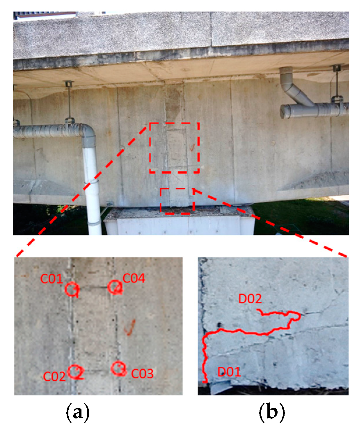
| Rectangular Box Location | Coordinates (x, y, z) (m) | Side Location | Length (m) | Damage Situation |
| C01 | (−0.141, −0.264, −4.700) | Left | 0.738 | Connected concrete crack |
| C02 | (−0.108, −0.912, −4.348) | Bottom | 0.355 | |
| C03 | (0.245, −0.880, −4.324) | Right | 0.727 | |
| C04 | (0.236, −0.240, −4.669) | Top | 0.378 | |
| Location | Coordinates (x, y, z) (m) | Crack Length (m) | Crack Width (mm) | Damage Situation |
| Starting point (D01) | (0.477, −0.996, −4.233) | 0.421 | 3.9 | Unconnected concrete cracks |
| End point (D02) | (0.615, −0.904, −4.266) |
| Side Location | Length (m) | Error (m) | Relative Error | Damage Situation |
|---|---|---|---|---|
| Left | 0.738 | 0.011 | 1.5% | Connected concrete crack |
| Right | 0.727 | |||
| Bottom | 0.355 | 0.023 | 6.1% | |
| Top | 0.378 |
| Location | Coordinates (x, y, z) (m) | Side Location | Length (m) | Damage Situation |
|---|---|---|---|---|
| E01 | (−1.408, −1.217, −4.163) | Left | 0.638 | Refilled concrete |
| E02 | (−1.140, −1.744, −4.403) | Bottom | 0.910 | |
| E03 | (−0.338, −1.528, −4.031) | Right | 0.619 | |
| E04 | (−0.584, −1.013, −3.791) | Top | 0.927 |
| Side Length Location | Length (m) | Error (m) | Relative Error | Damage Situation |
|---|---|---|---|---|
| Left | 0.638 | 0.019 | 3.0% | Refilled concrete |
| Right | 0.619 | |||
| Bottom | 0.910 | 0.017 | 1.8% | |
| Top | 0.927 |
| Location | Coordinates (x, y, z) (m) | Side Location | Length (m) | Damage Situation |
|---|---|---|---|---|
| A01 | (−0.601, 0.211, −2.487) | Left | 0.230 | Incomplete concrete grouting (hive phenomenon) |
| A02 | (−0.627, −0.016, −2.514) | Bottom | 0.383 | |
| A03 | (−0.245, −0.049, −2.523) | Right | 0.264 | |
| A04 | (−0.232, 0.213, −2.492) | Top | 0.369 | |
| B01 | (0.303, 0.271, −2.491) | Left | 0.638 | Refilled concrete |
| B02 | (0.204, −0.355, −2.566) | Bottom | 0.319 | |
| B03 | (0.518, −0.408, −2.576) | Right | 0.643 | |
| B04 | (0.618, 0.223, −2.501) | Top | 0.319 |
| Side Length Location | Length (m) | Error (m) | Relative Error | Damage Situation |
|---|---|---|---|---|
| Left | 0.638 | 0.005 | 0.8% | Refilled concrete |
| Right | 0.643 | |||
| Bottom | 0.319 | 0.000 | 0.0% | |
| Top | 0.319 |
Publisher’s Note: MDPI stays neutral with regard to jurisdictional claims in published maps and institutional affiliations. |
© 2022 by the authors. Licensee MDPI, Basel, Switzerland. This article is an open access article distributed under the terms and conditions of the Creative Commons Attribution (CC BY) license (https://creativecommons.org/licenses/by/4.0/).
Share and Cite
Kao, S.-P.; Wang, F.-L.; Lin, J.-S.; Tsai, J.; Chu, Y.-D.; Hung, P.-S. Bridge Crack Inspection Efficiency of an Unmanned Aerial Vehicle System with a Laser Ranging Module. Sensors 2022, 22, 4469. https://doi.org/10.3390/s22124469
Kao S-P, Wang F-L, Lin J-S, Tsai J, Chu Y-D, Hung P-S. Bridge Crack Inspection Efficiency of an Unmanned Aerial Vehicle System with a Laser Ranging Module. Sensors. 2022; 22(12):4469. https://doi.org/10.3390/s22124469
Chicago/Turabian StyleKao, Szu-Pyng, Feng-Liang Wang, Jhih-Sian Lin, Jichiang Tsai, Yi-De Chu, and Pen-Shan Hung. 2022. "Bridge Crack Inspection Efficiency of an Unmanned Aerial Vehicle System with a Laser Ranging Module" Sensors 22, no. 12: 4469. https://doi.org/10.3390/s22124469
APA StyleKao, S.-P., Wang, F.-L., Lin, J.-S., Tsai, J., Chu, Y.-D., & Hung, P.-S. (2022). Bridge Crack Inspection Efficiency of an Unmanned Aerial Vehicle System with a Laser Ranging Module. Sensors, 22(12), 4469. https://doi.org/10.3390/s22124469