
A Novel Machine Learning Approach for Severity Classification of Diabetic Foot Complications Using Thermogram Images

 ,
,  , , ,
, , ,  , , ,
, , ,  , and
, and 
Abstract
:1. Introduction
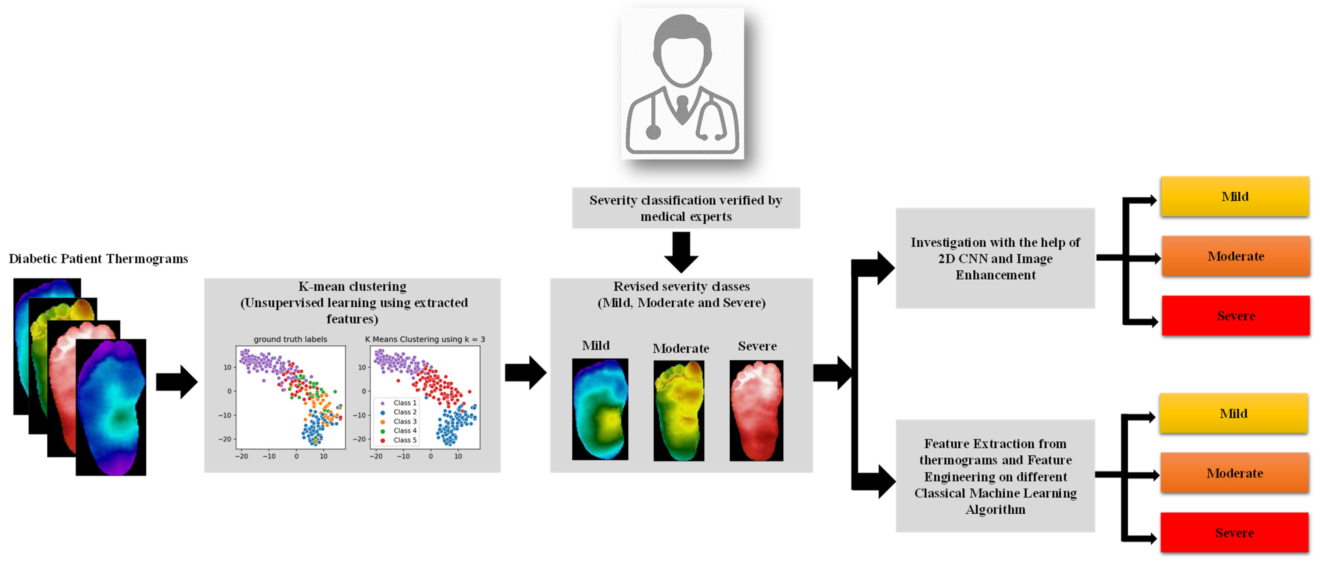
2. Methodology
2.1. Dataset
2.2. K-Mean Clustering Unsupervised Classification
- Pre-processing: Preparing the image so that it could be fed properly to the CNN model.
- Feature extraction: Using a pre-trained CNN model to extract the underlying features from a specific layer.
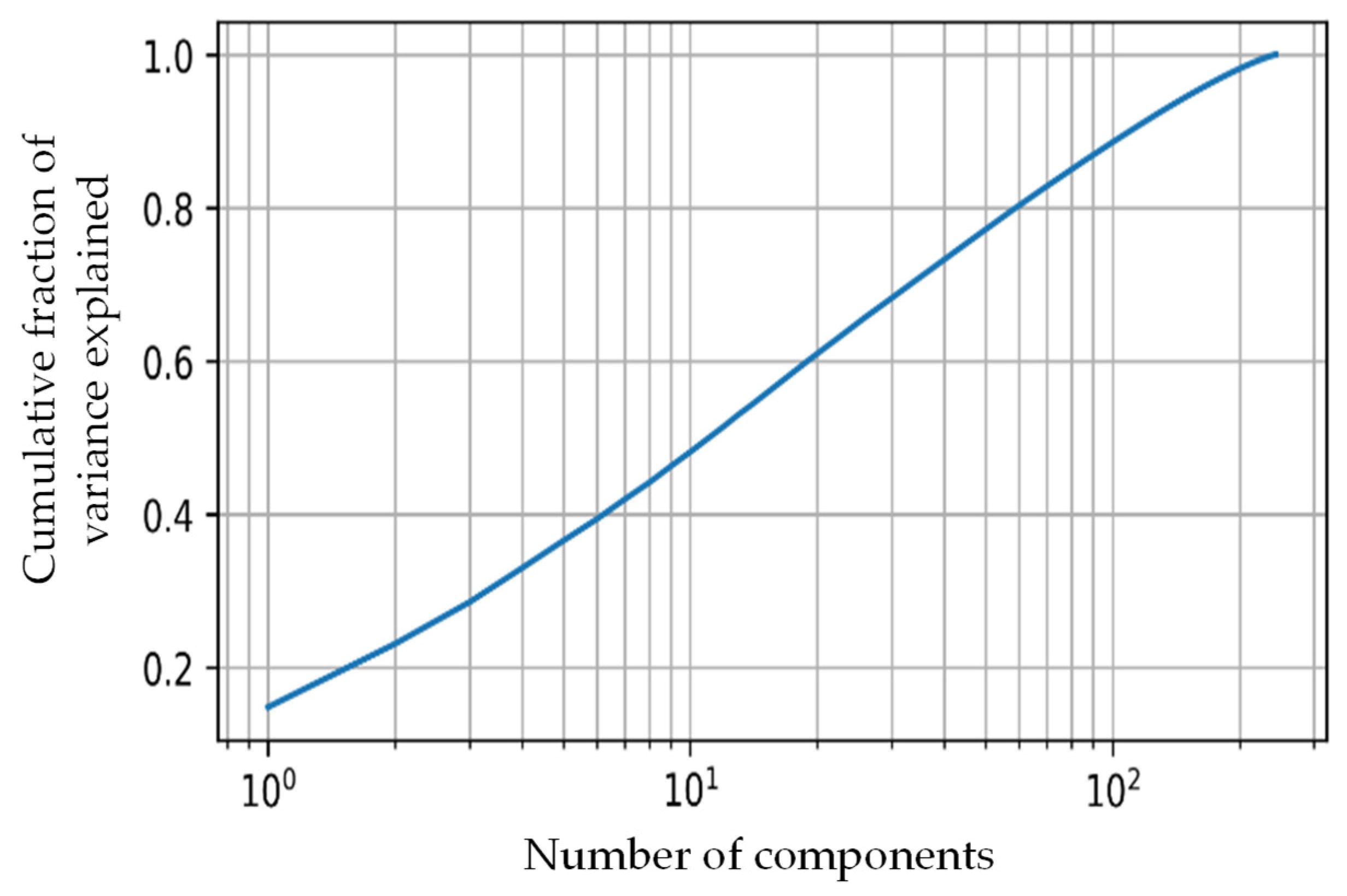
- Dimensionality reduction: Using principal component analysis (PCA) [55] to reduce the noise in the feature space and reduce the dimensionality
- Clustering: Using K-mean to cluster the images based on similar features.
| Algorithm 1: K-mean clustering | ||
| Input | : | Feature matrix, number of centroids (k) |
| Output | : | Trained model |
| 1: | for to do | |
| 2: | Assign each point with the centroid that it is closest to in latent space; | |
| 3: | Recalculate the position of the clusters () to be equal to the mean position of all of its associated points; | |
| 4: | ifthen | |
| 5: | break; | |
| 6: | ++; | |
| 7: | end for | |
2.3. Two-Dimensional CNN-Based Classification
2.4. Classical Machine Learning Approach
2.4.1. Extracted Features and Feature Reduction
2.4.2. Machine Learning Classifiers
2.4.3. Classical Machine Learning Approach 1: Optimal Combination of Feature Ranking, Number of Features
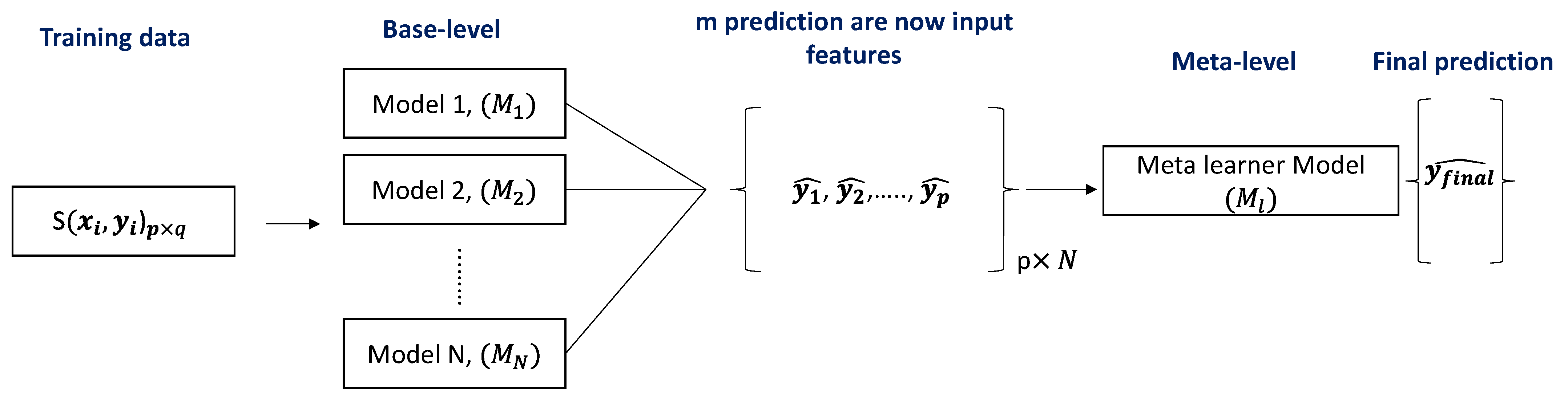
2.4.4. Classical Machine Learning Approach 2: Stacking-Based Classification
2.5. Performance Evaluation and Classification Scheme
3. Experimental Results
3.1. K-Mean Clustering Unsupervised Classification
3.2. Classical Machine Learning-Based Classification
3.2.1. Classical Machine Learning Approach 1: Optimal Combination of Feature Ranking, Number of Features
3.2.2. Classical Machine Learning Approach 2: Stacking-Based Classification
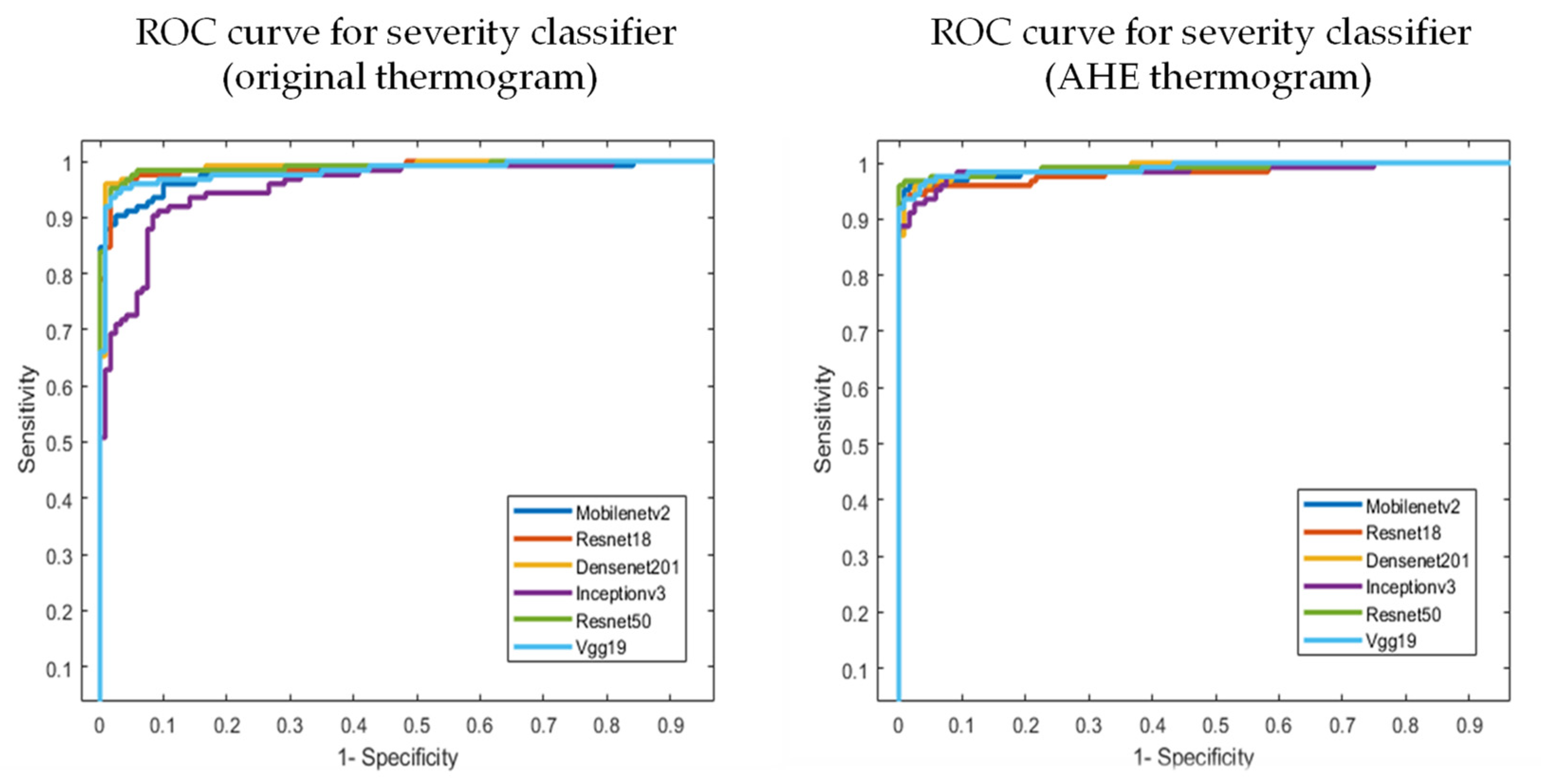
3.3. Two-Dimensional CNN-Based Classification
4. Discussion
5. Conclusions
Supplementary Materials
Author Contributions
Funding
Institutional Review Board Statement
Informed Consent Statement
Data Availability Statement
Conflicts of Interest
References
- Cho, N.; Kirigia, J.; Mbanya, J.; Ogurstova, K.; Guariguata, L.; Rathmann, W. IDF Diabetes Atlas, 8th ed.; International Diabetes Federation: Brussels, Belgium, 2015; p. 160. [Google Scholar]
- Sims, D.S., Jr.; Cavanagh, P.R.; Ulbrecht, J.S. Risk factors in the diabetic foot: Recognition and management. Phys. Ther. 1988, 68, 1887–1902. [Google Scholar] [CrossRef] [PubMed]
- Iversen, M.M.; Tell, G.S.; Riise, T.; Hanestad, B.R.; Østbye, T.; Graue, M.; Midthjell, K. History of foot ulcer increases mortality among individuals with diabetes: Ten-year follow-up of the Nord-Trøndelag Health Study, Norway. Diabetes Care 2009, 32, 2193–2199. [Google Scholar] [CrossRef] [PubMed] [Green Version]
- Singh, G.; Chawla, S. Amputation in diabetic patients. Med. J. Armed Forces India 2006, 62, 36–39. [Google Scholar] [CrossRef] [Green Version]
- Armstrong, D.G.; Boulton, A.J.; Bus, S.A. Diabetic foot ulcers and their recurrence. N. Engl. J. Med. 2017, 376, 2367–2375. [Google Scholar] [CrossRef]
- Ponirakis, G.; Elhadd, T.; Chinnaiyan, S.; Dabbous, Z.; Siddiqui, M.; Al-muhannadi, H.; Petropoulos, I.N.; Khan, A.; Ashawesh, K.A.; Dukhan, K.M.O. Prevalence and management of diabetic neuropathy in secondary care in Qatar. Diabetes/Metab. Res. Rev. 2020, 36, e3286. [Google Scholar] [CrossRef]
- Ananian, C.E.; Dhillon, Y.S.; Van Gils, C.C.; Lindsey, D.C.; Otto, R.J.; Dove, C.R.; Pierce, J.T.; Saunders, M.C. A multicenter, randomized, single-blind trial comparing the efficacy of viable cryopreserved placental membrane to human fibroblast-derived dermal substitute for the treatment of chronic diabetic foot ulcers. Wound Repair Regen. 2018, 26, 274–283. [Google Scholar] [CrossRef]
- Peter-Riesch, B. The diabetic foot: The never-ending challenge. Nov. Diabetes 2016, 31, 108–134. [Google Scholar]
- Ladyzynski, P.; Foltynski, P.; Molik, M.; Tarwacka, J.; Migalska-Musial, K.; Mlynarczuk, M.; Wojcicki, J.M.; Krzymien, J.; Karnafel, W. Area of the diabetic ulcers estimated applying a foot scanner–based home telecare system and three reference methods. Diabetes Technol. Ther. 2011, 13, 1101–1107. [Google Scholar] [CrossRef]
- Bluedrop Medical. Available online: https://bluedropmedical.com/ (accessed on 1 April 2022).
- Sugama, J.; Matsui, Y.; Sanada, H.; Konya, C.; Okuwa, M.; Kitagawa, A. A study of the efficiency and convenience of an advanced portable Wound Measurement System (VISITRAKTM). J. Clin. Nurs. 2007, 16, 1265–1269. [Google Scholar] [CrossRef]
- Molik, M.; Foltynski, P.; Ladyzynski, P.; Tarwacka, J.; Migalska-Musial, K.; Ciechanowska, A.; Sabalinska, S.; Mlynarczuk, M.; Wojcicki, J.M.; Krzymien, J. Comparison of the wound area assessment methods in the diabetic foot syndrome. Biocybernet. Biomed. Eng. 2010, 30, 3–15. [Google Scholar]
- Reyzelman, A.M.; Koelewyn, K.; Murphy, M.; Shen, X.; Yu, E.; Pillai, R.; Fu, J.; Scholten, H.J.; Ma, R. Continuous temperature-monitoring socks for home use in patients with diabetes: Observational study. J. Med. Internet Res. 2018, 20, e12460. [Google Scholar] [CrossRef] [PubMed] [Green Version]
- Frykberg, R.G.; Gordon, I.L.; Reyzelman, A.M.; Cazzell, S.M.; Fitzgerald, R.H.; Rothenberg, G.M.; Bloom, J.D.; Petersen, B.J.; Linders, D.R.; Nouvong, A. Feasibility and efficacy of a smart mat technology to predict development of diabetic plantar ulcers. Diabetes Care 2017, 40, 973–980. [Google Scholar] [CrossRef] [PubMed] [Green Version]
- Nagase Inagaki, F.N. The Impact of Diabetic Foot Problems on Health-Related Quality of Life of People with Diabetes. Master’s Thesis, University of Alberta, Edmonton, AB, Canada, 2017. [Google Scholar]
- van Doremalen, R.F.; van Netten, J.J.; van Baal, J.G.; Vollenbroek-Hutten, M.M.; van der Heijden, F. Infrared 3D thermography for inflammation detection in diabetic foot disease: A proof of concept. J. Diabetes Sci. Technol. 2020, 14, 46–54. [Google Scholar] [CrossRef]
- Crisologo, P.A.; Lavery, L.A. Remote home monitoring to identify and prevent diabetic foot ulceration. Ann. Transl. Med. 2017, 5, 430. [Google Scholar] [CrossRef]
- Yang, J.; Yin, P.; Zhou, M.; Ou, C.-Q.; Li, M.; Liu, Y.; Gao, J.; Chen, B.; Liu, J.; Bai, L. The effect of ambient temperature on diabetes mortality in China: A multi-city time series study. Sci. Total Environ. 2016, 543, 75–82. [Google Scholar] [CrossRef]
- Song, X.; Jiang, L.; Zhang, D.; Wang, X.; Ma, Y.; Hu, Y.; Tang, J.; Li, X.; Huang, W.; Meng, Y. Impact of short-term exposure to extreme temperatures on diabetes mellitus morbidity and mortality? A systematic review and meta-analysis. Environ. Sci. Pollut. Res. 2021, 28, 58035–58049. [Google Scholar] [CrossRef]
- Foltyński, P.; Mrozikiewicz-Rakowska, B.; Ładyżyński, P.; Wójcicki, J.M.; Karnafel, W. The influence of ambient temperature on foot temperature in patients with diabetic foot ulceration. Biocybern. Biomed. Eng. 2014, 34, 178–183. [Google Scholar] [CrossRef]
- Albers, J.W.; Jacobson, R. Decompression nerve surgery for diabetic neuropathy: A structured review of published clinical trials. Diabetes Metab. Syndr. Obes. Targets Ther. 2018, 11, 493. [Google Scholar] [CrossRef] [Green Version]
- Hernandez-Contreras, D.; Peregrina-Barreto, H.; Rangel-Magdaleno, J.; Gonzalez-Bernal, J. Narrative review: Diabetic foot and infrared thermography. Infrared Phys. Technol. 2016, 78, 105–117. [Google Scholar] [CrossRef]
- Ring, F. Thermal imaging today and its relevance to diabetes. J. Diabetes Sci. Technol. 2010, 4, 857–862. [Google Scholar] [CrossRef] [PubMed] [Green Version]
- Chan, A.W.; MacFarlane, I.A.; Bowsher, D.R. Contact thermography of painful diabetic neuropathic foot. Diabetes Care 1991, 14, 918–922. [Google Scholar] [CrossRef] [PubMed]
- Nagase, T.; Sanada, H.; Takehara, K.; Oe, M.; Iizaka, S.; Ohashi, Y.; Oba, M.; Kadowaki, T.; Nakagami, G. Variations of plantar thermographic patterns in normal controls and non-ulcer diabetic patients: Novel classification using angiosome concept. J. Plast. Reconstr. Aesthetic Surg. 2011, 64, 860–866. [Google Scholar] [CrossRef] [PubMed]
- Mori, T.; Nagase, T.; Takehara, K.; Oe, M.; Ohashi, Y.; Amemiya, A.; Noguchi, H.; Ueki, K.; Kadowaki, T.; Sanada, H. Morphological Pattern Classification System for Plantar Thermography of Patients with Diabetes; SAGE Publications Sage CA: Los Angeles, CA, USA, 2013. [Google Scholar]
- Jones, B.F. A reappraisal of the use of infrared thermal image analysis in medicine. IEEE Trans. Med. Imaging 1998, 17, 1019–1027. [Google Scholar] [CrossRef] [PubMed]
- Kaabouch, N.; Chen, Y.; Anderson, J.; Ames, F.; Paulson, R. Asymmetry analysis based on genetic algorithms for the prediction of foot ulcers. In Visualization and Data Analysis 2009; International Society for Optics and Photonics: Bellingham, WA, USA, 2009; p. 724304. [Google Scholar]
- Kaabouch, N.; Chen, Y.; Hu, W.-C.; Anderson, J.W.; Ames, F.; Paulson, R. Enhancement of the asymmetry-based overlapping analysis through features extraction. J. Electron. Imaging 2011, 20, 013012. [Google Scholar] [CrossRef]
- Liu, C.; van Netten, J.J.; Van Baal, J.G.; Bus, S.A.; van Der Heijden, F. Automatic detection of diabetic foot complications with infrared thermography by asymmetric analysis. J. Biomed. Opt. 2015, 20, 026003. [Google Scholar] [CrossRef] [Green Version]
- Hernandez-Contreras, D.; Peregrina-Barreto, H.; Rangel-Magdaleno, J.; Ramirez-Cortes, J.; Renero-Carrillo, F. Automatic classification of thermal patterns in diabetic foot based on morphological pattern spectrum. Infrared Phys. Technol. 2015, 73, 149–157. [Google Scholar] [CrossRef]
- Hernandez-Contreras, D.; Peregrina-Barreto, H.; Rangel-Magdaleno, J.; Gonzalez-Bernal, J.; Altamirano-Robles, L. A quantitative index for classification of plantar thermal changes in the diabetic foot. Infrared Phys. Technol. 2017, 81, 242–249. [Google Scholar] [CrossRef]
- Hernandez-Contreras, D.A.; Peregrina-Barreto, H.; Rangel-Magdaleno, J.D.J.; Orihuela-Espina, F. Statistical approximation of plantar temperature distribution on diabetic subjects based on beta mixture model. IEEE Access 2019, 7, 28383–28391. [Google Scholar] [CrossRef]
- Kamavisdar, P.; Saluja, S.; Agrawal, S. A survey on image classification approaches and techniques. Int. J. Adv. Res. Comput. Commun. Eng. 2013, 2, 1005–1009. [Google Scholar]
- Ren, J. ANN vs. SVM: Which one performs better in classification of MCCs in mammogram imaging. Knowl.-Based Syst. 2012, 26, 144–153. [Google Scholar] [CrossRef] [Green Version]
- Lu, D.; Weng, Q. A survey of image classification methods and techniques for improving classification performance. Int. J. Remote Sens. 2007, 28, 823–870. [Google Scholar] [CrossRef]
- Khandakar, A.; Chowdhury, M.E.; Reaz, M.B.I.; Ali, S.H.M.; Hasan, M.A.; Kiranyaz, S.; Rahman, T.; Alfkey, R.; Bakar, A.A.A.; Malik, R.A. A machine learning model for early detection of diabetic foot using thermogram images. Comput. Biol. Med. 2021, 137, 104838. [Google Scholar] [CrossRef] [PubMed]
- Cruz-Vega, I.; Hernandez-Contreras, D.; Peregrina-Barreto, H.; Rangel-Magdaleno, J.d.J.; Ramirez-Cortes, J.M. Deep Learning Classification for Diabetic Foot Thermograms. Sensors 2020, 20, 1762. [Google Scholar] [CrossRef] [Green Version]
- Hernandez-Contreras, D.A.; Peregrina-Barreto, H.; de Jesus Rangel-Magdaleno, J.; Renero-Carrillo, F.J. Plantar thermogram database for the study of diabetic foot complications. IEEE Access 2019, 7, 161296–161307. [Google Scholar] [CrossRef]
- Maldonado, H.; Bayareh, R.; Torres, I.; Vera, A.; Gutiérrez, J.; Leija, L. Automatic detection of risk zones in diabetic foot soles by processing thermographic images taken in an uncontrolled environment. Infrared Phys. Technol. 2020, 105, 103187. [Google Scholar] [CrossRef]
- Saminathan, J.; Sasikala, M.; Narayanamurthy, V.; Rajesh, K.; Arvind, R. Computer aided detection of diabetic foot ulcer using asymmetry analysis of texture and temperature features. Infrared Phys. Technol. 2020, 105, 103219. [Google Scholar] [CrossRef]
- Adam, M.; Ng, E.Y.; Oh, S.L.; Heng, M.L.; Hagiwara, Y.; Tan, J.H.; Tong, J.W.; Acharya, U.R. Automated detection of diabetic foot with and without neuropathy using double density-dual tree-complex wavelet transform on foot thermograms. Infrared Phys. Technol. 2018, 92, 270–279. [Google Scholar] [CrossRef]
- Adam, M.; Ng, E.Y.; Oh, S.L.; Heng, M.L.; Hagiwara, Y.; Tan, J.H.; Tong, J.W.; Acharya, U.R. Automated characterization of diabetic foot using nonlinear features extracted from thermograms. Infrared Phys. Technol. 2018, 89, 325–337. [Google Scholar] [CrossRef]
- Gururajarao, S.B.; Venkatappa, U.; Shivaram, J.M.; Sikkandar, M.Y.; Al Amoudi, A. Infrared thermography and soft computing for diabetic foot assessment. In Machine Learning in Bio-Signal Analysis and Diagnostic Imaging; Elsevier: Amsterdam, The Netherlands, 2019; pp. 73–97. [Google Scholar]
- Etehadtavakol, M.; Emrani, Z.; Ng, E.Y.K. Rapid extraction of the hottest or coldest regions of medical thermographic images. Med. Biol. Eng. Comput. 2019, 57, 379–388. [Google Scholar] [CrossRef]
- Wang, Y.; Huang, R.; Huang, G.; Song, S.; Wu, C. Collaborative learning with corrupted labels. Neural Netw. 2020, 125, 205–213. [Google Scholar] [CrossRef] [PubMed]
- Aradillas, J.C.; Murillo-Fuentes, J.J.; Olmos, P.M. Improving offline HTR in small datasets by purging unreliable labels. In Proceedings of the 2020 17th International Conference on Frontiers in Handwriting Recognition (ICFHR), Dortmund, Germany, 8–10 September 2020; pp. 25–30. [Google Scholar]
- Hu, W.; Huang, Y.; Zhang, F.; Li, R. Noise-tolerant paradigm for training face recognition CNNs. In Proceedings of the IEEE/CVF Conference on Computer Vision and Pattern Recognition, Long Beach, CA, USA, 15–20 June 2019; pp. 11887–11896. [Google Scholar]
- Ding, Y.; Wang, L.; Fan, D.; Gong, B. A semi-supervised two-stage approach to learning from noisy labels. In Proceedings of the 2018 IEEE Winter Conference on Applications of Computer Vision (WACV), Lake Tahoe, NV, USA, 12–15 March 2018; pp. 1215–1224. [Google Scholar]
- Fraiwan, L.; AlKhodari, M.; Ninan, J.; Mustafa, B.; Saleh, A.; Ghazal, M. Diabetic foot ulcer mobile detection system using smart phone thermal camera: A feasibility study. Biomed. Eng. Online 2017, 16, 117. [Google Scholar] [CrossRef] [Green Version]
- Alzubaidi, L.; Fadhel, M.A.; Oleiwi, S.R.; Al-Shamma, O.; Zhang, J. DFU_QUTNet: Diabetic foot ulcer classification using novel deep convolutional neural network. Multimed. Tools Appl. 2020, 79, 15655–15677. [Google Scholar] [CrossRef]
- Tulloch, J.; Zamani, R.; Akrami, M. Machine learning in the prevention, diagnosis and management of diabetic foot ulcers: A systematic review. IEEE Access 2020, 8, 198977–199000. [Google Scholar] [CrossRef]
- Yadav, J.; Sharma, M. A Review of K-mean Algorithm. Int. J. Eng. Trends Technol. 2013, 4, 2972–2976. [Google Scholar]
- Taylor, G.I.; Palmer, J.H. Angiosome theory. Br. J. Plast. Surg. 1992, 45, 327–328. [Google Scholar] [CrossRef]
- Xie, X. Principal Component Analysis. 2019. Available online: https://www.google.com/url?sa=t&rct=j&q=&esrc=s&source=web&cd=&ved=2ahUKEwi25YTAgtn3AhUGmlYBHdtqDwYQFnoECAMQAQ&url=https%3A%2F%2Fwww.ics.uci.edu%2F~xhx%2Fcourses%2FCS273P%2F12-pca-273p.pdf&usg=AOvVaw1xc-uIUhsccvWmCWGL411_ (accessed on 1 August 2021).
- Keras. Available online: https://keras.io/ (accessed on 1 August 2021).
- Russakovsky, O.; Deng, J.; Su, H.; Krause, J.; Satheesh, S.; Ma, S.; Huang, Z.; Karpathy, A.; Khosla, A.; Bernstein, M. Imagenet large scale visual recognition challenge. Int. J. Comput. Vis. 2015, 115, 211–252. [Google Scholar] [CrossRef] [Green Version]
- Simonyan, K.; Zisserman, A. Very deep convolutional networks for large-scale image recognition. arXiv 2014, arXiv:1409.1556. [Google Scholar]
- Cohn, R.; Holm, E. Unsupervised machine learning via transfer learning and k-means clustering to classify materials image data. Integr. Mater. Manuf. Innov. 2021, 10, 231–244. [Google Scholar] [CrossRef]
- Song, K.; Yan, Y. A noise robust method based on completed local binary patterns for hot-rolled steel strip surface defects. Appl. Surf. Sci. 2013, 285, 858–864. [Google Scholar] [CrossRef]
- Blankenship, S.M.; Campbell, M.R.; Hess, J.E.; Hess, M.A.; Kassler, T.W.; Kozfkay, C.C.; Matala, A.P.; Narum, S.R.; Paquin, M.M.; Small, M.P. Major lineages and metapopulations in Columbia River Oncorhynchus mykiss are structured by dynamic landscape features and environments. Trans. Am. Fish. Soc. 2011, 140, 665–684. [Google Scholar] [CrossRef]
- Hamed, M.A.R. Application of Surface Water Quality Classification Models Using PRINCIPAL Components Analysis and Cluster Analysis. 2019. Available online: https://ssrn.com/abstract=3364401 (accessed on 1 August 2021).
- Malik, H.; Hemmati, H.; Hassan, A.E. Automatic detection of performance deviations in the load testing of large scale systems. In Proceedings of the 2013 35th International Conference on Software Engineering (ICSE), San Francisco, CA, USA, 18–26 May 2013; pp. 1012–1021. [Google Scholar]
- Toe, M.T.; Kanzaki, M.; Lien, T.-H.; Cheng, K.-S. Spatial and temporal rainfall patterns in Central Dry Zone, Myanmar-A hydrological cross-scale analysis. Terr. Atmos. Ocean. Sci. 2017, 28, 425–436. [Google Scholar] [CrossRef] [Green Version]
- Lloyd, S. Least squares quantization in PCM. IEEE Trans. Inf. Theory 1982, 28, 129–137. [Google Scholar] [CrossRef] [Green Version]
- Bock, H.-H. Clustering methods: A history of k-means algorithms. In Selected Contributions in Data Analysis and Classification; Springer: Berlin/Heidelberg, Germany, 2007; pp. 161–172. [Google Scholar]
- Jain, A.K. Data clustering: 50 years beyond K-means. Pattern Recognit. Lett. 2010, 31, 651–666. [Google Scholar] [CrossRef]
- Arthur, D.; Vassilvitskii, S. k-Means++: The Advantages of Careful Seeding; ACM Digital Library: Stanford, CA, USA, 2006. [Google Scholar]
- Anwar, S.M.; Majid, M.; Qayyum, A.; Awais, M.; Alnowami, M.; Khan, M.K. Medical image analysis using convolutional neural networks: A review. J. Med. Syst. 2018, 42, 226. [Google Scholar] [CrossRef] [Green Version]
- Tahir, A.M.; Qiblawey, Y.; Khandakar, A.; Rahman, T.; Khurshid, U.; Musharavati, F.; Islam, M.; Kiranyaz, S.; Al-Maadeed, S.; Chowdhury, M.E. Deep learning for reliable classification of COVID-19, MERS, and SARS from chest X-ray images. Cogn. Comput. 2022, 1–21. [Google Scholar] [CrossRef]
- Deng, J.; Dong, W.; Socher, R.; Li, L.-J.; Li, K.; Fei-Fei, L. Imagenet: A large-scale hierarchical image database. In Proceedings of the 2009 IEEE Conference on Computer Vision and Pattern Recognition, Miami, FL, USA, 20–25 June 2009; pp. 248–255. [Google Scholar]
- Mishra, M.; Menon, H.; Mukherjee, A. Characterization of S1 and S2 Heart Sounds Using Stacked Autoencoder and Convolutional Neural Network. IEEE Trans. Instrum. Meas. 2018, 68, 3211–3220. [Google Scholar] [CrossRef]
- Szegedy, C.; Vanhoucke, V.; Ioffe, S.; Shlens, J.; Wojna, Z. Rethinking the inception architecture for computer vision. In Proceedings of the IEEE Conference on Computer Vision and Pattern Recognition, Las Vegas, NV, USA, 27–30 June 2016; pp. 2818–2826. [Google Scholar]
- Sandler, M.; Howard, A.; Zhu, M.; Zhmoginov, A.; Chen, L.-C. Mobilenetv2: Inverted residuals and linear bottlenecks. In Proceedings of the IEEE Conference on Computer Vision and Pattern Recognition, Salt Lake City, UT, USA, 18–22 June 2018; pp. 4510–4520. [Google Scholar]
- Zimmerman, J.B.; Pizer, S.M.; Staab, E.V.; Perry, J.R.; McCartney, W.; Brenton, B.C. An evaluation of the effectiveness of adaptive histogram equalization for contrast enhancement. IEEE Trans. Med. Imaging 1988, 7, 304–312. [Google Scholar] [CrossRef] [Green Version]
- Tawsifur Rahman, A.K.; Qiblawey, Y.; Tahir, A.; Kiranyaz, S.; Saad, M.T.I.; Kashem, B.A.; Al Maadeed, S.; Zughaier, S.M.; Khan, M.E.H.C.M.S. Exploring the Effect of Image Enhancement Techniques on COVID-19 Detection using Chest X-rays Images. arXiv 2020, arXiv:2012.02238. [Google Scholar]
- Chowdhury, M.H.; Shuzan, M.N.I.; Chowdhury, M.E.; Mahbub, Z.B.; Uddin, M.M.; Khandakar, A.; Reaz, M.B.I. Estimating blood pressure from the photoplethysmogram signal and demographic features using machine learning techniques. Sensors 2020, 20, 3127. [Google Scholar] [CrossRef]
- Hall, M.A. Correlation-Based Feature Selection for Machine Learning. Ph.D. Thesis, The University of Waikato, Hamilton, New Zealand, 1999. [Google Scholar]
- Multilayer Perceptron. Available online: https://en.wikipedia.org/wiki/Multilayer_perceptron (accessed on 2 March 2022).
- Zhang, Y. Support vector machine classification algorithm and its application. In Proceedings of the International Conference on Information Computing and Applications; Springer: Berlin/Heidelberg, Germany, 2012; pp. 179–186. [Google Scholar]
- Pal, M. Random forest classifier for remote sensing classification. Int. J. Remote Sens. 2005, 26, 217–222. [Google Scholar] [CrossRef]
- Sharaff, A.; Gupta, H. Extra-tree classifier with metaheuristics approach for email classification. In Advances in Computer Communication and Computational Sciences; Springer: Berlin/Heidelberg, Germany, 2019; pp. 189–197. [Google Scholar]
- Bahad, P.; Saxena, P. Study of adaboost and gradient boosting algorithms for predictive analytics. In Proceedings of the International Conference on Intelligent Computing and Smart Communication 2019; Springer: Singapore, 2020; pp. 235–244. [Google Scholar]
- Logistic Regression. Available online: https://en.wikipedia.org/wiki/Logistic_regression (accessed on 2 March 2022).
- Liao, Y.; Vemuri, V.R. Use of k-nearest neighbor classifier for intrusion detection. Comput. Secur. 2002, 21, 439–448. [Google Scholar] [CrossRef]
- Shi, X.; Li, Q.; Qi, Y.; Huang, T.; Li, J. An accident prediction approach based on XGBoost. In Proceedings of the 2017 12th International Conference on Intelligent Systems and Knowledge Engineering (ISKE), Nanjing, China, 24–26 November 2017; pp. 1–7. [Google Scholar]
- Bobkov, V.; Bobkova, A.; Porshnev, S.; Zuzin, V. The application of ensemble learning for delineation of the left ventricle on echocardiographic records. In Proceedings of the 2016 Dynamics of Systems, Mechanisms and Machines (Dynamics), Omsk, Russia, 15–17 November 2016; pp. 1–5. [Google Scholar]
- Gu, Q.; Li, Z.; Han, J. Linear discriminant dimensionality reduction. In Proceedings of the Joint European Conference on Machine Learning and Knowledge Discovery in Databases; Springer: Berlin/Heidelberg, Germany, 2011; pp. 549–564. [Google Scholar]
- Chen, T.; He, T.; Benesty, M.; Khotilovich, V.; Tang, Y. Xgboost: Extreme Gradient Boosting; R Package Version 0.4-2; 2015; pp. 1–4. Available online: https://www.google.com/url?sa=t&rct=j&q=&esrc=s&source=web&cd=&cad=rja&uact=8&ved=2ahUKEwjGh7GmhNn3AhU6tlYBHRGJBQYQFnoECAMQAQ&url=https%3A%2F%2Fcran.microsoft.com%2Fsnapshot%2F2015-10-20%2Fweb%2Fpackages%2Fxgboost%2Fxgboost.pdf&usg=AOvVaw1w25OwKdxLEfpj0rZsvL6J (accessed on 1 March 2022).
- Saeys, Y.; Abeel, T.; Van de Peer, Y. Robust feature selection using ensemble feature selection techniques. In Proceedings of the Joint European Conference on Machine Learning and Knowledge Discovery in Databases; Springer: Berlin/Heidelberg, Germany, 2008; pp. 313–325. [Google Scholar]
- Petković, M.; Kocev, D.; Džeroski, S. Feature ranking for multi-target regression. Mach. Learn. 2020, 109, 1179–1204. [Google Scholar] [CrossRef]
- Yusof, A.R.; Udzir, N.I.; Selamat, A.; Hamdan, H.; Abdullah, M.T. Adaptive feature selection for denial of services (DoS) attack. In Proceedings of the 2017 IEEE Conference on Application, Information and Network Security (AINS), Miri, Malaysia, 13–14 November 2017; pp. 81–84. [Google Scholar]
- Saidi, R.; Bouaguel, W.; Essoussi, N. Hybrid feature selection method based on the genetic algorithm and pearson correlation coefficient. In Machine Learning Paradigms: Theory and Application; Springer: Berlin/Heidelberg, Germany, 2019; pp. 3–24. [Google Scholar]
- Lin, X.; Yang, F.; Zhou, L.; Yin, P.; Kong, H.; Xing, W.; Lu, X.; Jia, L.; Wang, Q.; Xu, G. A support vector machine-recursive feature elimination feature selection method based on artificial contrast variables and mutual information. J. Chromatogr. B 2012, 910, 149–155. [Google Scholar] [CrossRef]
- Bursac, Z.; Gauss, C.H.; Williams, D.K.; Hosmer, D.W. Purposeful selection of variables in logistic regression. Source Code Biol. Med. 2008, 3, 17. [Google Scholar] [CrossRef] [Green Version]
- Leevy, J.L.; Hancock, J.; Zuech, R.; Khoshgoftaar, T.M. Detecting cybersecurity attacks using different network features with lightgbm and xgboost learners. In Proceedings of the 2020 IEEE Second International Conference on Cognitive Machine Intelligence (CogMI), Atlanta, GA, USA, 28–31 October 2020; pp. 190–197. [Google Scholar]
- Taha, A.A.; Hanbury, A. Metrics for evaluating 3D medical image segmentation: Analysis, selection, and tool. BMC Med. Imaging 2015, 15, 29. [Google Scholar] [CrossRef] [Green Version]
- Rahman, T.; Khandakar, A.; Kadir, M.A.; Islam, K.R.; Islam, K.F.; Mazhar, R.; Hamid, T.; Islam, M.T.; Kashem, S.; Mahbub, Z.B. Reliable tuberculosis detection using chest X-ray with deep learning, segmentation and visualization. IEEE Access 2020, 8, 191586–191601. [Google Scholar] [CrossRef]


| Classifier | Dataset | Count of Diabetic Thermograms/Cluster Identified in the Paper | Training Dataset Details | |||
|---|---|---|---|---|---|---|
| Training (60% of the Data) Thermogram /Fold | Augmented Train Thermogram /Fold | Validation (20% of the Data) Thermogram /Fold | Test (20 % of the Data) Image/Fold | |||
| Severity | Contreras et al. [39] | Mild | 43 | 2040 | 3 | 11 |
| Moderate | 48 | 2244 | 4 | 11 | ||
| Severe | 93 | 1806 | 7 | 24 | ||
| Classifier | Feature Selection | # of Feature | Class | Accuracy | Precision | Sensitivity | F1-Score | Specificity | Inference Time (ms) |
|---|---|---|---|---|---|---|---|---|---|
| XGBoost | Random Forest | 25 | Mild | 92.59 ± 6.80 | 91.53 ± 7.23 | 94.74 ± 5.80 | 93.1 ± 6.58 | 91.94 ± 7.07 | 0.397 |
| Moderate | 92.59 ± 6.47 | 86.15 ± 8.53 | 88.89 ± 7.76 | 87.5 ± 8.17 | 93.89 ± 5.91 | ||||
| Severe | 92.59 ± 4.61 | 96.64 ± 3.17 | 93.50 ± 4.34 | 95.04 ± 3.82 | 91.67 ± 4.86 | ||||
| Overall | 92.59 ± 3.29 | 92.72 ± 3.26 | 92.59 ± 3.29 | 92.63 ± 3.28 | 92.31 ± 3.34 |
| Feature | Pearson | Chi-Square | RFE | Logistics | Random Forest | LightGBM | Total |
|---|---|---|---|---|---|---|---|
| TCI | √ | √ | √ | √ | √ | √ | 6 |
| NRT (Class 4) | √ | √ | √ | √ | √ | √ | 6 |
| NRT (Class 3) | √ | √ | √ | √ | √ | √ | 6 |
| Mean of MPA | √ | √ | √ | √ | √ | √ | 6 |
| Mean of LPA | √ | √ | √ | √ | √ | √ | 6 |
| ET of LPA | √ | √ | √ | √ | √ | √ | 6 |
| Mean of LCA | √ | √ | √ | √ | √ | √ | 6 |
| Highest Temperature | √ | √ | √ | √ | √ | √ | 6 |
| NRT (Class 2) | √ | √ | √ | √ | √ | 5 | |
| NRT (Class 1) | √ | √ | √ | √ | √ | 5 | |
| ET of LCA | √ | √ | √ | √ | √ | 5 | |
| NRT (Class 5) | √ | √ | √ | √ | 4 | ||
| STD of MPA | √ | √ | √ | √ | 4 | ||
| ETD of MPA | √ | √ | √ | √ | 4 | ||
| STD of MCA | √ | √ | √ | √ | 4 | ||
| ETD of MCA | √ | √ | √ | √ | 4 | ||
| STD of LPA | √ | √ | √ | √ | 4 | ||
| HSE of LCA | √ | √ | √ | √ | 4 | ||
| ETD of Full foot | √ | √ | √ | √ | 4 |
| Classifier | Class | Accuracy | Precision | Sensitivity | F1-Score | Specificity | Inference Time (ms) |
|---|---|---|---|---|---|---|---|
| Gradient Boost | Mild | 92.01 ± 4.98 | 91.38 ± 5.15 | 92.98 ± 4.69 | 92.17 ± 4.93 | 91.71 ± 5.06 | 0.379 |
| Moderate | 92.01 ± 4.73 | 84.50 ± 6.32 | 86.51 ± 5.97 | 85.49 ± 6.15 | 93.92 ± 4.17 | ||
| Severe | 92.01 ± 3.37 | 96.30 ± 2.35 | 94.35 ± 2.87 | 95.32 ± 2.63 | 89.58 ± 3.80 | ||
| Overall | 92.01 ± 3.40 | 92.10 ± 3.38 | 92.01 ± 3.40 | 92.04 ± 3.40 | 91.20 ± 3.55 | ||
| XGBoost | Mild | 93.24 ± 4.61 | 90.08 ± 5.49 | 95.61 ± 3.76 | 92.77 ± 4.76 | 92.51 ± 4.83 | 0.336 |
| Moderate | 93.24 ± 4.38 | 89.26 ± 5.41 | 85.71 ± 6.11 | 87.45 ± 5.78 | 95.86 ± 3.48 | ||
| Severe | 93.24 ± 3.13 | 96.75 ± 2.21 | 95.97 ± 2.45 | 96.36 ± 2.33 | 90.42 ± 3.66 | ||
| Overall | 93.24 ± 3.15 | 93.26 ± 3.15 | 93.24 ± 3.15 | 93.22 ± 3.15 | 92.31 ± 3.34 | ||
| Random Forest | Mild | 91.80 ± 5.04 | 89.19 ± 5.7 | 86.84 ± 6.21 | 88.00 ± 5.97 | 93.32 ± 4.58 | 0.327 |
| Moderate | 91.80 ± 4.79 | 90.43 ± 5.14 | 82.54 ± 6.63 | 86.31 ± 6.00 | 95.03 ± 3.80 | ||
| Severe | 91.80 ± 3.41 | 93.51 ± 3.07 | 98.79 ± 1.36 | 96.08 ± 2.42 | 84.58 ± 4.49 | ||
| Overall | 91.80 ± 3.44 | 91.71 ± 3.46 | 91.80 ± 3.44 | 91.67 ± 3.47 | 89.32 ± 3.88 | ||
| Stacking (Gradient Boost + XGBoost + Random Forest) | Mild | 94.47 ± 4.20 | 91.53 ± 5.11 | 94.74 ± 4.10 | 93.10 ± 4.65 | 94.39 ± 4.23 | 0.379 + 0.336 + 0.327 = 1.042 |
| Moderate | 94.47 ± 3.99 | 92.44 ± 4.62 | 87.30 ± 5.81 | 89.80 ± 5.29 | 96.96 ± 3.00 | ||
| Severe | 94.47 ± 2.85 | 96.81 ± 2.19 | 97.98 ± 1.75 | 97.39 ± 1.98 | 90.83 ± 3.59 | ||
| Overall | 94.47 ± 2.87 | 94.45 ± 2.87 | 94.47 ± 2.87 | 94.43 ± 2.88 | 93.25 ± 3.15 |
| Enhancement | Network | Class | Accuracy | Precision | Sensitivity | F1-Score | Specificity | Inference Time (ms) |
|---|---|---|---|---|---|---|---|---|
| Original | VGG 19 | Mild | 98.77 ± 2.86 | 98.21 ± 3.44 | 96.49 ± 4.78 | 97.34 ± 4.18 | 99.47 ± 1.88 | 7.271 |
| Moderate | 94.67 ± 5.55 | 86.76 ± 8.37 | 93.65 ± 6.02 | 90.07 ± 7.39 | 95.03 ± 5.37 | |||
| Severe | 95.90 ± 3.49 | 97.50 ± 2.75 | 94.35 ± 4.06 | 95.90 ± 3.49 | 97.5 ± 2.75 | |||
| Overall | 94.76 ± 2.82 | 94.89 ± 2.76 | 94.67 ± 2.82 | 94.73 ± 2.80 | 97.32 ± 2.03 | |||
| AHE | VGG 19 | Mild | 98.77 ± 2.86 | 96.55 ± 4.74 | 98.25 ± 3.4 | 97.39 ± 4.14 | 98.93 ± 2.67 | 8.161 |
| Moderate | 95.08 ± 5.34 | 90.48 ± 7.25 | 90.48 ± 7.25 | 90.48 ± 7.25 | 96.69 ± 4.42 | |||
| Severe | 96.31 ± 3.32 | 96.75 ± 3.12 | 95.97 ± 3.46 | 96.36 ± 3.3 | 96.67 ± 3.16 | |||
| Overall | 95.08 ± 2.71 | 95.08 ± 2.71 | 95.09 ± 2.71 | 95.08 ± 2.71 | 97.2 ± 2.07 | |||
| Gamma Correction | VGG 19 | Mild | 88.11 ± 8.40 | 90.91 ± 7.46 | 87.72 ± 8.52 | 89.29 ± 8.03 | 88.24 ± 8.36 | 9.651 |
| Moderate | 88.11 ± 7.99 | 75.71 ± 10.59 | 84.13 ± 9.02 | 79.70 ± 9.93 | 89.50 ± 7.57 | |||
| Severe | 88.11 ± 5.70 | 94.12 ± 4.14 | 90.32 ± 5.20 | 92.18 ± 4.73 | 85.83 ± 6.14 | |||
| Overall | 88.11 ± 4.06 | 88.62 ± 3.99 | 88.11 ± 4.06 | 88.28 ± 4.04 | 87.34 ± 4.17 |
Publisher’s Note: MDPI stays neutral with regard to jurisdictional claims in published maps and institutional affiliations. |
© 2022 by the authors. Licensee MDPI, Basel, Switzerland. This article is an open access article distributed under the terms and conditions of the Creative Commons Attribution (CC BY) license (https://creativecommons.org/licenses/by/4.0/).
Share and Cite
Khandakar, A.; Chowdhury, M.E.H.; Reaz, M.B.I.; Ali, S.H.M.; Kiranyaz, S.; Rahman, T.; Chowdhury, M.H.; Ayari, M.A.; Alfkey, R.; Bakar, A.A.A.; et al. A Novel Machine Learning Approach for Severity Classification of Diabetic Foot Complications Using Thermogram Images. Sensors 2022, 22, 4249. https://doi.org/10.3390/s22114249
Khandakar A, Chowdhury MEH, Reaz MBI, Ali SHM, Kiranyaz S, Rahman T, Chowdhury MH, Ayari MA, Alfkey R, Bakar AAA, et al. A Novel Machine Learning Approach for Severity Classification of Diabetic Foot Complications Using Thermogram Images. Sensors. 2022; 22(11):4249. https://doi.org/10.3390/s22114249
Chicago/Turabian StyleKhandakar, Amith, Muhammad E. H. Chowdhury, Mamun Bin Ibne Reaz, Sawal Hamid Md Ali, Serkan Kiranyaz, Tawsifur Rahman, Moajjem Hossain Chowdhury, Mohamed Arselene Ayari, Rashad Alfkey, Ahmad Ashrif A. Bakar, and et al. 2022. "A Novel Machine Learning Approach for Severity Classification of Diabetic Foot Complications Using Thermogram Images" Sensors 22, no. 11: 4249. https://doi.org/10.3390/s22114249
APA StyleKhandakar, A., Chowdhury, M. E. H., Reaz, M. B. I., Ali, S. H. M., Kiranyaz, S., Rahman, T., Chowdhury, M. H., Ayari, M. A., Alfkey, R., Bakar, A. A. A., Malik, R. A., & Hasan, A. (2022). A Novel Machine Learning Approach for Severity Classification of Diabetic Foot Complications Using Thermogram Images. Sensors, 22(11), 4249. https://doi.org/10.3390/s22114249