Abstract
In this paper, we study the two-dimensional direction of arrival (2D-DOA) estimation problem in a switching uniform circular array (SUCA), which means performing 2D-DOA estimation with a reduction in the number of radio frequency (RF) chains. We propose a covariance matrix completion algorithm for 2D-DOA estimation in a SUCA. The proposed algorithm estimates the complete covariance matrix of a fully sampled UCA (FUCA) from the sample covariance matrix of the SUCA through a neural network. Afterwards, the MUSIC algorithm is performed for 2D-DOA estimation with the completed covariance matrix. We conduct Monte Carlo simulations to evaluate the performance of the proposed algorithm in various scenarios; the performance of 2D-DOA estimation in the SUCA gradually approaches that in the FUCA as the SNR or the number of snapshots increases, which means that the advantages of a FUCA can be preserved with fewer RF chains. In addition, the proposed algorithm is able to implement underdetermined 2D-DOA estimation.
1. Introduction
Two-dimensional direction of arrival (2D-DOA) estimation is a critical issue in the domain of array signal processing and has a wide range of applications such as wireless communication [1], sonar [2], radar [3], etc. Meanwhile, the uniform circular array (UCA) is a widely utilized configuration in the context of 2D-DOA estimation due to its attractive abilities, including covering 360° azimuthal space and providing elevation angle information [4,5].
Several algorithms have been proposed to estimate DOAs using UCA such as the UCA-RB-MUSIC algorithm, the UCA-ESPRIT algorithm [6] and the UCA-RARE algorithm [7]. In the above algorithms, it is beneficial to use a large aperture array equipped with multiple synchronized RF chains to avoid spatial aliasing. To strike a good balance between hardware cost and estimation performance, sparse arrays have received significant attention [8,9,10,11,12,13,14]. The coprime array proposed in [8] and the nested array proposed in [10] can obtain O() degrees of freedom (DOFs) with O() physical sensors. The generalized sum and difference coarray (GSDC) proposed in [12] can obtain O() DOFs with O() sensors. Sparse nested arrays with a coprime displacement (SNACD) algorithm [14] combine the properties of a nested array and a coprime array, which can simultaneously obtain high-resolution DOA estimation and avoid the mutual coupling influence. However, the above 1D-structured sparse linear arrays (SLAs) cannot perform 2D-DOA estimation.
Furthermore, the switching array equipped with fewer RF chains is a commonly used array structure in the interferometer direction finding systems [15,16]. However, these systems cannot estimate the DOAs of multiple sources simultaneously. To solve this problem, a covariance-matrix-completion-based spatial spectrum estimation method in the switching array was proposed in [17,18]. The shift-invariant matrix completion (SIMC) algorithm proposed in [19] performed DOA estimation by retrieving the missing entries of the sample matrix with reasonable DOA estimation performance. Meanwhile, the SIMC algorithm took advantage of the Toeplitz property of the covariance matrix sampled by a linear array. However, the covariance matrix of UCA did not possess the Toeplitz property. In addition, Ref. [20] proposed a covariance matrix completion method for a nested sparse circular array (NSCA), but it has the limitation that the elevation angle is fixed at 90°.
Strikingly, deep learning (DL) is a data-driven technology that does not rely on pre-assumptions about array geometries and has low online estimation complexity. Hence, DL technology has become a significant tool for DOA estimation [21,22]. In [23,24,25], the DOA estimation problem was treated as a classification problem by discretizing the angular domains in several sectors; however, the classification problem becomes intractable in the context of multiple sources. Additionally, ref. [26] treated DOA estimation as an end-to-end regression neural network (NN) by training five convolutional neural networks (CNNs) with different configurations; yet the number of sources was set to one. Moreover, an NN-based DOA estimator for systems with subarray sampling was presented in [27]. The authors used an NN to estimate the complete covariance matrix from its partial entries; afterwards, the DOA estimation was implemented based on the completed covariance matrix. However, ref. [27] only considered 1D-DOA estimation in scenarios where the number of sources is not greater than the number of RF chains.
As mentioned above, the challenge of performing 2D-DOA estimation in a SUCA has not been well investigated so far. In this paper, we propose a deep feedforward network (DFN)-based matrix completion algorithm to address the 2D-DOA estimation problem in a SUCA. The proposed algorithm is named SUMC (switching UCA matrix completion). The DFN accepts the sample covariance matrix of the SUCA as input, and the output of the DFN is the completed covariance matrix. Afterwards, the MUSIC algorithm is performed for 2D-DOA estimation with the completed covariance matrix. The major contributions of this paper are threefold.
- A SUMC algorithm is proposed to estimate the complete covariance matrix from the sample covariance matrix of the SUCA, which means that fewer RF chains than antennas are needed. Therefore, the proposed algorithm can be applied to underdetermined 2D-DOA estimation.
- A 2D spatial spectrum search scheme based on the classical MUSIC algorithm is performed to estimate the coupled elevation and azimuth angles.
- Multiple 2D-DOA estimation simulations are carried out to demonstrate that the proposed SUMC-based 2D-DOA estimator (SUMC estimator) is able to preserve the advantage of a FUCA with fewer RF chains.
The rest of the paper consists of four parts. Section 2 formulates the signal model of 2D-DOA estimation in a SUCA. Section 3 presents the proposed DFN framework. Section 4 carries out simulations to demonstrate the predominance of the proposed algorithm. Section 5 concludes the whole paper.
Notations: Vectors are bold lowercase; matrices are bold uppercase. For example, is a vector and is a matrix. denotes the -th row of ; denotes the -th entry of ; denotes the -th entry of . Superscripts , , and denote the inverse operation, complex conjugate, transpose and conjugate transpose, respectively. and are diagonal matrix and trace operator, respectively. The notation represents the inner product of and ; is the -norm of ; means taking the absolute value of the real number x.
2. System Model
Consider D uncorrelated far-field narrowband sources from directions impinging on a the FUCA consisting of identical antenna elements distributed over a circle with radius R.
The manifold matrix of the FUCA is given by
where
is the -th steering vector, and
is the phase difference between the array center and the n-th antenna element whose angular coordinate is .
Moreover, this system is equipped with () RF chains and a switching network to sample the arriving signals. Notably, only the signals received by selected antennas are sampled at every time instant. As shown in Figure 1, we assume that each RF chain is connected to exactly one antenna element at any time instant; meanwhile, we design the following sampling scheme:
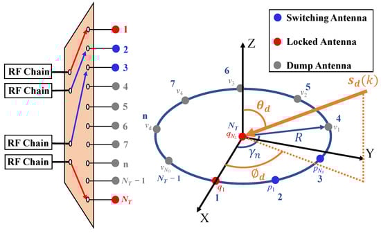
Figure 1.
System model.
- antennas are locked, which means these antennas are always connected to RF chains;
- () antennas are selected and connected to RF chains in each switching;
- The remaining () antennas are dumped, which means these antennas are not connected to the RF chain in each switching.
After () switchings, all antennas of the SUCA are selected.
The label set of the switching antennas in the -th switching is ; the label set of locked antennas in a SUCA is ; the dump antennas in the -th switching are labeled as . Thus, the label set of switching antennas in a SUCA can be expressed as
We try to recover the complete covariance matrix of the FUCA by jointly processing snapshots collected in each switching.
The -th snapshot in the -th switching can be written as
where denotes the arriving signals, and is the additive white Gaussian noise with zero mean and variance. The diagonal matrix represents the connections between the RF chains and antenna elements in the -th switching, defined as
Hence, the sample matrix received by the -th switching is written as
Afterwards, the L sample matrices are packed in which is given as
Notably, the simultaneously sampled snapshots are able to construct the sample covariance matrix. More specifically, each switching antenna collects only snapshots, but each locked antenna collects snapshots because the locked antenna is selected all the time. Consequently, the sample covariance matrix of the received data can be estimated as
For the purpose of illustrating the switching scheme clearly, the SUCA with antenna elements and RF chains connected to locked antennas and switching antennas is shown in Figure 2. We lock the center antenna together with the first antenna on the circle, and switchings are conducted. Thus, the structure of the covariance matrix in this switching scheme is plotted in Figure 3.
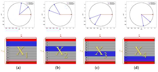
Figure 2.
Switching scheme: (a) the first switching; (b) the second switching; (c) the third switching; (d) the fourth switching.
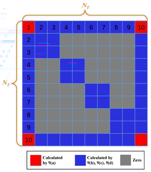
Figure 3.
Structure of .
Similarly, the -th snapshot received by the FUCA is written as
where . Moreover, the complete covariance matrix of the FUCA is calculated as
Additionally, the 2D-DOA estimation can be conducted with the classical MUSIC algorithm as follows
where and are the estimated signal subspace and noise subspace, respectively. Accordingly, the 2D spatial spectrum is formed as
We try to recover by retrieving the missing entries of . This is a tricky problem because the covariance matrix of UCA does not have the Toeplitz property.
3. Deep Feedforward Network for Covariance Matrix Completion
In this section, we design the label and input of the proposed DFN and discuss the network architecture and training strategy.
3.1. Data and DFN Architecture
To construct the input data , we use the real and imaginary parts of the upper triangular elements of the sample covariance matrix and arrange them into a real vector in terms of
where and denote the real part and the imaginary part of , respectively. The vectorization of the upper triangular part of is shown in Figure 4.
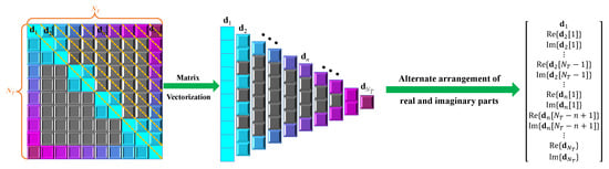
Figure 4.
Vectorization of the upper triangular part of .
Similarly, the label is a real vector obtained by the vectorization of the upper triangular part of according to (14).
Our goal is to design a DFN that can estimate the complete covariance matrix from . Given , the estimation of can be expressed as
where denotes the parameters of the network. The values of the parameters are learned via the offline training.
A sketch of the DFN architecture is shown in Figure 5. The DFN consists of one input layer, one output layer and some hidden layers. The main design considerations for network are to choose the depth of the network and the width of each layer. As a consequence, we choose a fully connected, feedforward network with = 5 hidden layers, and each hidden layer is composed of = 4096 neurons via experimentations guided by monitoring the estimation error. Moreover, each hidden layer consists of a fully connected (FC) layer and an active function.
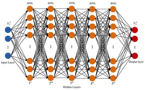
Figure 5.
Architecture of DFN.
In the -th FC layer, weights and biases are expressed by and , respectively. Furthermore, the output vector of the -th FC layer is defined as
where is the input vector of the -th FC layer.
Next, the output of the -th FC layer is sent into the active function. Owing to the nonlinearity of the active function, the DFN can fit arbitrary curves. We employ the Leaky rectified linear unit (LeakyReLU), which is defined as
where is a small constant. As a result, the output of the -th hidden layer can be expressed by
where is the input of the -th FC layer.
3.2. Training Strategy
The training setup of the DFN is illustrated in Figure 6. In the strategy, , and are the input vector, label vector and output vector of the DFN model, respectively.
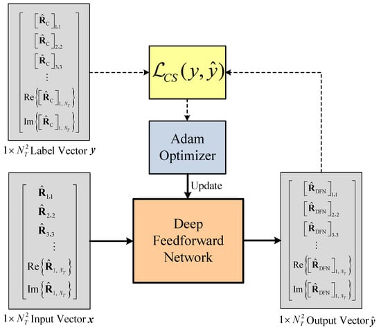
Figure 6.
Block diagram of the DFN training system.
The cosine similarity (CS) can better measure the similarity of two vectors. Therefore, the loss function is defined as
During training, is updated by an Adam optimizer that runs back propagation based on the loss function in (19). To improve training efficiency, the following techniques are employed. Training data are provided to the model in minibatches, which takes advantage of the high throughput of parallel processing in the graphics processing unit (GPU) and minimizes the latency of memory copying. The learning rate decays exponentially for fine-tuning as the training proceeds.
The training configurations for the DFN are listed in Table 1. A stochastic gradient descent (SGD)-based Adam optimizer is used. The learning rate is initially set to and decayed by in each epoch.

Table 1.
DFN hyperparameters.
4. Simulation Results
In this section, we conduct numerical experiments to validate the effectiveness of the SUMC estimator.
4.1. Simulation Conditions
The considered system consists of antennas in the form of UCA and RF chains. At each time instant, the switching network sequentially selects 4 antennas out of the 10 antennas according to Figure 2, where the UCA antenna elements are numbered counterclockwise, and the center element is marked as 10. In addition, the simulation parameters that are used to generate the training and test datasets are listed in Table 2.
Table 2.
Simulation parameters.
To evaluate the performance of the SUMC estimator for 2D-DOA estimation, the root mean square error (RMSE) is calculated by running Monte Carlo simulations. The RMSE is defined as
where is the total number of Monte Carlo simulations, and , , and are the actual elevation angle, actual azimuth angle, estimated elevation angle and estimated azimuth angle of the -th source in the -th Monte Carlo simulation, respectively. Moreover, and are obtained by a 2D spatial spectrum search scheme based on the classical MUSIC algorithm. Meanwhile, the direction of D sources are randomly generated from the two-dimensional angular space in each Monte Carlo simulation.
4.2. Network Architecture Analysis
In this section, we evaluate the performance of different FC networks for covariance matrix completion. Four datasets were generated in scenarios of 1, 2, 3 and 4, respectively. Each individual dataset contains 250,000 sample covariance matrices and corresponding 250,000 complete covariance matrices, of which 80% are used for training, and a subset of the remaining 20% is used for validation. The training data for all FC networks is a mixture of the four datasets. The evolution of the loss on the validation set in the training of different FC networks is shown in Figure 7. In the legend of Figure 7, the N-M represents the FC network with N hidden layers, and each hidden layer is composed of M neurons; moreover, 6-2048 × 2-4096 × 4 represents the FC network with six hidden layers. The first two hidden layers consist of 2048 neurons each, and the remaining hidden layers consist of 4096 neurons each.
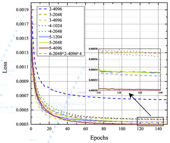
Figure 7.
Evolution of loss on the validation set in the training of different FC networks.
As shown in Figure 7, the training process starts with a fast fitting followed by a long fine-tuning phase. The loss decreases drastically in the first 40 epochs, then decreases slowly but steadily until hitting a floor. Obviously, the 5-4096 curve is the lowest, and the 2-4096 curve is the highest, indicating that properly expanding and deepening the network can improve its ability to estimate the complete covariance matrix. However, the 6-2048 × 2-4096 × 4 curve is higher than the 5-4096 curve. The main reasons for the performance degradation are gradient instability and network degradation issues in deep networks. Therefore, larger and deeper networks do not necessarily perform better, and the appropriate network needs to be selected according to the specific problem. For the covariance matrix completion problem in this paper, the optimal FC network contains five hidden layers, and each hidden layer consists of 4096 neurons.
Consequently, we trained two DFN models to perform covariance matrix completion in scenarios of 1, 2, 3, 4 and the scenario of D = 5, respectively.
4.3. Comparison to Fully Sampled UCA
In this section, we assess the performance of the SUMC algorithm in scenarios of 1, 2 and 3. Additionally, we consider the RMSE of the classical MUSIC algorithm applied to the FUCA, which we use as a lower bound. The RMSE of the classical MUSIC algorithm applied to the FUCA is labeled as FUCA; meanwhile, the RMSE of SUMC algorithm applied to a SUCA is labeled as SUCA.
Figure 8 and Figure 9 depict that the RMSE of the SUMC algorithm decreases considerably as SNR or increases in scenarios of 1, 2 and 3. Apparently, the SUCA curve gradually approaches the FUCA curve as SNR or increases. Nevertheless, there is a gap between the two curves, and the gap between the SUCA and FUCA curve is becoming wider as increases. Notably, the proposed algorithm performs worse than the MUSIC algorithm applied to the FUCA because the estimated covariance matrix in (15) is only an approximation of the complete covariance matrix in (11). In summary, the SUMC estimator can perform 2D-DOA estimation and provide reasonable performance.
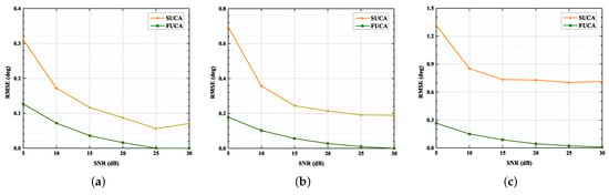
Figure 8.
RMSE versus SNR, = 1024: (a) ; (b) ; (c) .
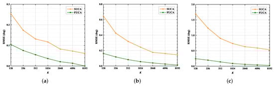
Figure 9.
RMSE versus , SNR = 15 dB: (a) ; (b) ; (c) .
4.4. Comparison to Partial Array
In this section, we compare the performance of the SUMC algorithm and classical MUSIC algorithm applied to a partial array (PA) in the scenario of 3. In addition, the layout of the PA is the same as in Figure 2a because a SUCA without matrix completion can use only four elements for DOA estimation. The performance of 2D-DOA estimation is evaluated by RMSE and Success Probability. A successful trial is defined as follows:
- The number of peaks searched by 2D spatial spectrum search scheme is equal to ;
- The divation of each DOA estimate satisfies
Therefore, the Success Probability is expressed as
where is the number of successful trials in each simulation scenario.
As shown in Figure 10a, the estimation accuracy of the three methods is improved as SNR increases, and the RMSE of the proposed method is significantly smaller than that of the MUSIC algorithm applied to PA under low and moderate SNRs. As shown in Figure 10b, it is apparent that the PA curve is far below the SUCA curve. Moreover, the PA curve is always below , and both the SUCA curve and the FUCA curve are almost when SNR ranges from 5 dB to 30 dB. As a result, the effective aperture of the SUCA is enlarged by the SUMC algorithm; meanwhile, the accuracy of DOA estimation is improved.
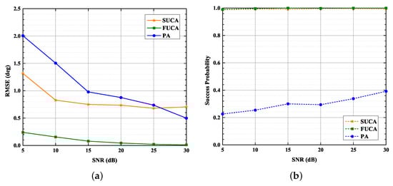
Figure 10.
RMSE, Success Probability versus SNR, , : (a) RMSE versus SNR; (b) Success Probability versus SNR.
4.5. Resolution of 2D-DOA Estimation
In this section, we evaluate the resolution of the proposed algorithm and the MUSIC algorithm performed in PA when SNR is set to 10 dB and is set to 1024. The DOAs of two sources in each Monte Carlo trial are selected as follows:
- The total angular separation of two sources is defined as
- The is randomly selected from , is then calculated by
- The DOA of the first source is randomly selected from the two-dimensional angular space
- The DOA of the second source is then given by
The RMSE for DOAs and the Success Probability for DOA estimation are shown in Figure 11a,b, respectively. As detailed in Figure 11a, for as high as , SUCA has an RMSE smaller than , whereas PA has an RMSE larger than ; moreover, the difference between the PA and the SUCA is most significant at low . Figure 11b displays that the Success Probability of the SUCA reaches when ; however, the Success Probability of PA is less than when . The results in Figure 11 indicate that the SUMC estimator provides better resolution.
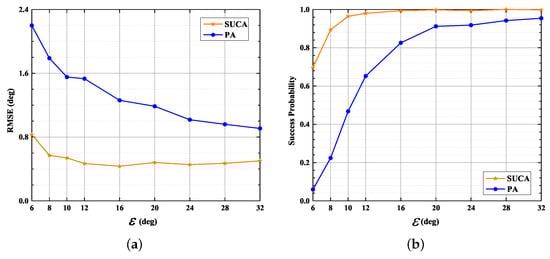
Figure 11.
RMSE, Success Probability versus , = 1024, SNR = 10 dB: (a) RMSE versus ; (b) Success Probability versus .
4.6. Underdetermined 2D-DOA Estimation Problem
In this section, we focus on the capability of the SUMC estimator to solve the underdetermined 2D-DOA estimation problem where . D is set to four and five as . The RMSE in scenarios of four sources and five sources are displayed in Figure 12 and Figure 13, respectively.
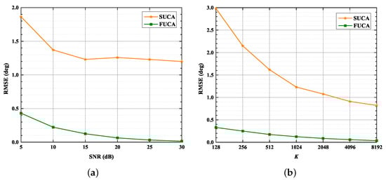
Figure 12.
RMSE versus SNR, : = 4. (a) RMSE versus SNR, ; (b) RMSE versus , SNR = 15 dB.
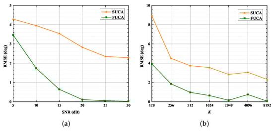
Figure 13.
RMSE versus SNR, . = 5: (a) RMSE versus SNR, ; (b) RMSE versus , SNR = 15 dB.
As shown in Figure 12 and Figure 13, the performance of the SUMC estimator improves considerably as SNR or increases in scenarios of four and five sources. In addition, it should be noted from Figure 12 that the RMSE of DOAs in the SUCA approaches that in the FUCA under large . In detail, Figure 13 depicts that the RMSE of the proposed algorithm is lower than in the scenario of five sources when SNR > 20 dB and .
Moreover, the spatial spectra obtained from the SUMC estimator are depicted in Figure 14 and Figure 15, where the red circles represent the ground truth value of DOAs. The SNR and are fixed at 15 dB and 1024, respectively. Figure 14 shows four high and sharp peaks. Significantly, there is almost no deviation between the four peaks and the four red circles. It can be seen from Figure 15 that five peaks have been found by the SUMC estimator; yet there is a slight deviation between the five peaks and the five red circles. On the whole, the proposed algorithm can deal with the underdetermined 2D-DOA estimation problem with acceptable performance under moderate SNR and .
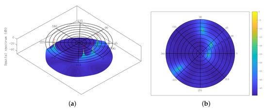
Figure 14.
Spatial spectrum using SUMC estimator for solving four sources, SNR = 15 dB, : (a) front; (b) top.
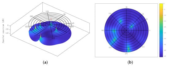
Figure 15.
Spatial spectrum using SUMC estimator for solving five sources, SNR = 15 dB, : (a) front; (b) top.
5. Conclusions
In this paper, a 2D-DOA estimation scheme based on covariance matrix completion in a SUCA is proposed. The proposed algorithm starts by using a DFN to complete the sample covariance matrix of a SUCA; then the MUSIC algorithm is performed with the completed covariance matrix. The simulation results indicate that the SUMC estimator enlarges the effective aperture of a SUCA; thereby improving the accuracy, resolution and success probability of 2D-DOA estimation in a SUCA. Furthermore, the results show that the proposed algorithm is able to handle the underdetermined 2D-DOA estimation problem with reasonable performance.
Author Contributions
Conceptualization, R.M., Y.T., Y.H. and Z.W.; methodology, R.M., Y.T., Y.H. and Z.W.; software, R.M. and Y.T.; validation, R.M. and Y.T.; formal analysis, R.M., Y.T. and Z.W.; writing—review and editing, R.M., Y.T. and Y.H.; visualization, R.M. and Z.W. All authors have read and agreed to the published version of the manuscript.
Funding
This research was funded by the Strategic Priority Research Program of the Chinese Academy of Sciences (Class A) (Subject Number: XDA153501, Sub-Subject Number: XDA15350103).
Institutional Review Board Statement
Not applicable.
Informed Consent Statement
Not applicable.
Data Availability Statement
Not applicable.
Conflicts of Interest
The authors declare no conflict of interest.
Abbreviations
The following abbreviations are used in this manuscript:
| 2D-DOA | Two-Dimensional Direction of Arrival |
| UCA | Uniform Circular Array |
| SUCA | Switching Uniform Circular Array |
| FUCA | Fully Sampled UCA |
| PA | Partial Array |
| SLA | Sparse Linear Array |
| RF | Radio Frequency |
| DOFs | Degrees of Freedom |
| MUSIC | Multiple Signal Classification |
| ESPRIT | Estimation of Signal Parameters via Rotational Invariance |
| GSDC | Generalized Sum and Difference Coarray |
| SNACD | Sparse Nested Arrays with Coprime Displacement |
| SIMC | Shift-Invariant Matrix Completion |
| NSCA | Nested Sparse Circular Array |
| DL | Deep Learning |
| NN | Neural Network |
| CNN | Convolutional Neural Network |
| DFN | Deep Feedforward Network |
| SUMC | Switching UCA Matrix Completion |
| LeakyReLU | Leaky Rectified Linear Unit |
| CS | Cosine Similarity |
| GPU | Graphics Processing Unit |
| SGD | Stochastic Gradient Descent |
References
- Bozorgasl, Z.; Dehghani, M.J. 2-D DOA estimation in wireless location system via sparse representation. In Proceedings of the 2014 4th International Conference on Computer and Knowledge Engineering (ICCKE), Mashhad, Iran, 29–30 October 2014; pp. 86–89. [Google Scholar] [CrossRef]
- Mirza, H.A.; Raja, M.A.Z.; Chaudhary, N.I.; Qureshi, I.M.; Malik, A.N. A Robust Multi Sample Compressive Sensing Technique for DOA Estimation Using Sparse Antenna Array. IEEE Access 2020, 8, 140848–140861. [Google Scholar] [CrossRef]
- Wen, F.; Shi, J.; Zhang, Z. Joint 2D-DOD, 2D-DOA, and Polarization Angles Estimation for Bistatic EMVS-MIMO Radar via PARAFAC Analysis. IEEE Trans. Veh. Technol. 2020, 69, 1626–1638. [Google Scholar] [CrossRef]
- Wu, Y.; Chen, H.; Chen, Y. A method of 2-D DOA estimation of coherent signals based on uniform circular array via spatial smoothing. In Proceedings of the 2011 IEEE CIE International Conference on Radar, Chengdu, China, 24–27 October 2011; Volume 1, pp. 312–314. [Google Scholar] [CrossRef]
- Xu, K.; Quan, Y.; Bie, B.; Xing, M.; Nie, W.; E, H. Fast Direction of Arrival Estimation for Uniform Circular Arrays With a Virtual Signal Subspace. IEEE Trans. Aerosp. Electron. Syst. 2021, 57, 1731–1741. [Google Scholar] [CrossRef]
- Mathews, C.; Zoltowski, M. Eigenstructure techniques for 2-D angle estimation with uniform circular arrays. IEEE Trans. Signal Process. 1994, 42, 2395–2407. [Google Scholar] [CrossRef]
- Pesavento, M.; Bohme, J. Direction of arrival estimation in uniform circular arrays composed of directional elements. In Proceedings of the Sensor Array and Multichannel Signal Processing Workshop Proceedings, Rosslyn, VA, USA, 6 August 2002; pp. 503–507. [Google Scholar] [CrossRef]
- Pal, P.; Vaidyanathan, P.P. Coprime sampling and the music algorithm. In Proceedings of the 2011 Digital Signal Processing and Signal Processing Education Meeting (DSP/SPE), Sedona, AZ, USA, 4–7 January 2011; pp. 289–294. [Google Scholar] [CrossRef]
- Shi, Z.; Zhou, C.; Gu, Y.; Goodman, N.A.; Qu, F. Source Estimation Using Coprime Array: A Sparse Reconstruction Perspective. IEEE Sens. J. 2017, 17, 755–765. [Google Scholar] [CrossRef]
- Pal, P.; Vaidyanathan, P.P. Nested Arrays: A Novel Approach to Array Processing With Enhanced Degrees of Freedom. IEEE Trans. Signal Process. 2010, 58, 4167–4181. [Google Scholar] [CrossRef] [Green Version]
- Vaidyanathan, P.P.; Pal, P. Sparse Sensing With Co-Prime Samplers and Arrays. IEEE Trans. Signal Process. 2011, 59, 573–586. [Google Scholar] [CrossRef]
- Shi, J.; Hu, G.; Zhang, X.; Sun, F.; Zheng, W.; Xiao, Y. Generalized Co-Prime MIMO Radar for DOA Estimation With Enhanced Degrees of Freedom. IEEE Sens. J. 2018, 18, 1203–1212. [Google Scholar] [CrossRef]
- Basikolo, T.; Ichige, K.; Arai, H. A Novel Mutual Coupling Compensation Method for Underdetermined Direction of Arrival Estimation in Nested Sparse Circular Arrays. IEEE Trans. Antennas Propag. 2018, 66, 909–917. [Google Scholar] [CrossRef]
- Li, J.; He, Y.; Ma, P.; Zhang, X.; Wu, Q. Direction of Arrival Estimation Using Sparse Nested Arrays With Coprime Displacement. IEEE Sens. J. 2021, 21, 5282–5291. [Google Scholar] [CrossRef]
- Lee, J.H.; Woo, J.M. Interferometer Direction-Finding System With Improved DF Accuracy Using Two Different Array Configurations. IEEE Antennas Wirel. Propag. Lett. 2015, 14, 719–722. [Google Scholar] [CrossRef]
- Moghaddasi, J.; Wu, K. Millimeter-Wave Multifunction Multiport Interferometric Receiver for Future Wireless Systems. IEEE Trans. Microw. Theory Tech. 2018, 66, 1452–1466. [Google Scholar] [CrossRef]
- Doi, Y.; Ichige, K.; Arari, H.; Matsuno, H.; Nakano, M. Antenna switching based on the relation between the relative location of array elements for high resolution 2-D DOA estimation. In Proceedings of the 2014 6th International Symposium on Communications, Control and Signal Processing (ISCCSP), Athens, Greece, 21–23 May 2014; pp. 437–440. [Google Scholar] [CrossRef]
- Wu, W.; Cooper, C.C.; Goodman, N.A. Switched-Element Direction Finding. IEEE Trans. Aerosp. Electron. Syst. 2009, 45, 1209–1217. [Google Scholar] [CrossRef]
- Garg, V.; Giménez-Febrer, P.; Pagès-Zamora, A.; Santamaria, I. DOA Estimation via Shift-Invariant Matrix Completion. Signal Process. 2021, 183, 107993. [Google Scholar] [CrossRef]
- Jiang, G.; Mao, X.P.; Liu, Y.T. Underdetermined DOA Estimation via Covariance Matrix Completion for Nested Sparse Circular Array in Nonuniform Noise. IEEE Signal Process. Lett. 2020, 27, 1824–1828. [Google Scholar] [CrossRef]
- Cong, J.; Wang, X.; Huang, M.; Wan, L. Robust DOA Estimation Method for MIMO Radar via Deep Neural Networks. IEEE Sens. J. 2021, 21, 7498–7507. [Google Scholar] [CrossRef]
- Liu, Z.M.; Zhang, C.; Yu, P.S. Direction-of-Arrival Estimation Based on Deep Neural Networks With Robustness to Array Imperfections. IEEE Trans. Antennas Propag. 2018, 66, 7315–7327. [Google Scholar] [CrossRef]
- Yao, Y.; Lei, H.; He, W. A-CRNN-Based Method for Coherent DOA Estimation with Unknown Source Number. Sensors 2020, 20, 2296. [Google Scholar] [CrossRef] [Green Version]
- Perotin, L.; Serizel, R.; Vincent, E.; Guérin, A. CRNN-Based Multiple DoA Estimation Using Acoustic Intensity Features for Ambisonics Recordings. IEEE J. Sel. Top. Signal Process. 2019, 13, 22–33. [Google Scholar] [CrossRef] [Green Version]
- Ozanich, E.; Gerstoft, P.; Niu, H. A feedforward neural network for direction-of-arrival estimation. J. Acoust. Soc. Am. 2020, 147, 2035–2048. [Google Scholar] [CrossRef]
- Zhu, W.; Zhang, M.; Li, P.; Wu, C. Two-Dimensional DOA Estimation via Deep Ensemble Learning. IEEE Access 2020, 8, 124544–124552. [Google Scholar] [CrossRef]
- Barthelme, A.; Utschick, W. DoA Estimation Using Neural Network-Based Covariance Matrix Reconstruction. IEEE Signal Process. Lett. 2021, 28, 783–787. [Google Scholar] [CrossRef]
Publisher’s Note: MDPI stays neutral with regard to jurisdictional claims in published maps and institutional affiliations. |
© 2022 by the authors. Licensee MDPI, Basel, Switzerland. This article is an open access article distributed under the terms and conditions of the Creative Commons Attribution (CC BY) license (https://creativecommons.org/licenses/by/4.0/).