
Robust PMBM Filter with Unknown Detection Probability Based on Feature Estimation


Abstract
:1. Introduction
2. Background
2.1. PMBM RFS Density
2.2. PMBM Filter
2.3. Gamma Distribution and Inverse Gamma Distribution
3. The Proposed Robust Filter with Unknown Detection Probability
3.1. Target State Model and Observation Model
3.2. The Implementtation of Proposed Algorithm
| Algorithm 1 Description of the proposed robust filter |
| Input: |
| Output: |
| Prediction process: |
| Poisson process: see Formula (32) |
| MBM process: |
| for jth global hypothesis do |
| for ith Bernoulli in the jth global hypothesis do |
| see Formulas (36)–(38) |
| end for |
| end for |
| Update process: |
| Poisson process: see Formula (41) |
| MBM process: |
| If the target is the first detected |
| for each measurement do |
| Formulas (42) and (43) |
| end for |
| If the target detected before |
| for ith Bernoulli in the jth global hypothesis do |
| Formulas (52)–(54) |
| end for |
| Construct global hypothesis: Gibbs sampler |
| Estimate target state and detection probability |
| Pruning and Merging |
3.3. The Computation Complexity of the Proposed Algorithm
4. Simulation Setup and Results
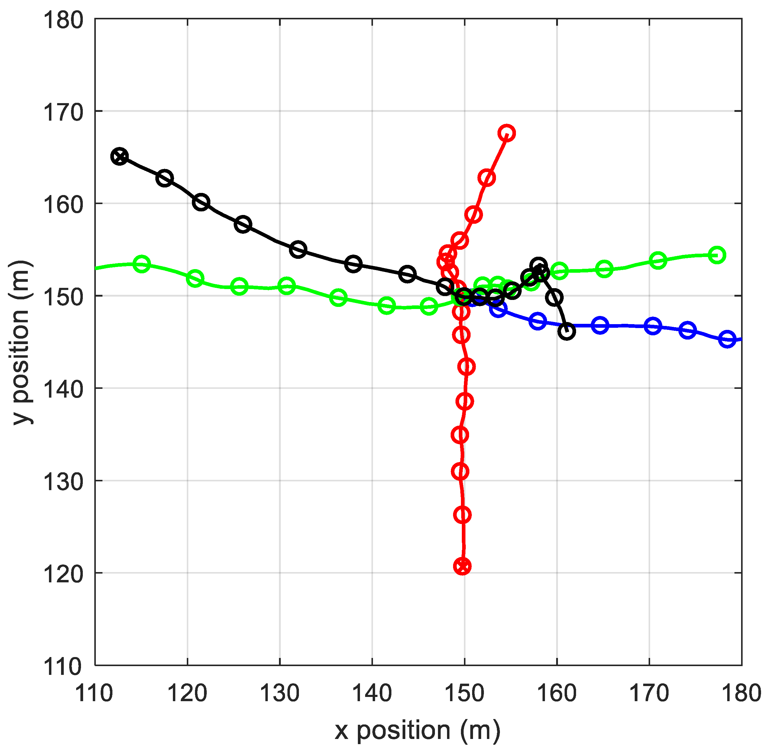
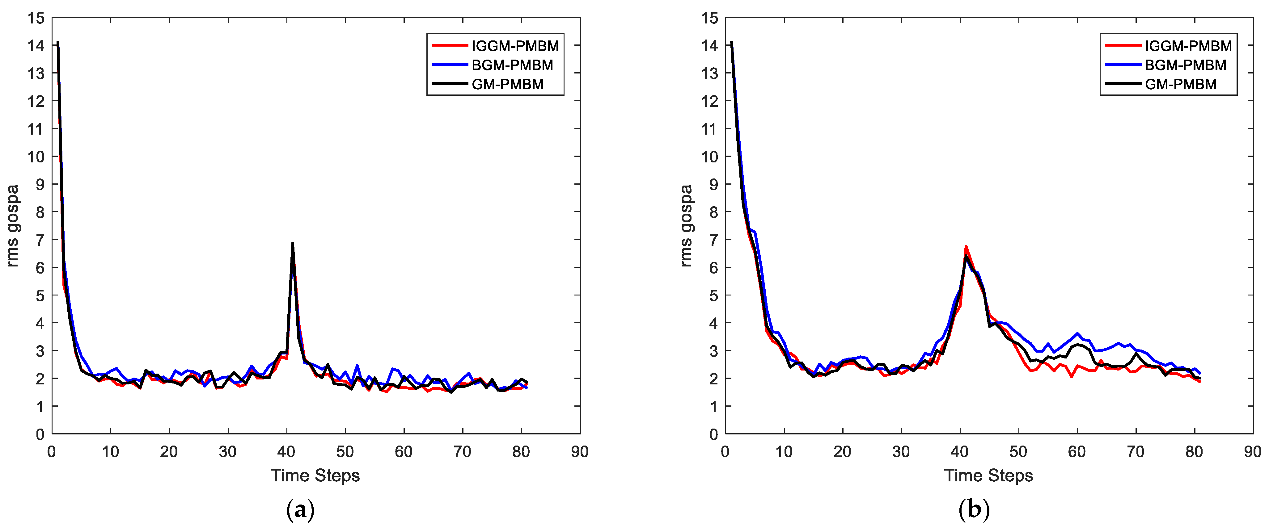
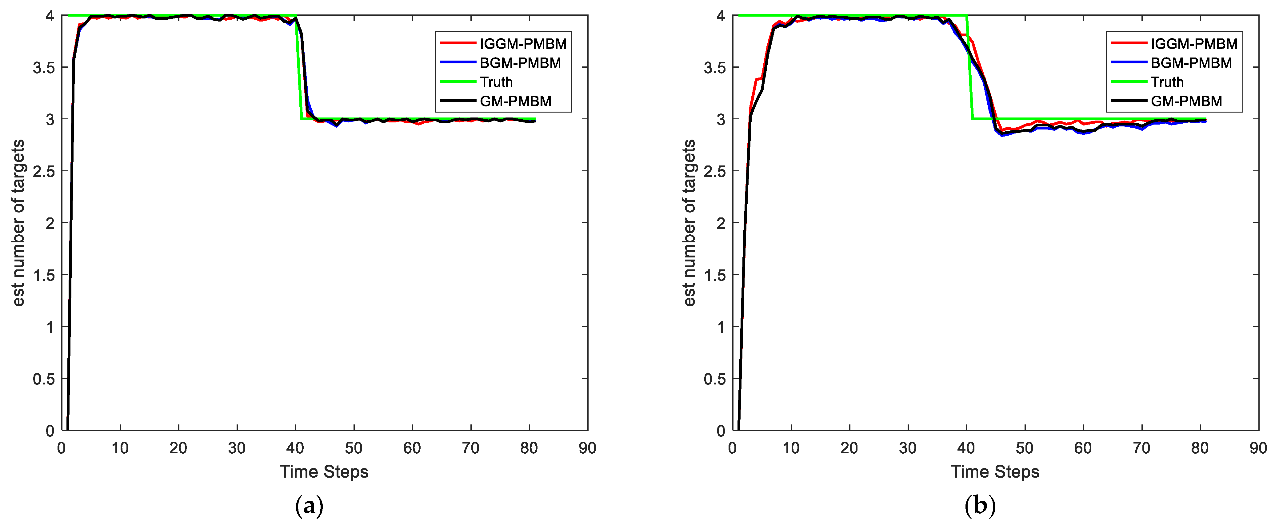
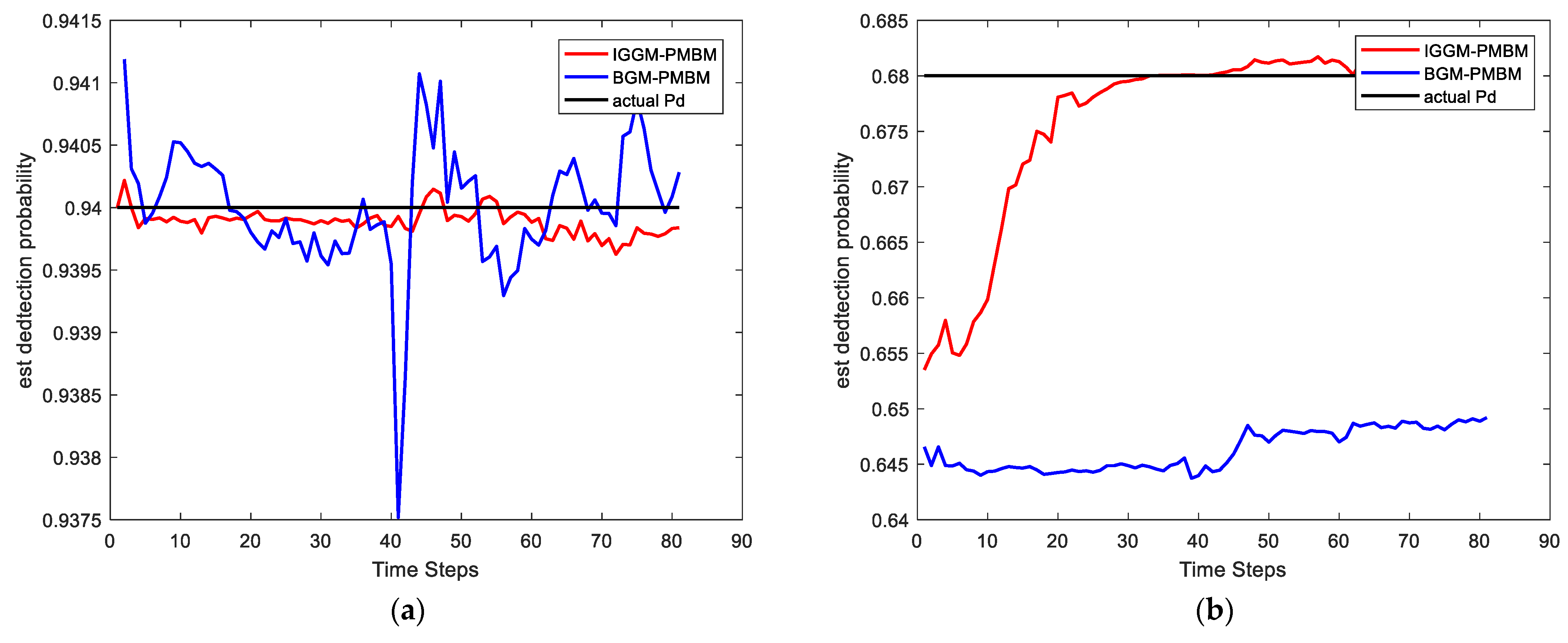
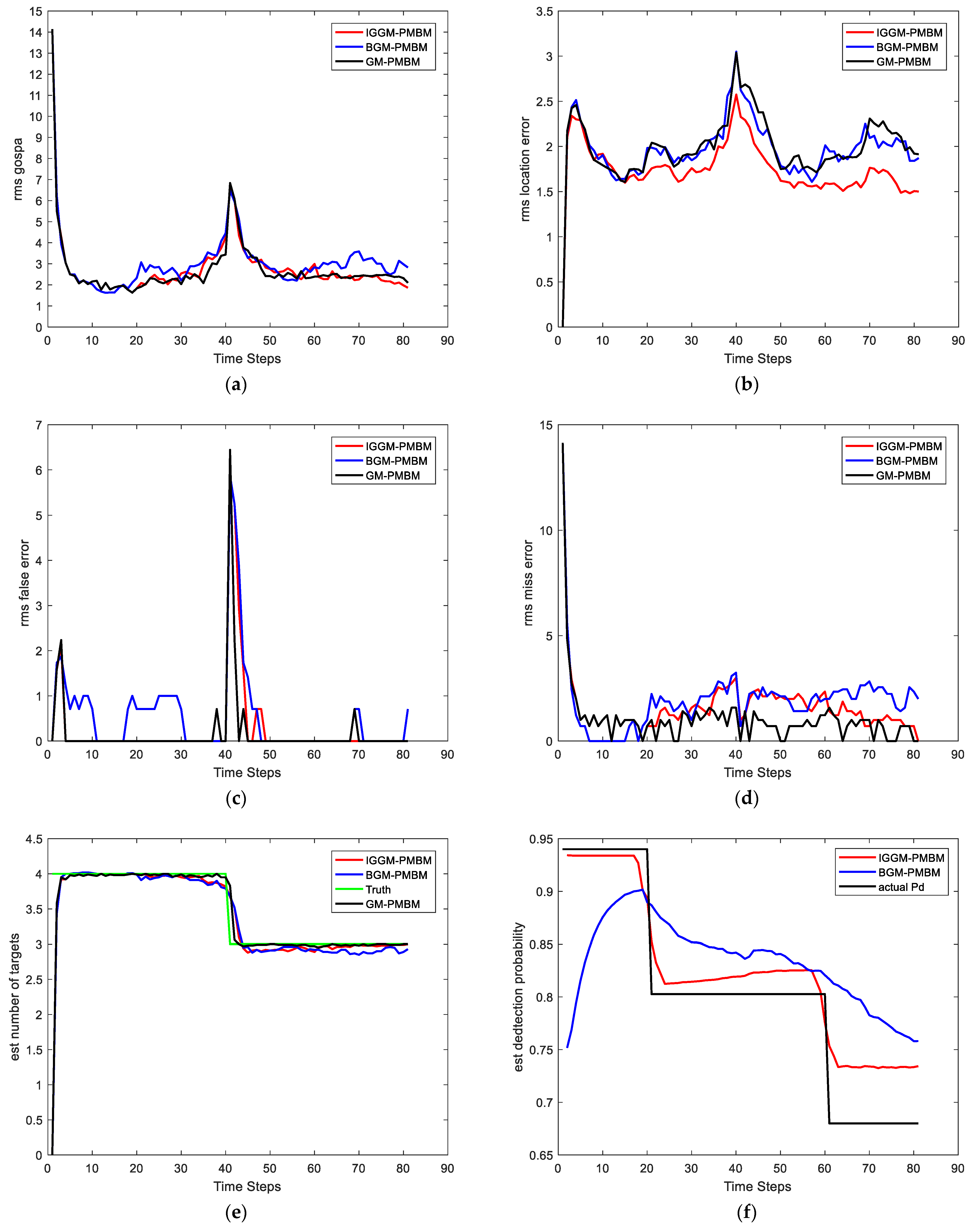
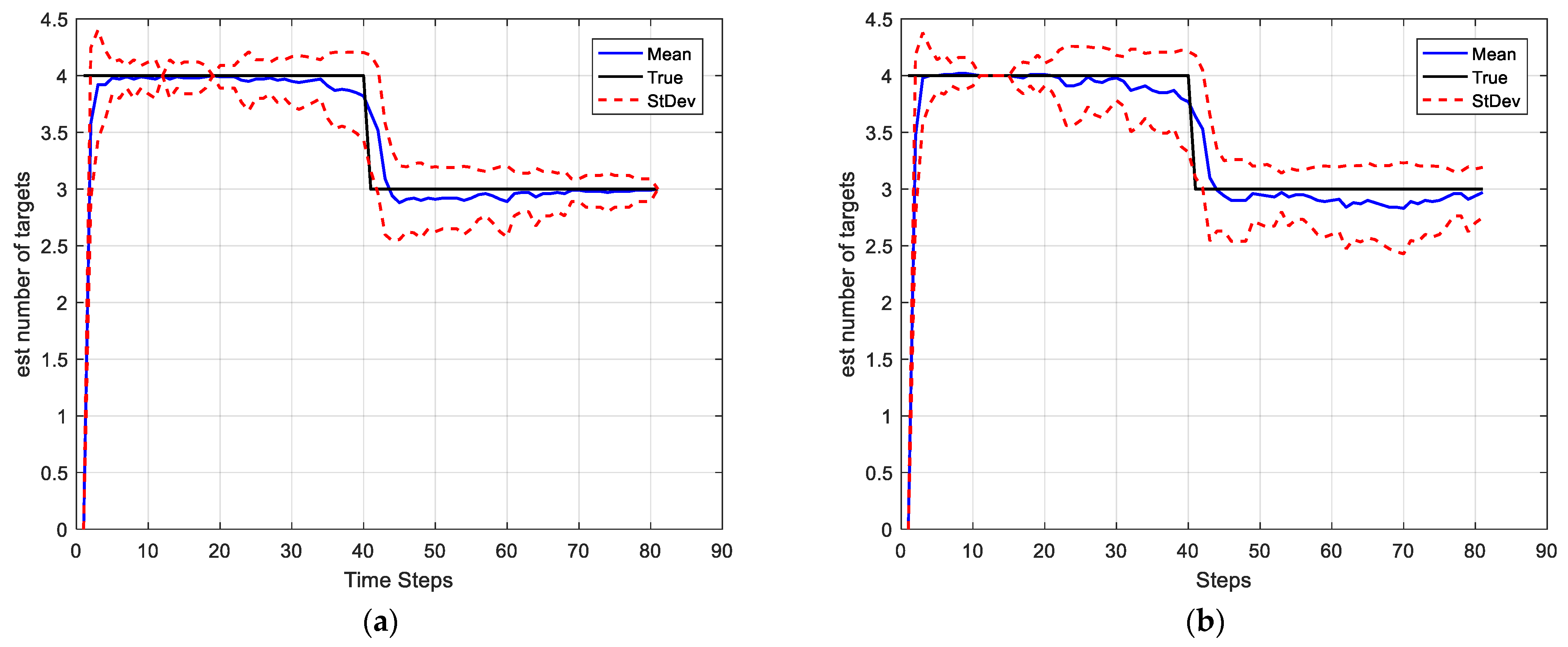
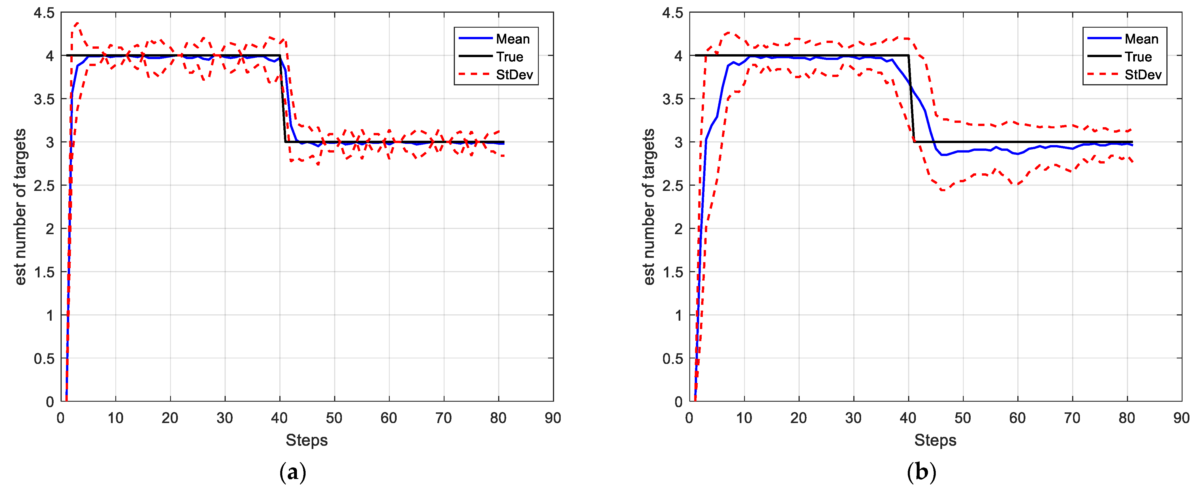
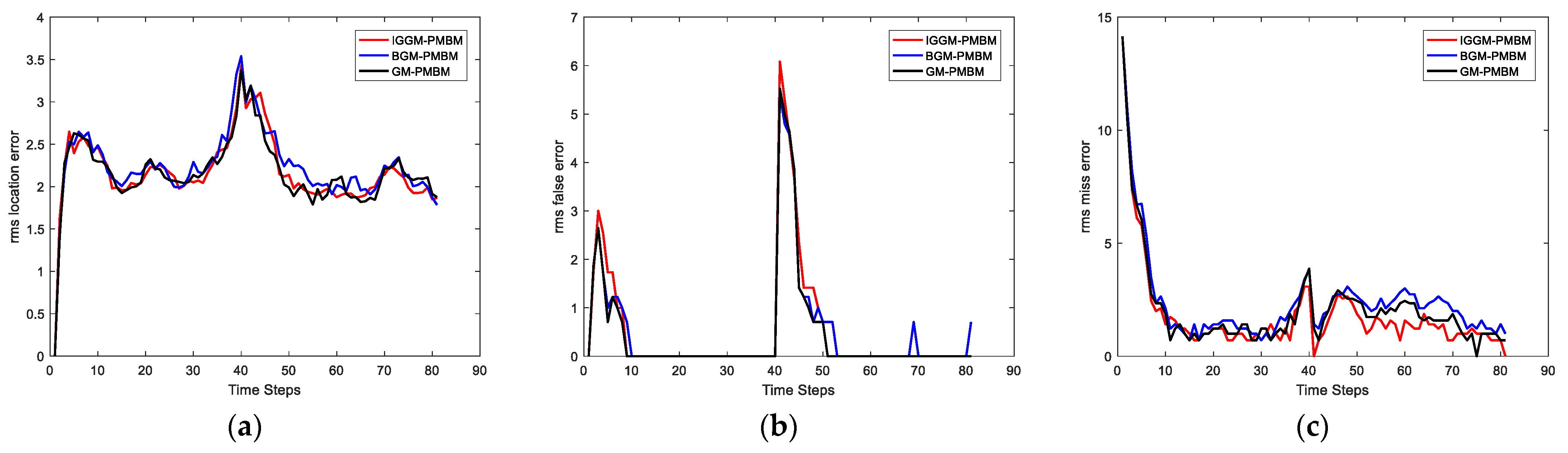
4.1. Simulation Scenario 1
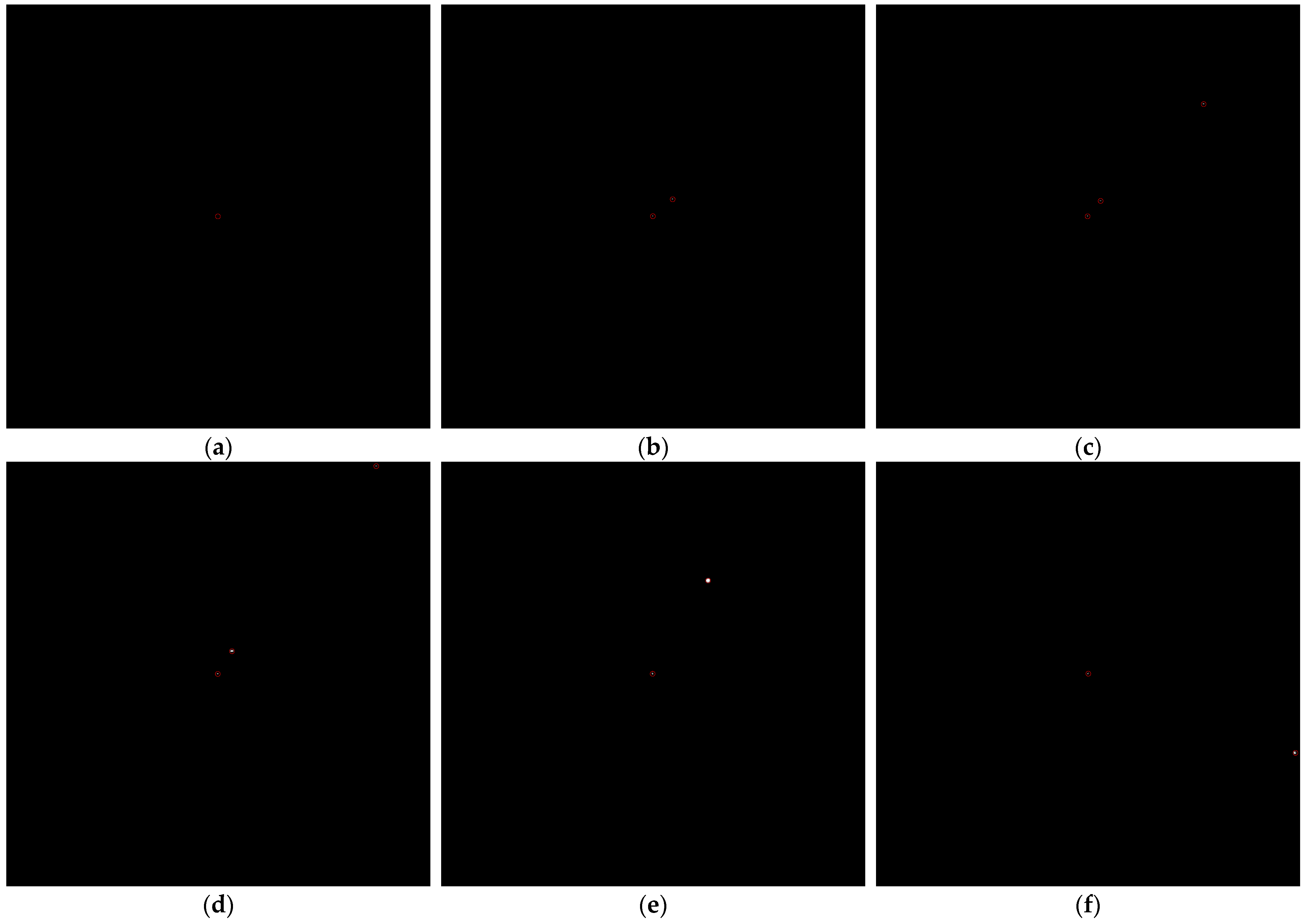
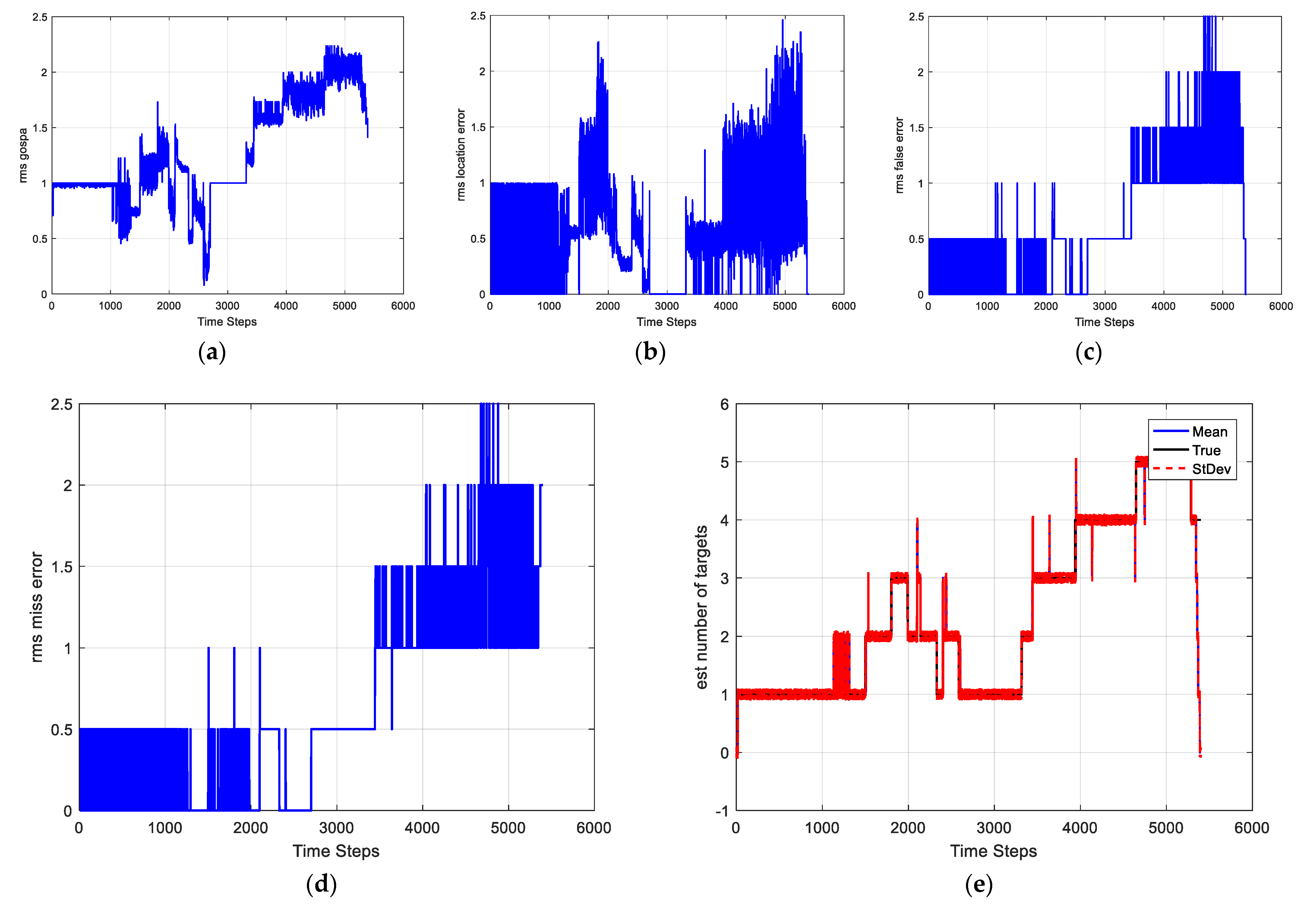
4.2. Simulation Scenario 2
5. Conclusions
Author Contributions
Funding
Institutional Review Board Statement
Informed Consent Statement
Data Availability Statement
Conflicts of Interest
References
- Vo, B.-N.; Mallick, M.; Bar-Shalom, Y.; Coraluppi, S.; Osborne, R.; Mahler, R.; Vo, B.-T. Multitarget tracking. Wiley Encycl. Electr. Electron. Eng. 2015, 2015. [Google Scholar]
- Bohnsack, E.; Lilja, A. Multi-Object Tracking Using Either End-to-End Deep Learning or PMBM Filtering. Master’s Thesis, Chalmers University Oftechnology, Gothenburg, Sweden, 2019. [Google Scholar]
- Bouraya, S., Jr.; Belangour, A. Multi object tracking: A survey. In Proceedings of the Thirteenth International Conference on Digital Image Processing (ICDIP 2021), Singapore, 20–23 May 2021; International Society for Optics and Photonics: Bellingham, DC, USA, 2021; p. 118780. [Google Scholar]
- Pang, S.; Radha, H. Multi-Object Tracking using Poisson Multi-Bernoulli Mixture Filtering for Autonomous Vehicles. In Proceedings of the ICASSP 2021–2021 IEEE International Conference on Acoustics, Speech and Signal Processing (ICASSP), Toronto, ON, Canada, 6–11 June 2021; IEEE: Piscataway, NJ, USA, 2021; pp. 7963–7967. [Google Scholar]
- Rezatofighi, S.H.; Gould, S.; Vo, B.T.; Vo, B.-N.; Mele, K.; Hartley, R. Multi-target tracking with time-varying clutter rate and detection profile: Application to time-lapse cell microscopy sequences. IEEE Trans. Med. Imaging 2015, 34, 1336–1348. [Google Scholar] [CrossRef] [Green Version]
- Mahler, R.P. Statistical Multisource-Multitarget Information Fusion; Artech House, Inc.: Norwood, MA, USA, 2007. [Google Scholar]
- Mahler, R.P. Advances in Statistical Multisource-Multitarget Information Fusion; Artech House, Inc.: Norwood, MA, USA, 2014. [Google Scholar]
- Blackman, S.S. Multiple hypothesis tracking for multiple target tracking. IEEE Aerosp. Electron. Syst. Mag. 2004, 19, 5–18. [Google Scholar] [CrossRef]
- Sathyan, T.; Chin, T.-J.; Arulampalam, S.; Suter, D. A multiple hypothesis tracker for multitarget tracking with multiple simultaneous measurements. IEEE J. Sel. Top. Signal Processing 2013, 7, 448–460. [Google Scholar] [CrossRef]
- Musicki, D.; Evans, R. Joint integrated probabilistic data association: JIPDA. IEEE Trans. Aerosp. 2004, 40, 1093–1099. [Google Scholar] [CrossRef]
- Mahler, R.P. Multitarget Bayes filtering via first-order multitarget moments. IEEE Trans. Aerosp. 2003, 39, 1152–1178. [Google Scholar] [CrossRef]
- Mahler, R. PHD filters of higher order in target number. IEEE Trans. Aerosp. 2007, 43, 1523–1543. [Google Scholar] [CrossRef]
- Reuter, S.; Vo, B.-T.; Vo, B.-N.; Dietmayer, K. The labeled multi-Bernoulli filter. IEEE Trans. Signal Processing 2014, 62, 3246–3260. [Google Scholar] [CrossRef]
- Vo, B.-N.; Vo, B.-T.; Phung, D. Labeled random finite sets and the Bayes multi-target tracking filter. IEEE Trans. Signal Processing 2014, 62, 6554–6567. [Google Scholar] [CrossRef] [Green Version]
- Vo, B.-T.; Vo, B.-N. Labeled random finite sets and multi-object conjugate priors. IEEE Trans. Signal Processing 2013, 61, 3460–3475. [Google Scholar] [CrossRef]
- García-Fernández, Á.F.; Williams, J.L.; Granström, K.; Svensson, L. Poisson multi-Bernoulli mixture filter: Direct derivation and implementation. IEEE Trans. Aerosp. 2018, 54, 1883–1901. [Google Scholar] [CrossRef] [Green Version]
- Xia, Y.; Granstrcom, K.; Svensson, L.; García-Fernández, Á.F. Performance Evaluation of Multi-Bernoulli Conjugate Priors for Multi-Target Filtering. In Proceedings of the 2017 20th International Conference on Information Fusion (Fusion), Xi’an, China, 10–13 July 2017; IEEE: Piscataway, NJ, USA, 2017; pp. 1–8. [Google Scholar]
- Mahler, R.; El-Fallah, A. CPHD filtering with unknown probability of detection. In Signal Processing, Sensor Fusion, and Target Recognition XIX, 2010, Proceedings of the International Society for Optics and Photonics, Guwahati, India, 11–15 December 2010; SPIE: Orlando, FL, USA, 2010; p. 76970. [Google Scholar]
- Mahler, R.P.; Vo, B.-T.; Vo, B.-N. CPHD filtering with unknown clutter rate and detection profile. IEEE Trans. Signal Processing 2011, 59, 3497–3513. [Google Scholar] [CrossRef]
- Vo, B.-T.; Vo, B.-N.; Hoseinnezhad, R.; Mahler, R.P. Robust multi-Bernoulli filtering. IEEE Trans. Signal Processing 2013, 7, 399–409. [Google Scholar] [CrossRef]
- Vo, B.T.; Vo, B.N.; Hoseinnezhad, R.; Mahler, R.P. Multi-Bernoulli filtering with unknown clutter intensity and sensor field-of-view. In Proceedings of the 2011 45th Annual Conference on Information Sciences and Systems, Baltimore, MD, USA, 23–25 March 2011; IEEE: Piscataway, NJ, USA, 2011; pp. 1–6. [Google Scholar]
- Punchihewa, Y.G.; Vo, B.-T.; Vo, B.-N.; Kim, D.Y. Multiple object tracking in unknown backgrounds with labeled random finite sets. IEEE Trans. Signal Processing 2018, 66, 3040–3055. [Google Scholar] [CrossRef] [Green Version]
- Li, G.; Kong, L.; Yi, W.; Li, X. Robust Poisson Multi-Bernoulli Mixture Filter With Unknown Detection Probability. IEEE Trans. Veh. Technol. 2020, 70, 886–899. [Google Scholar] [CrossRef]
- Ren, X.Y. A Novel Multiple Target Tracking Algorithm and Its Evaluation. Master’s Thesis, Graduate University of Chinese Academy of Sciences, Beijing, China, 2012. [Google Scholar]
- Li, C.; Wang, W.; Kirubarajan, T.; Sun, J.; Lei, P. PHD and CPHD filtering with unknown detection probability. IEEE Trans. Signal Processing 2018, 66, 3784–3798. [Google Scholar] [CrossRef]
- Clark, D.; Ristic, B.; Vo, B.-N.; Vo, B.T. Bayesian multi-object filtering with amplitude feature likelihood for unknown object SNR. IEEE Trans. Signal Processing 2009, 58, 26–37. [Google Scholar] [CrossRef]
- Qian, K.; Zhou, H.; Qin, H.; Rong, S.; Zhao, D.; Du, J. Guided filter and convolutional network based tracking for infrared dim moving target. Infrared Phys. Technol. 2017, 85, 431–442. [Google Scholar] [CrossRef]
- Zhang, Z.; Li, Q.; Sun, J. Multisensor RFS Filters for Unknown and Changing Detection Probability. Electronics 2019, 8, 741. [Google Scholar] [CrossRef] [Green Version]
- Vo, B.-N.; Vo, B.-T.; Hoang, H.G. An efficient implementation of the generalized labeled multi-Bernoulli filter. IEEE Trans. Signal Processing 2016, 65, 1975–1987. [Google Scholar] [CrossRef] [Green Version]
- Fatemi, M.; Granström, K.; Svensson, L.; Ruiz, F.J.; Hammarstrand, L. Poisson multi-Bernoulli mapping using Gibbs sampling. IEEE Trans. Signal Processing 2017, 65, 2814–2827. [Google Scholar] [CrossRef] [Green Version]
- Si, W.; Zhu, H.; Qu, Z. Robust Poisson multi-Bernoulli filter with unknown clutter rate. IEEE Access 2019, 7, 117871–117882. [Google Scholar] [CrossRef]
- Zhenzhen, S.; Hongbing, J.; Zhang, Y. A Poisson multi-Bernoulli mixture filter with spawning based on Kullback–Leibler divergence minimization. Chin. J. Aeronaut. 2021, 34, 154–168. [Google Scholar] [CrossRef]
- Granström, K.; Fatemi, M.; Svensson, L. Poisson multi-Bernoulli mixture conjugate prior for multiple extended target filtering. IEEE Trans. Aerosp. Electron. Syst. 2019, 56, 208–225. [Google Scholar] [CrossRef] [Green Version]
- Rahmathullah, A.S.; García-Fernández, Á.F.; Svensson, L. Generalized optimal sub-pattern assignment metric. In Proceedings of the 2017 20th International Conference on Information Fusion (Fusion), Xi’an, China, 10–13 July 2017; IEEE: Piscataway, NJ, USA, 2017; pp. 1–8. [Google Scholar]


| parameter | ||||||||
| value | 0.9 | 10 | 0.99 | 51 | 500 | 31 | 280 | 10 |
| (PD, λκ) | Proposed IGGM-PMBM | GM-PMBM | BGM-PMBM | |||||||||
|---|---|---|---|---|---|---|---|---|---|---|---|---|
| GOSPA | LE | ME | FE | GOSPA | LE | ME | FE | GOSPA | LE | ME | FE | |
| (0.94, 10) | 2.7477 | 1.7745 | 1.9277 | 0.8278 | 2.7511 | 1.7780 | 1.9277 | 0.8315 | 2.7592 | 1.7767 | 1.9181 | 0.8819 |
| (0.94, 15) | 2.8097 | 1.7897 | 1.9798 | 0.8784 | 2.7940 | 1.7876 | 1.9689 | 0.8571 | 2.7963 | 1.7895 | 1.9563 | 0.8889 |
| (0.94, 20) | 2.8417 | 1.7886 | 2.0154 | 0.9027 | 2.8534 | 1.7985 | 1.9985 | 0.9558 | 2.8538 | 1.7990 | 1.9783 | 0.9969 |
| (0.94, 25) | 2.8730 | 1.7937 | 2.0215 | 0.9750 | 2.9012 | 1.8063 | 2.0846 | 0.8992 | 2.9098 | 1.8098 | 2.0638 | 0.9655 |
| (0.68, 10) | 3.7648 | 2.2141 | 2.7499 | 1.3076 | 3.8460 | 2.2045 | 2.9187 | 1.1889 | 3.9832 | 2.2184 | 3.0123 | 1.3676 |
| (0.68, 15) | 4.0033 | 2.2626 | 3.0358 | 1.3005 | 3.9756 | 2.2422 | 3.0358 | 1.2497 | 4.1448 | 2.2610 | 3.1456 | 1.3494 |
| (0.68, 20) | 4.1351 | 2.2292 | 3.1407 | 1.5051 | 4.2651 | 2.1971 | 3.3939 | 1.3586 | 4.3428 | 2.2309 | 3.4265 | 1.4635 |
| (0.68, 25) | 4.2925 | 2.2756 | 3.3370 | 1.4530 | 4.3054 | 2.2758 | 3.4021 | 1.3240 | 4.4715 | 2.2840 | 3.5651 | 1.4380 |
| Proposed IGGM-PMBM | BGM-PMBM | GM-PMBM | |
|---|---|---|---|
| 0.94 | 3.83 s | 3.71 s | 3.37 s |
| 0.68 | 6.07 s | 5.89 s | 5.16 s |
| Step | 0~20 | 21~60 | 61~80 |
|---|---|---|---|
| ) | (51, 500) | (51, 385) | (51, 335) |
| Target | State | Feature | Survival Time (Frame) | ||
|---|---|---|---|---|---|
| 1 | 6 | 51 | 300 | ||
| 2 | 6 | 51 | 300 | ||
| 3 | 8 | 51 | 400 | ||
| 4 | 8.6 | 51 | 430 | ||
| 5 | 9.7 | 51 | 485 | ||
| 6 | 9.2 | 41 | 368 | ||
| 7 | 8.8 | 41 | 352 | ||
| 8 | 6.7 | 41 | 268 | ||
| 9 | 6 | 41 | 240 |
Publisher’s Note: MDPI stays neutral with regard to jurisdictional claims in published maps and institutional affiliations. |
© 2022 by the authors. Licensee MDPI, Basel, Switzerland. This article is an open access article distributed under the terms and conditions of the Creative Commons Attribution (CC BY) license (https://creativecommons.org/licenses/by/4.0/).
Share and Cite
Wang, Y.; Rao, P.; Chen, X. Robust PMBM Filter with Unknown Detection Probability Based on Feature Estimation. Sensors 2022, 22, 3730. https://doi.org/10.3390/s22103730
Wang Y, Rao P, Chen X. Robust PMBM Filter with Unknown Detection Probability Based on Feature Estimation. Sensors. 2022; 22(10):3730. https://doi.org/10.3390/s22103730
Chicago/Turabian StyleWang, Yi, Peng Rao, and Xin Chen. 2022. "Robust PMBM Filter with Unknown Detection Probability Based on Feature Estimation" Sensors 22, no. 10: 3730. https://doi.org/10.3390/s22103730
APA StyleWang, Y., Rao, P., & Chen, X. (2022). Robust PMBM Filter with Unknown Detection Probability Based on Feature Estimation. Sensors, 22(10), 3730. https://doi.org/10.3390/s22103730