
Research on Trajectory Tracking Control of Inspection UAV Based on Real-Time Sensor Data


Abstract
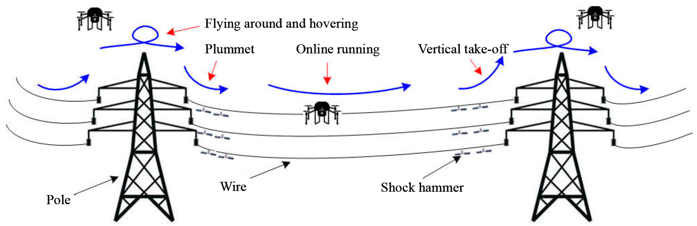
:1. Introduction
2. Inspection Drone Dynamic Model
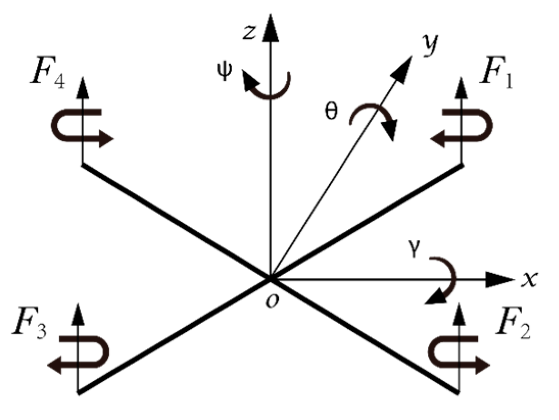
2.1. Establishment of Coordinate System
2.2. Establishment of Coordinate System
- The four-rotor aircraft is regarded as a rigid body, and its body structure is completely uniform and symmetrical.
- The origin O of the airframe coordinate system coincides with the origin O of the inertial coordinate system to ensure that the inertial matrix is a diagonal matrix in the rigid body coordinate system [20].
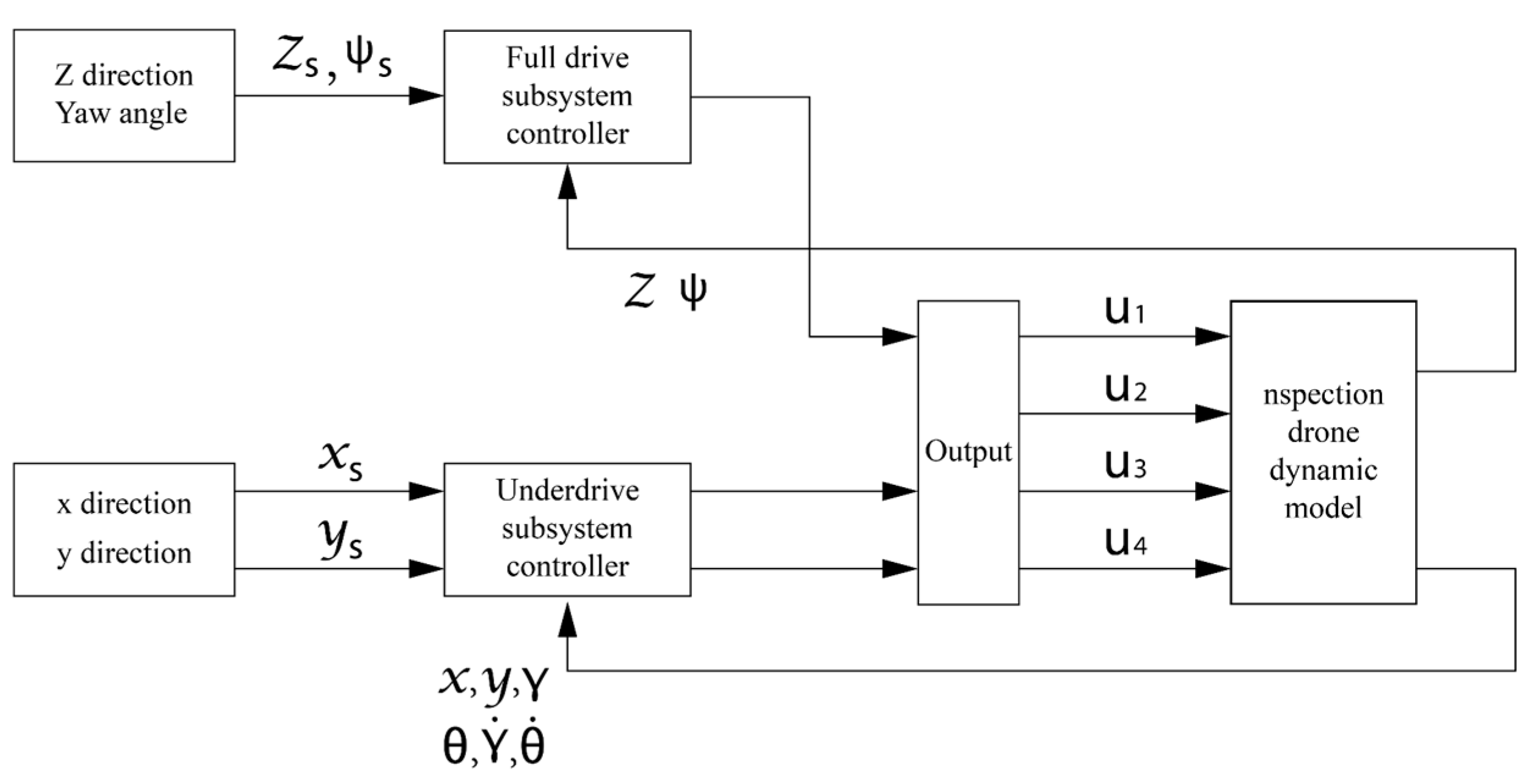
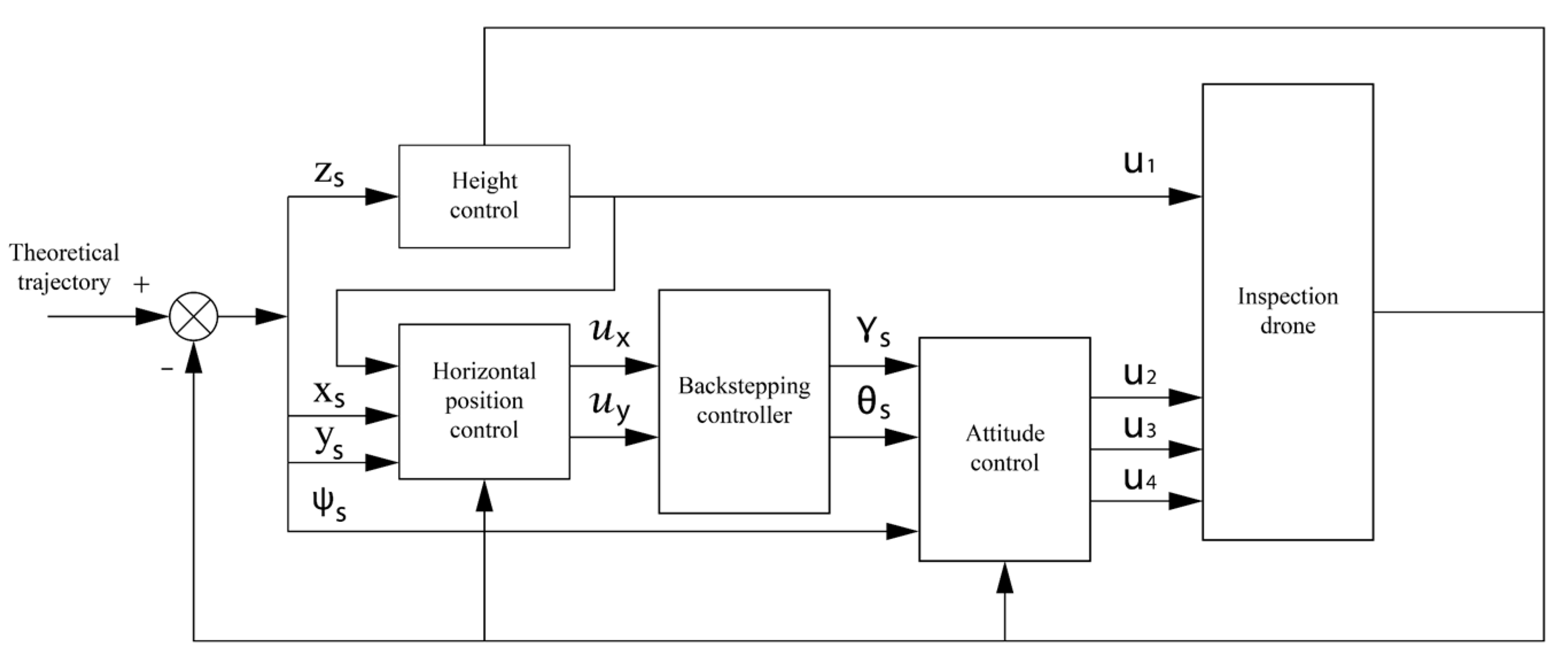
3. Control System Design
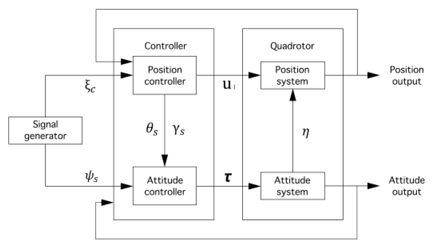
3.1. Controller Design Structure
3.2. Position Controller Design
3.3. Design of Attitude Tracking Controller
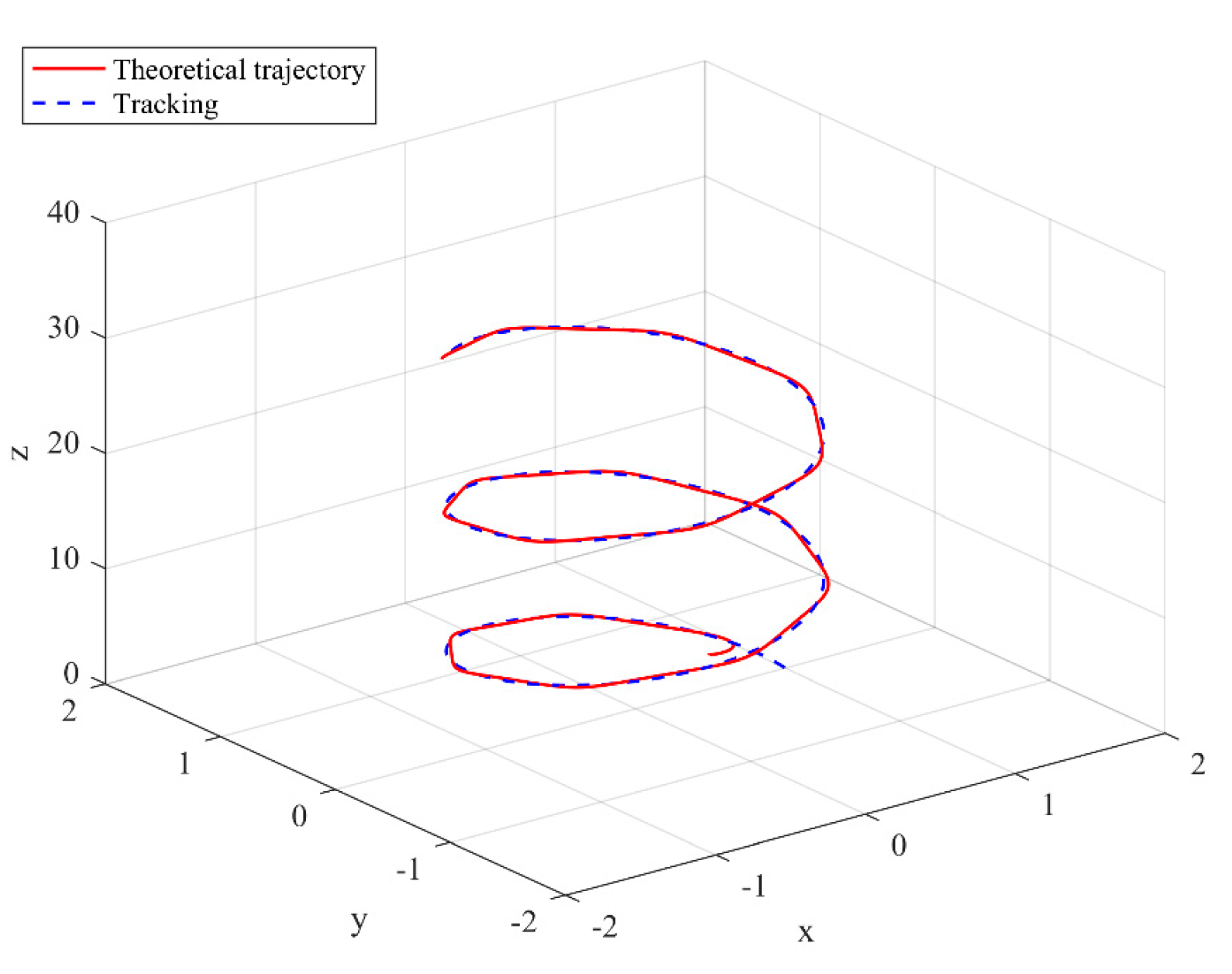
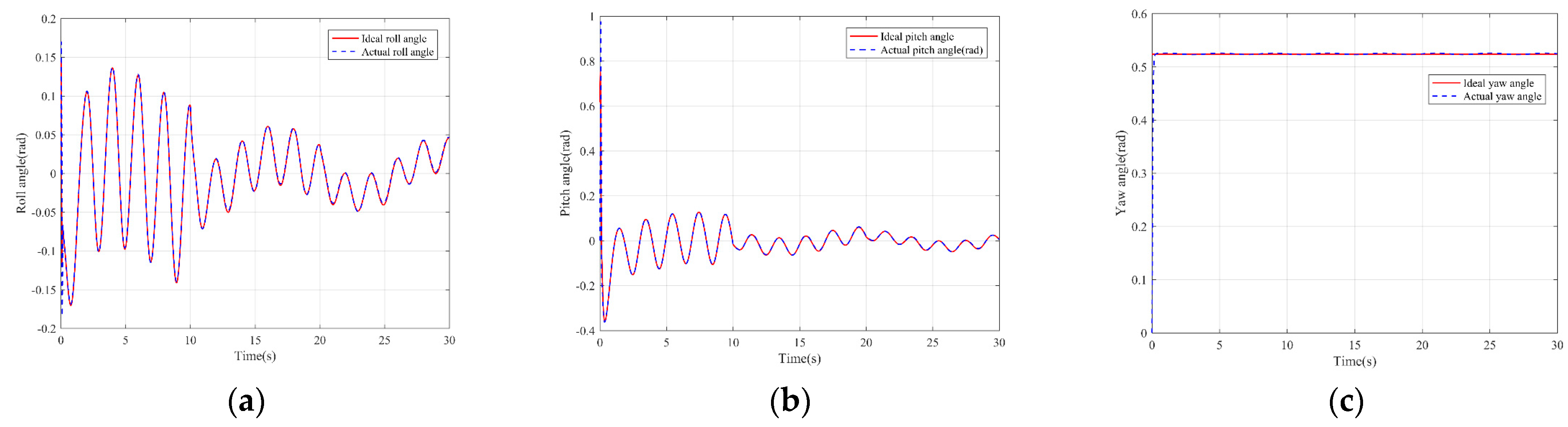
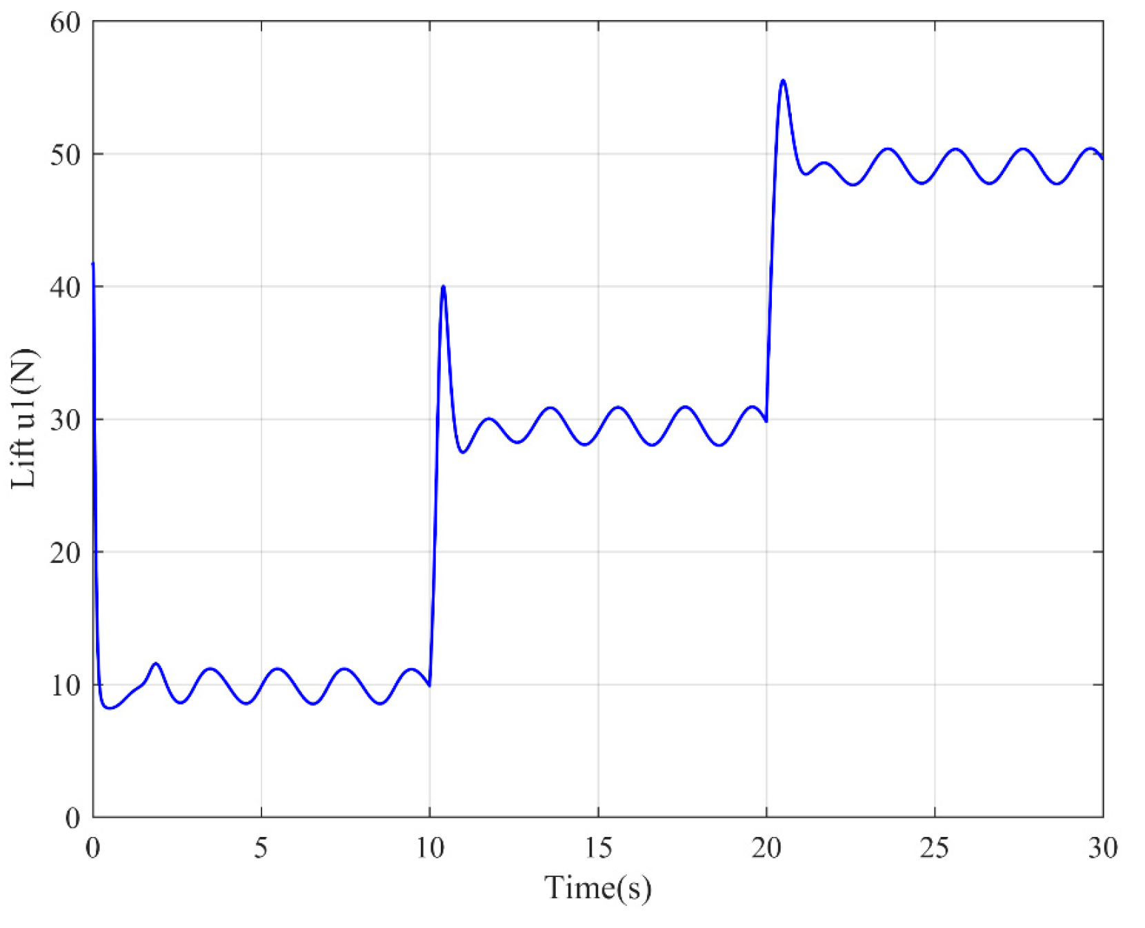
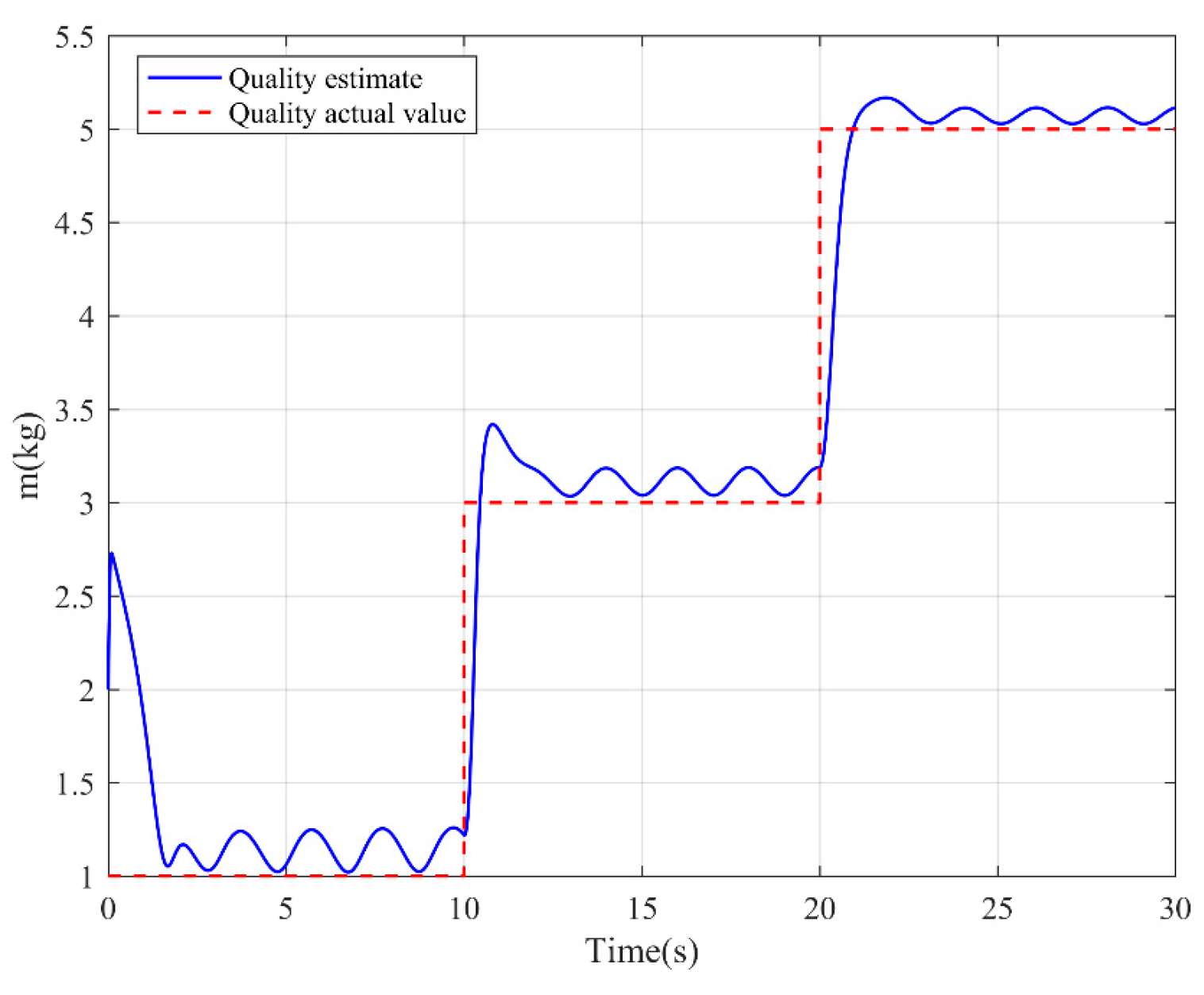
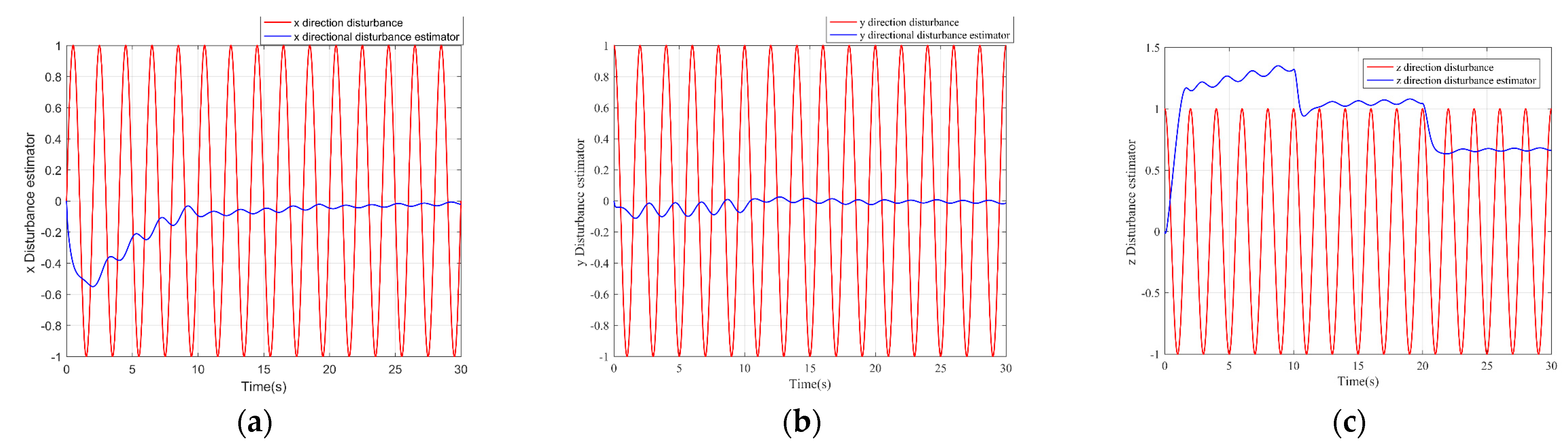
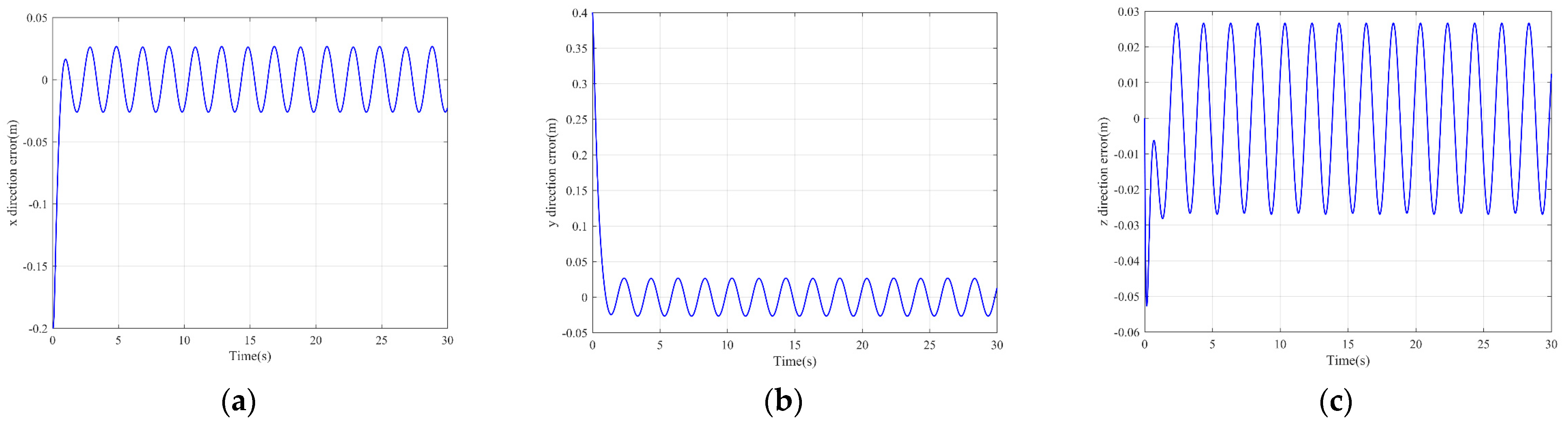
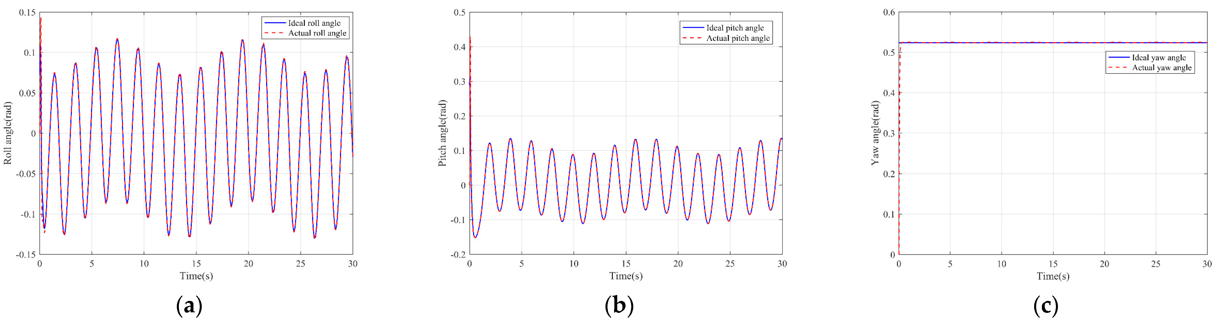
4. Simulation Research
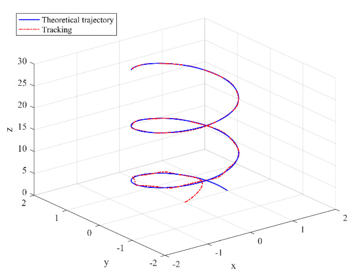
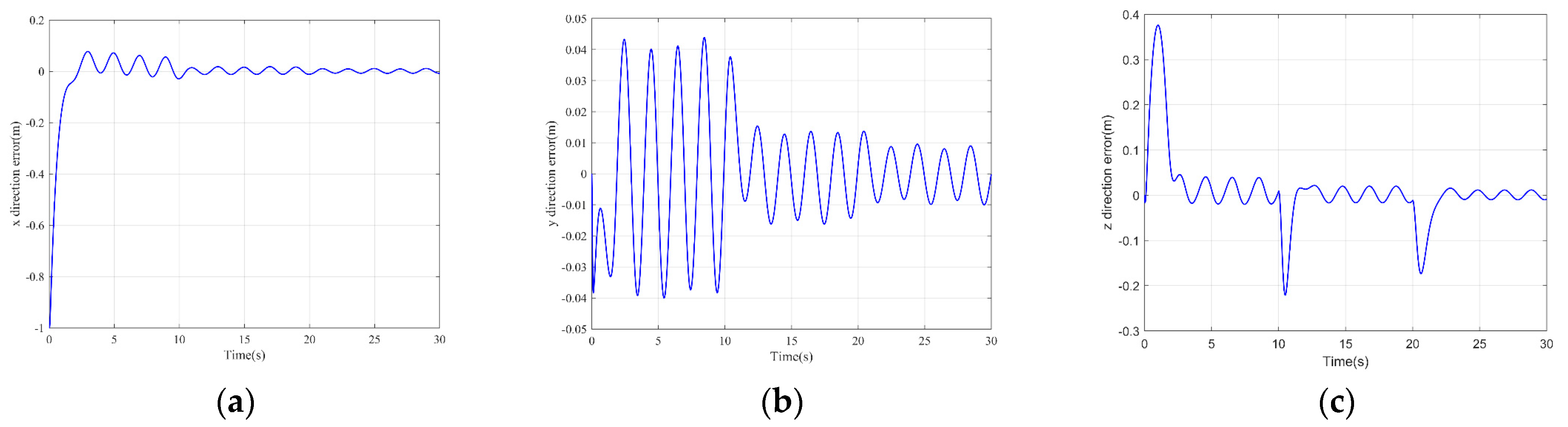
Simulation
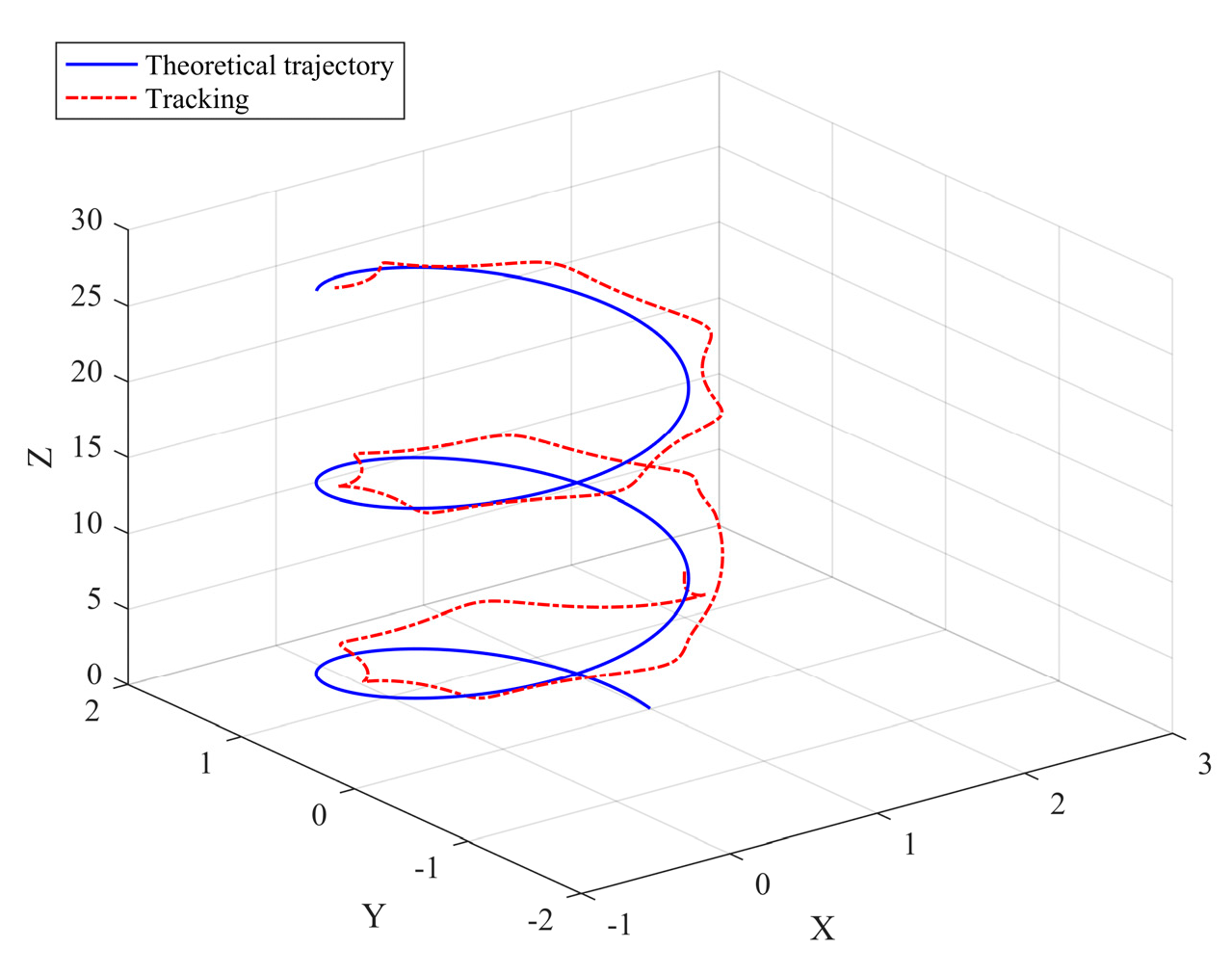
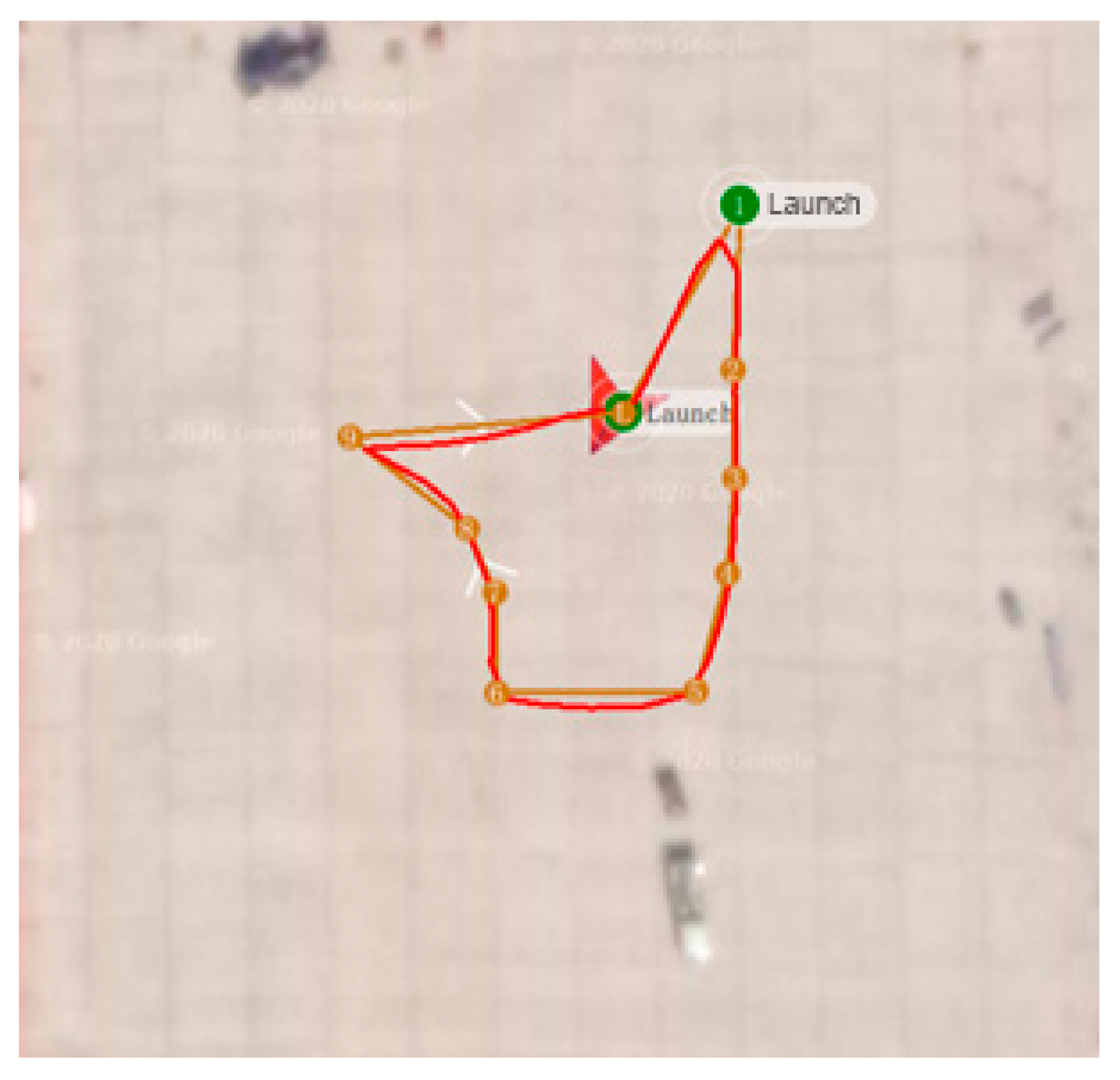
5. Experimental Design
5.1. Sliding Mode PID Control Group Experiment
5.2. Backstepping Control Group Experiment
6. Experimental Study
7. Discussion
- The inspection drone is an underdriven system where the control volume is less than the output volume.
- Jitter vibration will be generated near the transition to the slide surface during the control process.
- The actual altitude always has a constant small deviation from the ideal altitude after the trajectory tracking process is stabilized.
- The inner loop of attitude control and the outer loop of position control cannot be coordinated immediately during the continuous steering process.
8. Conclusions
Author Contributions
Funding
Funding
Institutional Review Board Statement
Informed Consent Statement
Conflicts of Interest
References
- Lopez Lopez, R.; Batista Sanchez, M.J.; Perez Jimenez, M.; Arrue, B.C.; Ollero, A. Autonomous UAV System for Cleaning Insulators in Power Line Inspection and Maintenance. Sensors 2021, 21, 8488. [Google Scholar] [CrossRef] [PubMed]
- Chang, C.-W.; Lo, L.-Y.; Cheung, H.C.; Feng, Y.; Yang, A.-S.; Wen, C.-Y.; Zhou, W. Proactive Guidance for Accurate UAV Landing on a Dynamic Platform: A Visual–Inertial Approach. Sensors 2022, 22, 404. [Google Scholar] [CrossRef] [PubMed]
- Tayyab, M.; Yuanqing, X.; Di-Hua, Z.; Dailiang, M. Trajectory tracking control of a VTOL unmanned aerial vehicle using offset-free tracking MPC. Chin. J. Aeronaut. 2020, 33, 2024–2042. [Google Scholar]
- Ma, H.; Xiong, Z.; Li, Y.; Liu, Z. Sliding Mode Control for Uncertain Discrete-Time Systems Using an Adaptive Reaching Law. IEEE Trans. Circuits Syst. II-Express Briefs 2022, 68, 722–726. [Google Scholar] [CrossRef]
- Xu, C.; Yin, C.; Han, W.; Wang, D. Two-UAV trajectory planning for cooperative target locating based on airborne visual tracking platform. Electron. Lett. 2020, 56, 301–303. [Google Scholar] [CrossRef]
- Jia, R.; Zong, X. Quadrotor UAV Trajectory Tracking Control based on ASMC and Improved ARDC. In Proceedings of the 2020 Chinese Automation Congress (CAC), Shanghai, China, 6–8 November 2020; pp. 6078–6083. [Google Scholar] [CrossRef]
- Xu, J.; Cai, C.; Li, Y.; Xu, J. Double closed-loop trajectory tracking and control of a small quadrotor UAV. Control. Theory Appl. 2015, 32, 1335–1342. [Google Scholar]
- Wang, S.; Yin, X.; Li, P.; Zhang, M.; Wang, X. Trajectory Tracking Control for Mobile Robots Using Reinforcement Learning and PID. Iran. J. Sci. Technol. Trans. Electr. Eng. 2020, 44, 1059–1068. [Google Scholar] [CrossRef]
- Yao, Q. Adaptive finite-time sliding mode control design for finite-time fault-tolerant trajectory tracking of marine vehicles with input saturation. J. Frankl. Inst. 2020, 357, 13593–13619. [Google Scholar] [CrossRef]
- Gu, J.; Sun, R.; Chen, J. Improved Back-Stepping Control for Nonlinear Small UAV Systems with Transient Prescribed Performance Design. IEEE Access 2021, 9, 128786–128798. [Google Scholar] [CrossRef]
- Li, J.; Liu, J.; Sun, Z. Quadrotor Trajectory Tracking Control Based on Backstepping Method. J. Qufu Norm. Univ. 2020, 46, 47–50. [Google Scholar]
- Shen, Z.; Cao, X. Output feedback control of input constrained quadrotor aircraft trajectory tracking dynamic surface based on extended observer. Syst. Eng. Electron. Technol. 2018, 40, 2766–2774. [Google Scholar]
- Chen, X. Hybrid trajectory tracking control algorithm for quadrotor aircraft. Electro-Opt. Control. 2020, 27, 58–62,67. [Google Scholar]
- Wang, N.; Wang, Y. Adaptive dynamic surface trajectory tracking control of quadrotor aircraft based on Fuzzy Uncertain observer. J. Autom. 2018, 44, 685–695. [Google Scholar]
- Luna, M.A.; Ale Isaac, M.S.; Ragab, A.R.; Campoy, P.; Flores Peña, P.; Molina, M. Fast Multi-UAV Path Planning for Optimal Area Coverage in Aerial Sensing Applications. Sensors 2022, 22, 2297. [Google Scholar] [CrossRef] [PubMed]
- López, B.; Muñoz, J.; Quevedo, F.; Monje, C.A.; Garrido, S.; Moreno, L.E. Path Planning and Collision Risk Management Strategy for Multi-UAV Systems in 3D Environments. Sensors 2021, 21, 4414. [Google Scholar] [CrossRef]
- Mehmood, Y.; Aslam, J.; Ullah, N.; Chowdhury, M.S.; Techato, K.; Alzaed, A.N. Adaptive Robust Trajectory Tracking Control of Multiple Quad-Rotor UAVs with Parametric Uncertainties and Disturbances. Sensors 2021, 21, 2401. [Google Scholar] [CrossRef]
- Tang, Y.R.; Xiao, X.; Li, Y. Nonlinear dynamic modeling and hybrid control design with dynamic compensator for a small-scale UAV quadrotor. Measurement 2017, 109, 51–64. [Google Scholar] [CrossRef]
- Yuan, D.; Wang, Y. Data Driven Model-Free Adaptive Control Method for Quadrotor Formation Trajectory Tracking Based on RISE and ISMC Algorithm. Sensors 2021, 21, 1289. [Google Scholar] [CrossRef]
- An, S.; Liu, X.; Hou, K.; Xu, X. Establishment of the dynamic model of the electric power system of a slight UAV. J. Harbin Univ. Sci. Technol. 2020, 25, 33–39. [Google Scholar]
- Qian, L.; Li, Z.; Wang, Y. Research on optimization design of quadrotor control system. Comput. Simul. 2018, 35, 18–23. [Google Scholar]
- Yu, S. Research on Intelligent Control Method of Quadrotor Aircraft; China University of Petroleum (East China): Beijing, China, 2018. [Google Scholar]
- Farrell, J.; Sharma, M.; Polycarpou, M. Backstepping-Based Flight Control with Adaptive Function Approximation. J. Guid. Control. Dyn. 2005, 28, 1089–1102. [Google Scholar] [CrossRef]
- Wang, L.; Wang, M. Analysis of the construction of Lyapunov functions for a class of third order nonlinear systems. J. Appl. Math. 1983, 6, 309–323. [Google Scholar]
- Iason, K.; Ioannis, M.; Nikos, N.; Pitas, I. Shot type constraints in UAV cinematography for autonomous target tracking. Inf. Sci. 2020, 506, 273–294. [Google Scholar]
- Marino, R.; Respondek, W.; Van der Schaft, A.J. Almost Disturbance Decoupling for Single-Input Single-Output Nonlinear Systems. Trans. Autom. Control. IEEE 1989, 34, 1013–1017. [Google Scholar] [CrossRef] [Green Version]


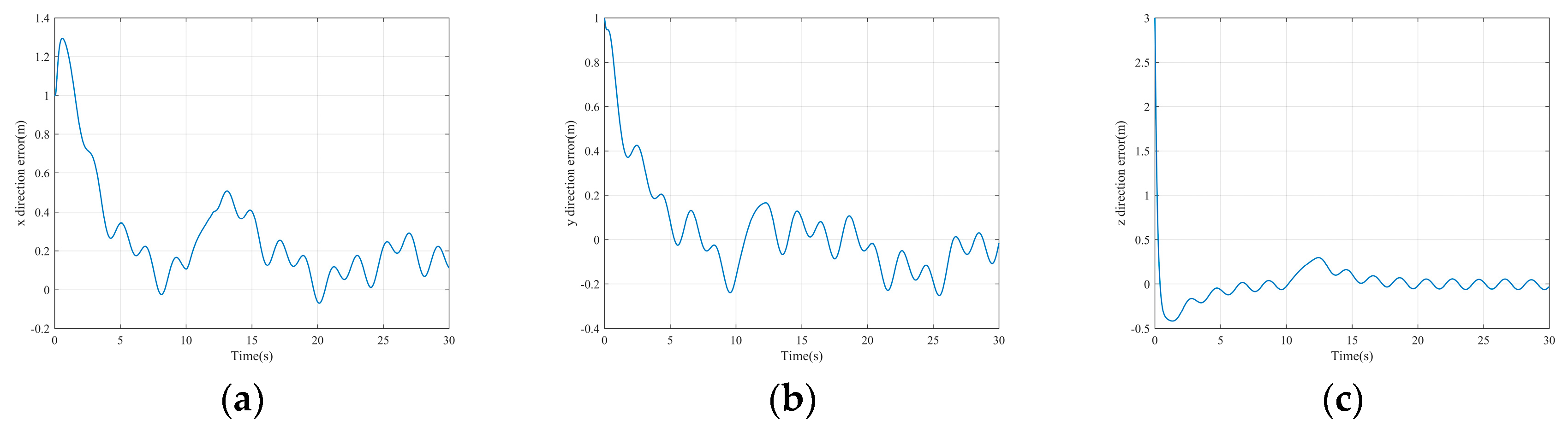
| Control Method | x-Direction Tracking Error Range | y-Direction Tracking Error Range | z-Direction Tracking Error Range |
|---|---|---|---|
| Sliding Mode Adaptive Robustness | −0.21–0.16 | −0.31–0.58 | −0.63–1.21 |
| Sliding Mode PID | −0.23–0.36 | −0.86–0.79 | −0.59–1.32 |
| backstepping control | −0.56–1.21 | −1.52–1.63 | −1.63–1.82 |
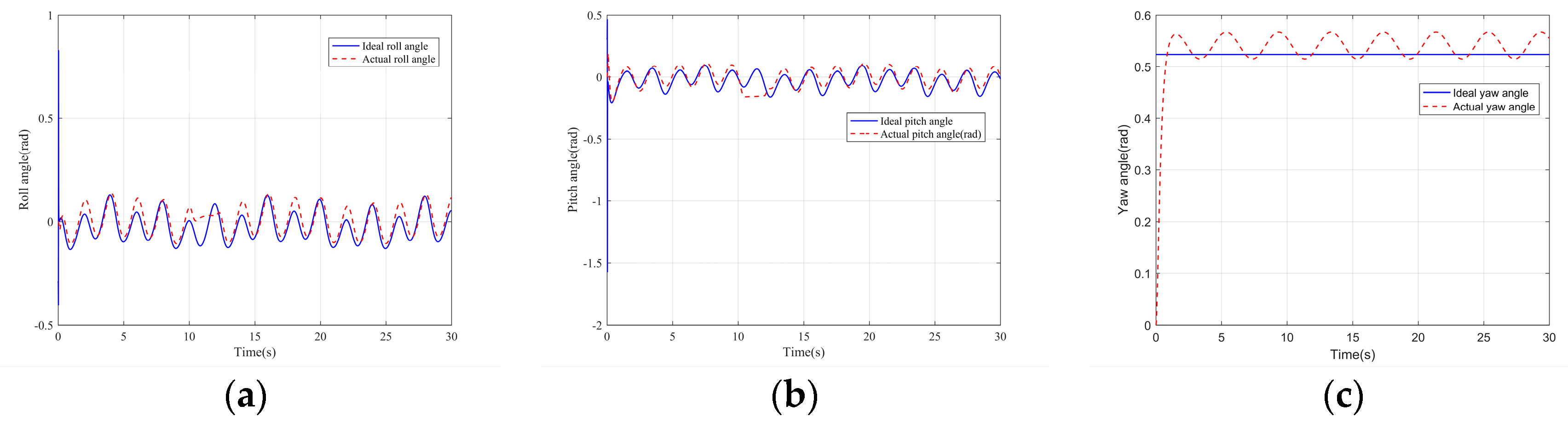
| Control Method | Roll Angle | Pitch Angle | Yaw Angle |
|---|---|---|---|
| Sliding Mode Adaptive Robustness | −0.5–0.75 | −0.04–0.58 | −0.21–0.36 |
| Sliding Mode PID | −0.86–0.95 | −0.5–0.36 | −0.31–0.48 |
| backstepping control | −0.98–1.025 | −0.93–0.86 | −1.26–1.10 |
Publisher’s Note: MDPI stays neutral with regard to jurisdictional claims in published maps and institutional affiliations. |
© 2022 by the authors. Licensee MDPI, Basel, Switzerland. This article is an open access article distributed under the terms and conditions of the Creative Commons Attribution (CC BY) license (https://creativecommons.org/licenses/by/4.0/).
Share and Cite
Yang, M.; Zhou, Z.; You, X. Research on Trajectory Tracking Control of Inspection UAV Based on Real-Time Sensor Data. Sensors 2022, 22, 3648. https://doi.org/10.3390/s22103648
Yang M, Zhou Z, You X. Research on Trajectory Tracking Control of Inspection UAV Based on Real-Time Sensor Data. Sensors. 2022; 22(10):3648. https://doi.org/10.3390/s22103648
Chicago/Turabian StyleYang, Mingbo, Ziyang Zhou, and Xiangming You. 2022. "Research on Trajectory Tracking Control of Inspection UAV Based on Real-Time Sensor Data" Sensors 22, no. 10: 3648. https://doi.org/10.3390/s22103648
APA StyleYang, M., Zhou, Z., & You, X. (2022). Research on Trajectory Tracking Control of Inspection UAV Based on Real-Time Sensor Data. Sensors, 22(10), 3648. https://doi.org/10.3390/s22103648