
Multisensor Data Fusion for Localization of Pollution Sources in Wastewater Networks


Abstract
:1. Introduction
Related Work
- The pollutant does not react with other substances.
- The pollutant gradually dilutes with the water flow.
- The running speed of the pollutant is consistent with the flow velocity of the pipe segment.
- Pollutants are injected into the network only through the nodes.
- The probability of injection for all nodes is equal.
- The sensors can monitor water properties in real-time.
2. Methods
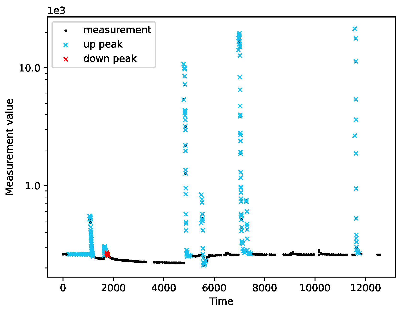
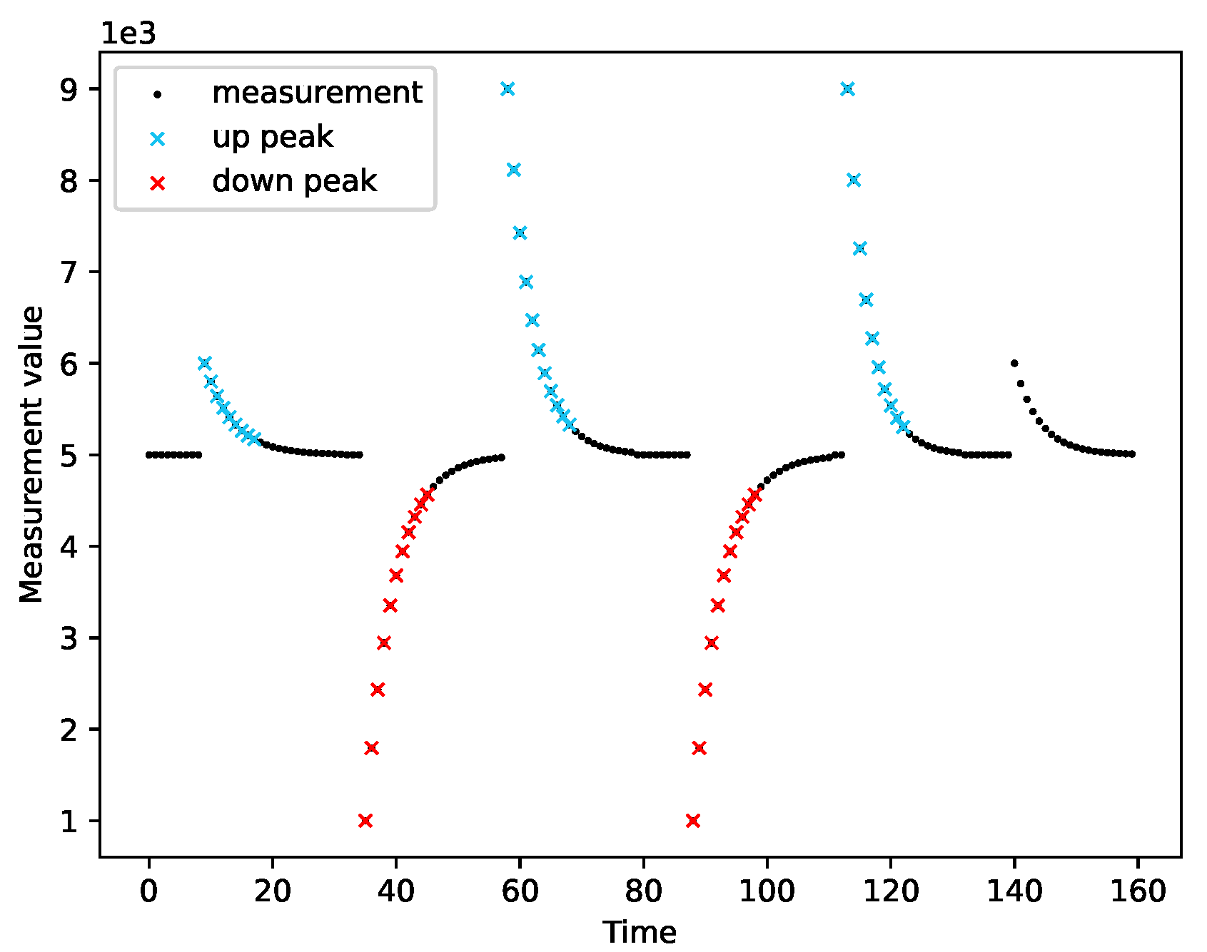
2.1. Adaptive Peak Detection
| Algorithm 1: Peak detection. |
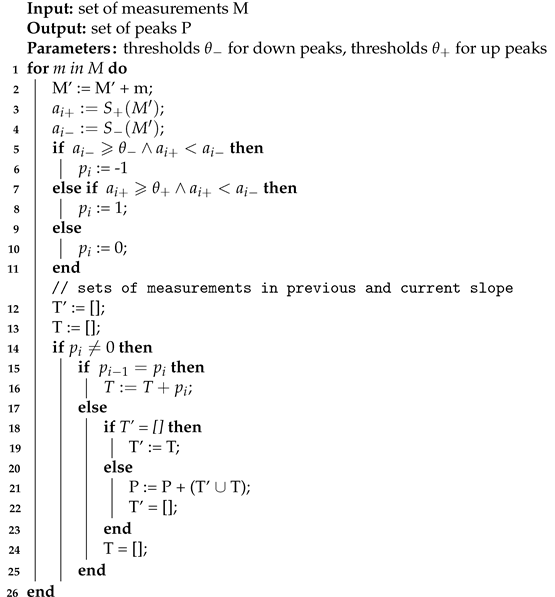 |
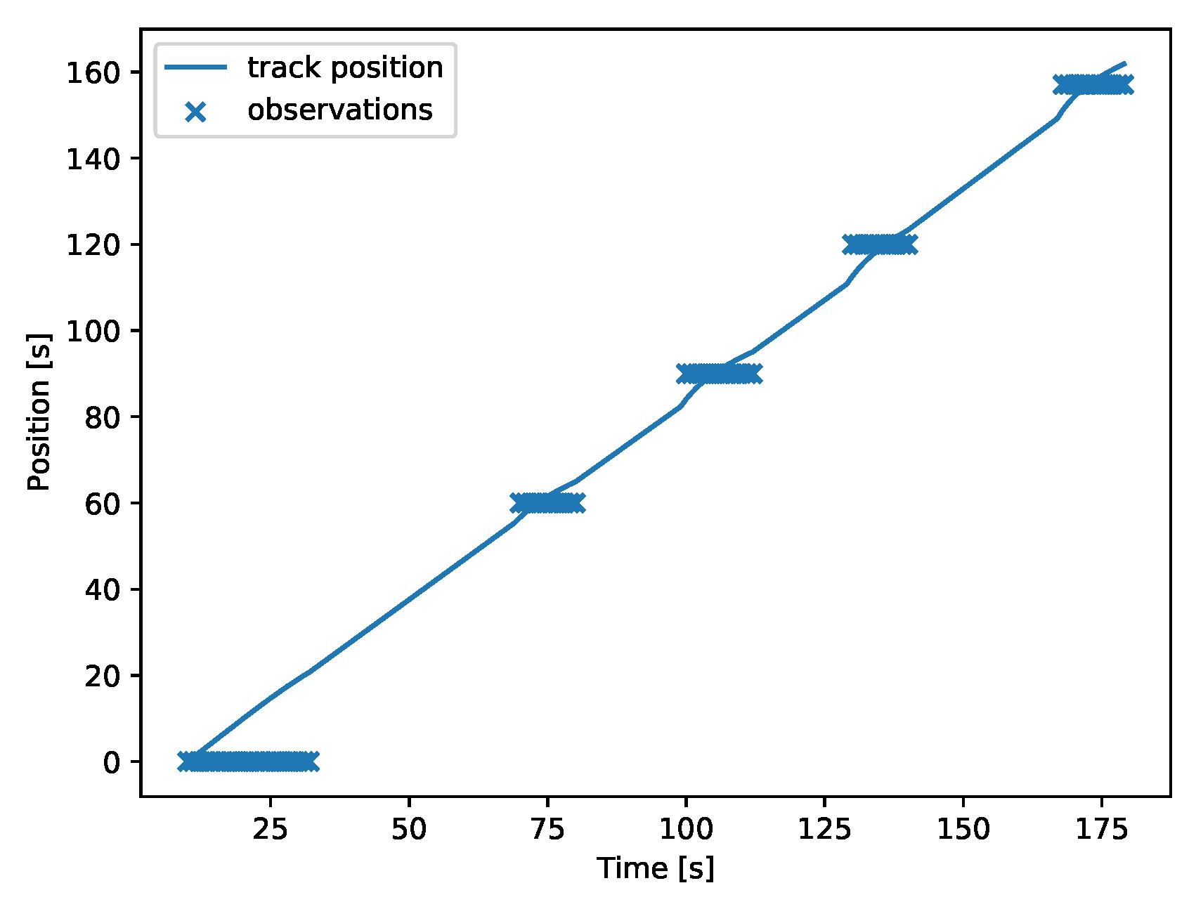
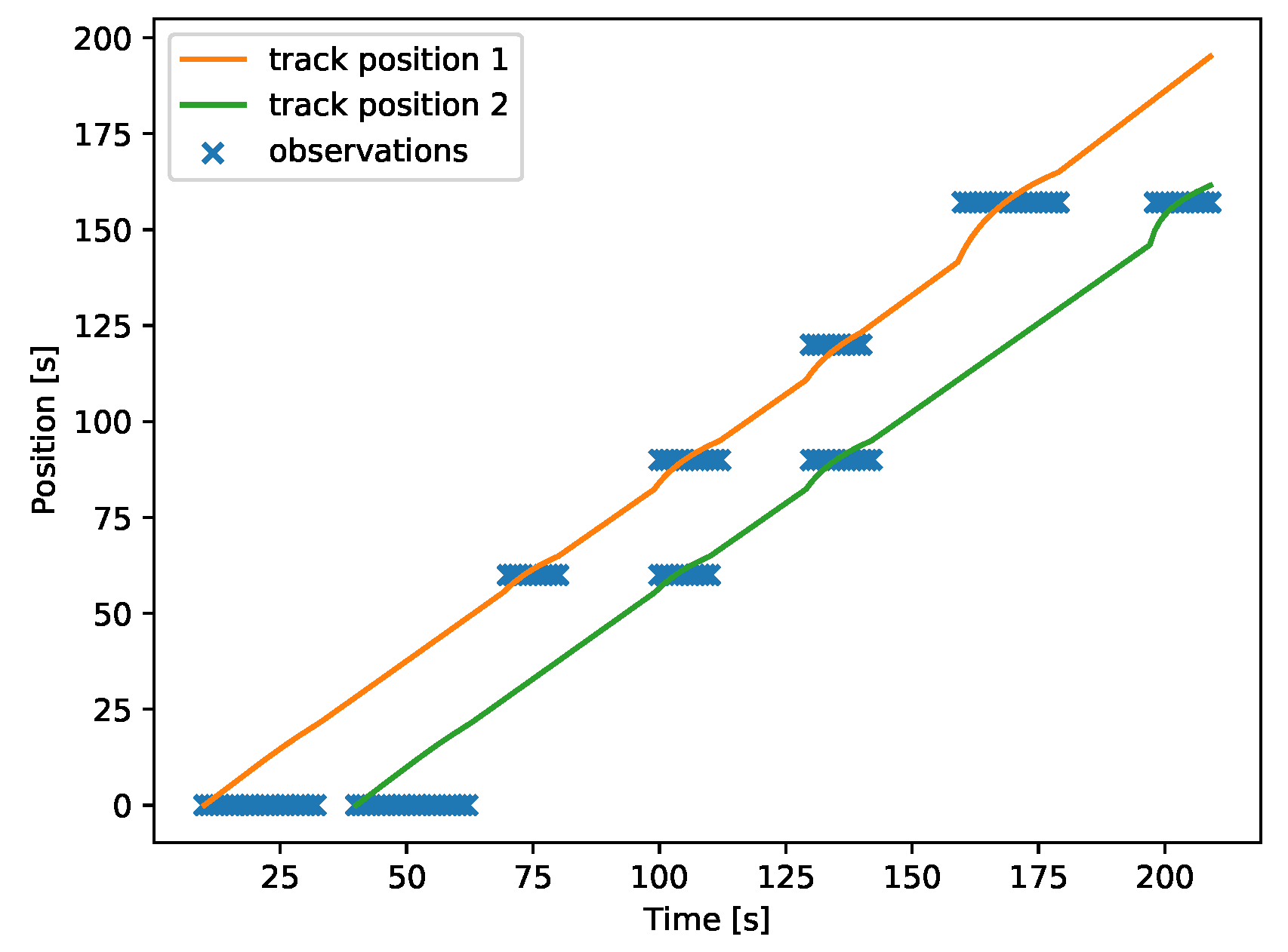
2.2. Tracking in DAGs
2.3. Better Amount Approximation with Flow Rate
3. Results
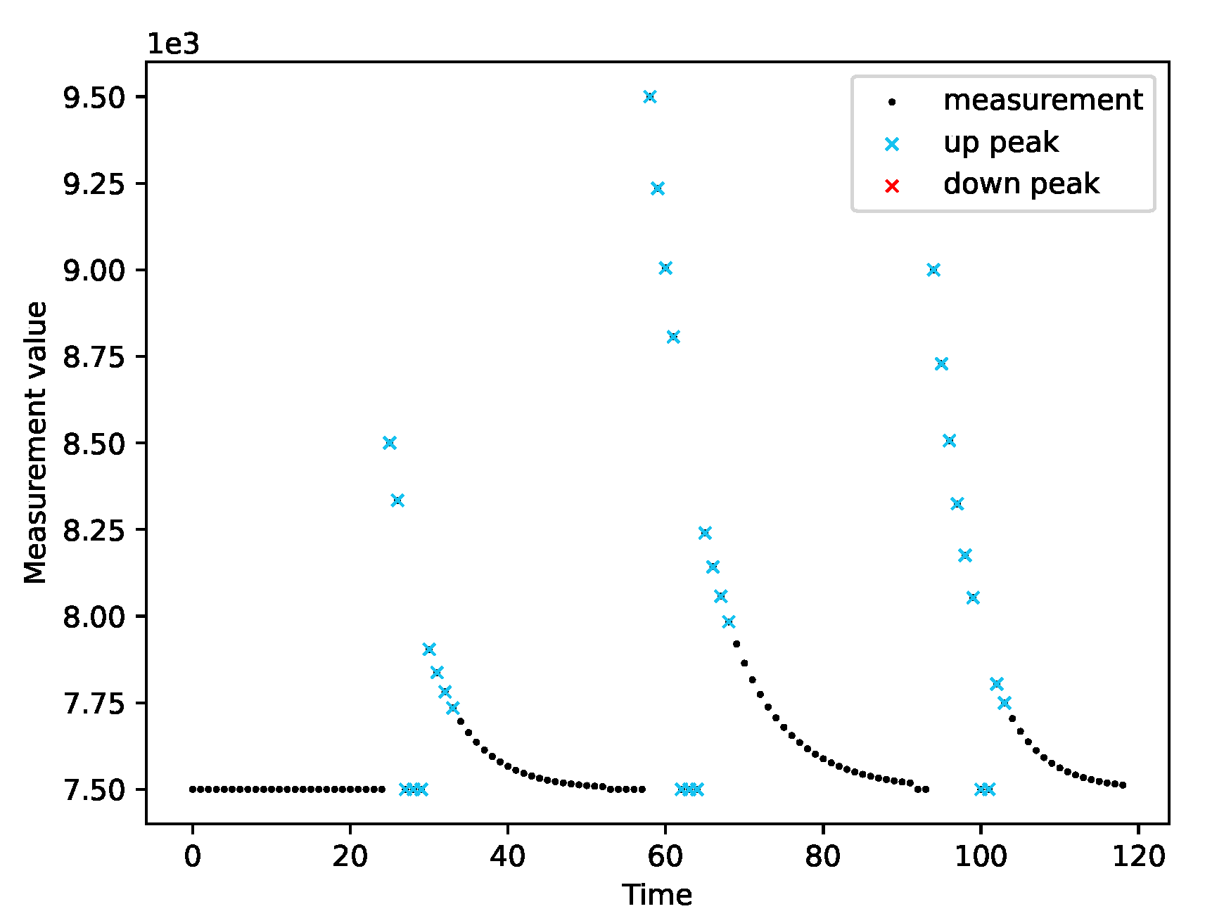
3.1. Exponential Signal Generator
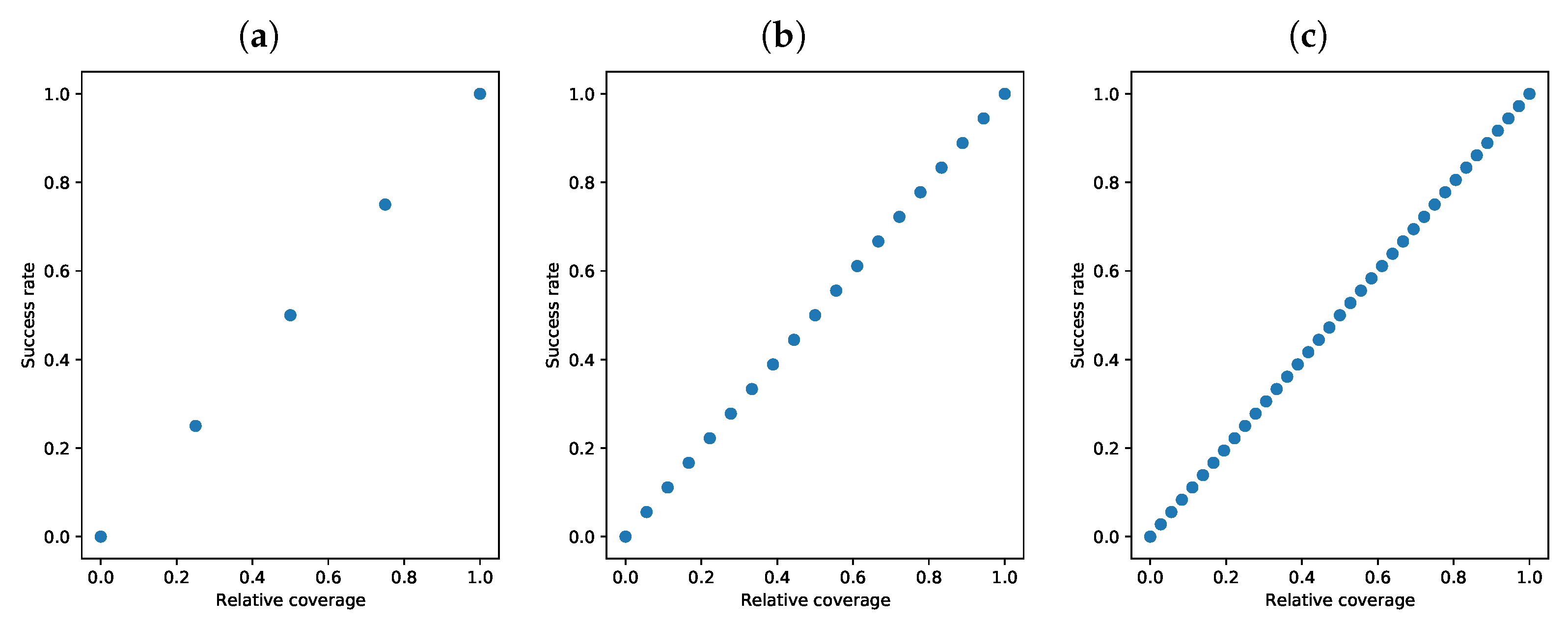
3.2. Success Rate
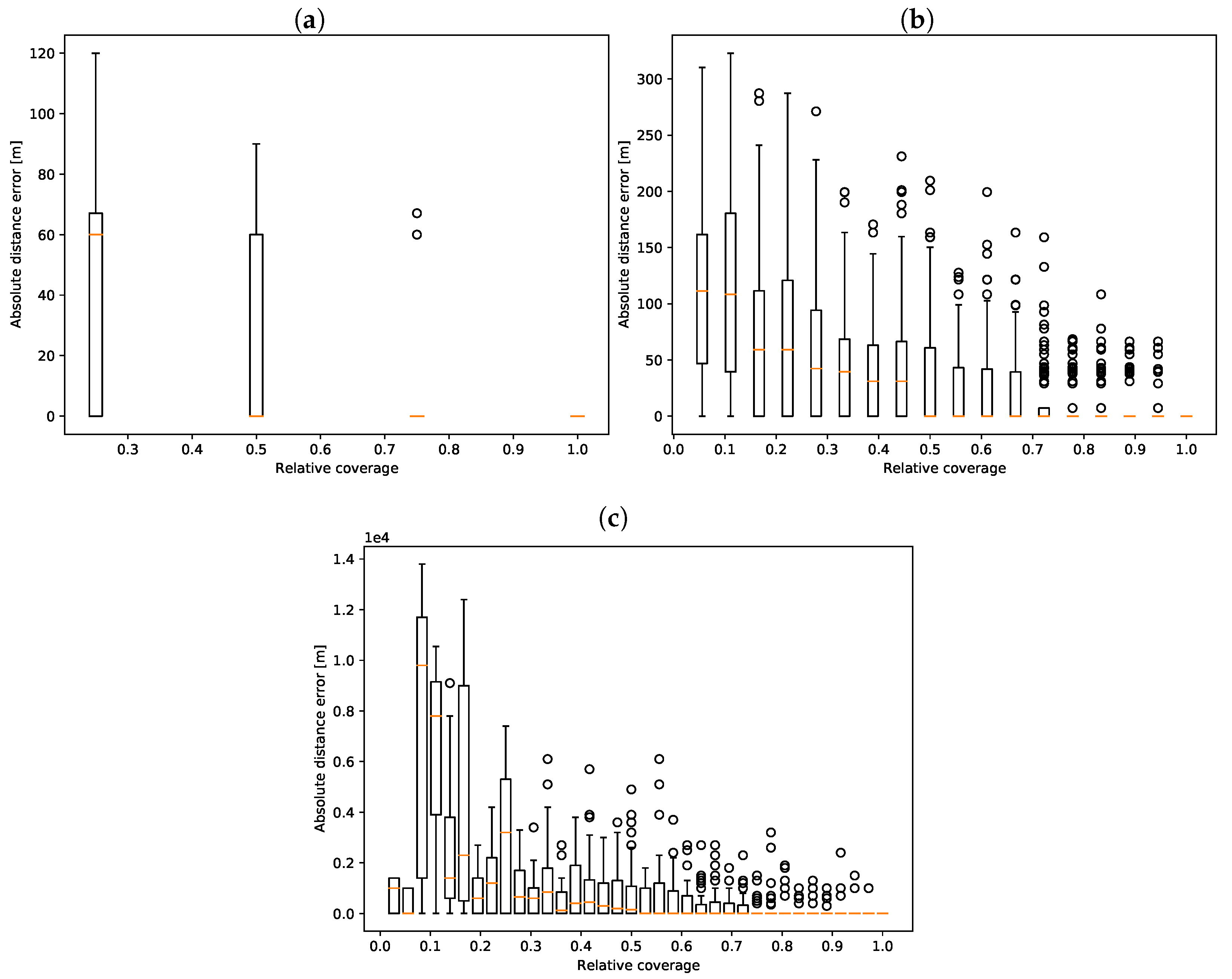
3.3. Distance Error
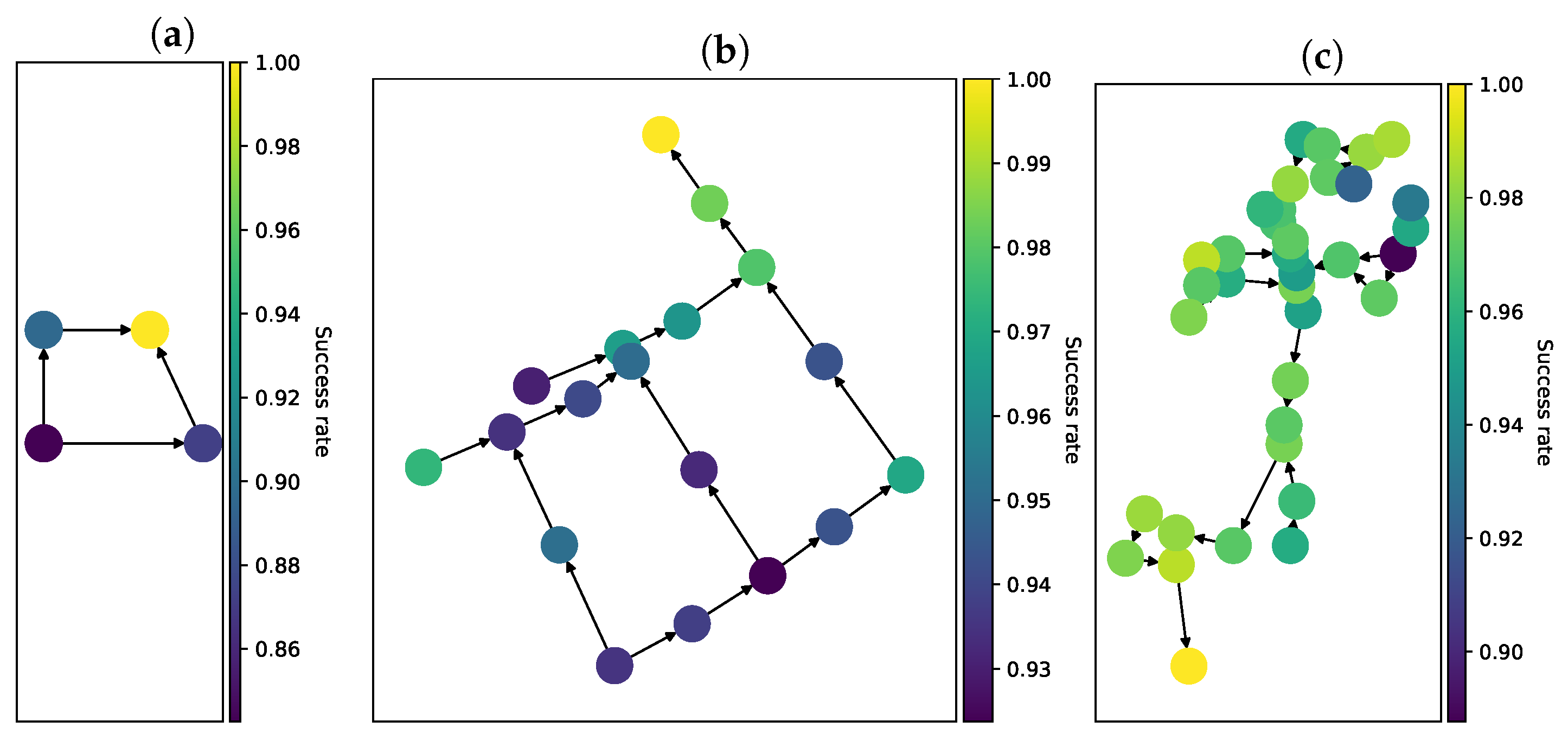
3.4. Sensor Success Rate
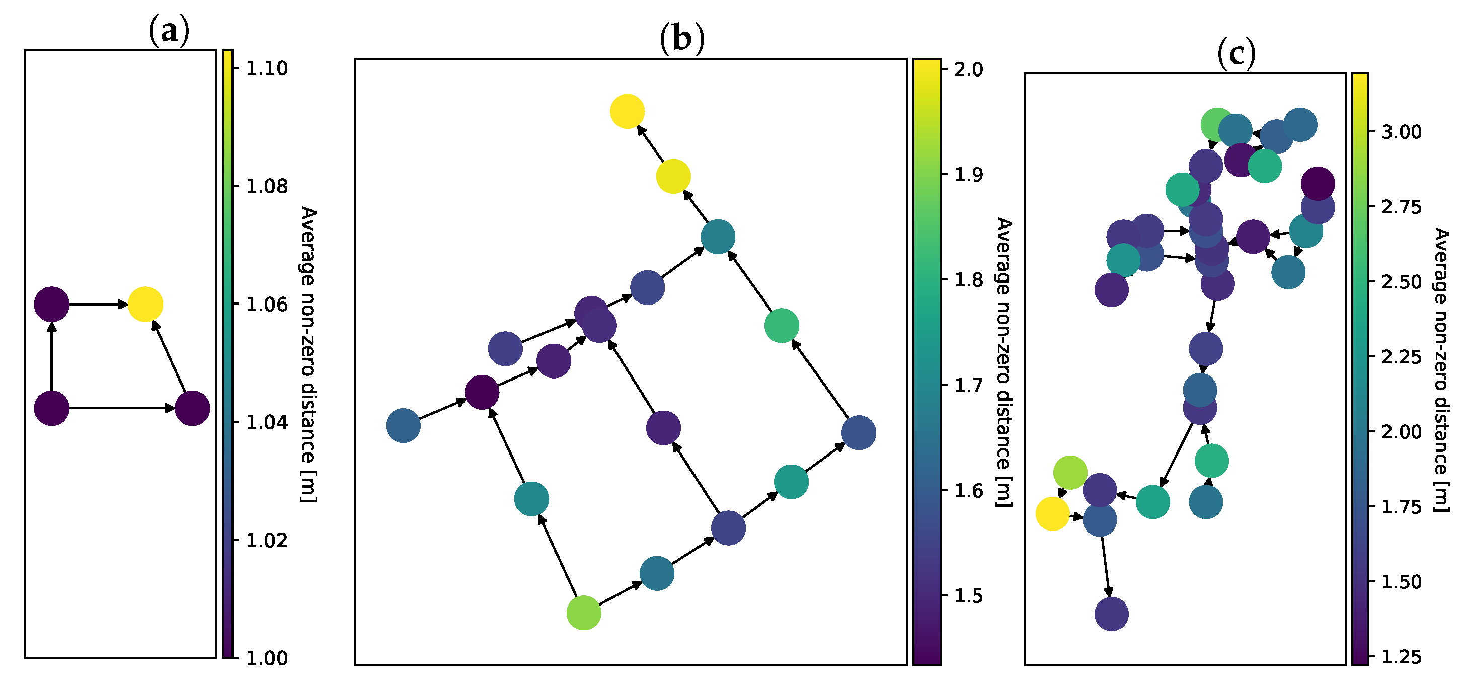
3.5. Sensor Distance Error
3.6. Peak Detection
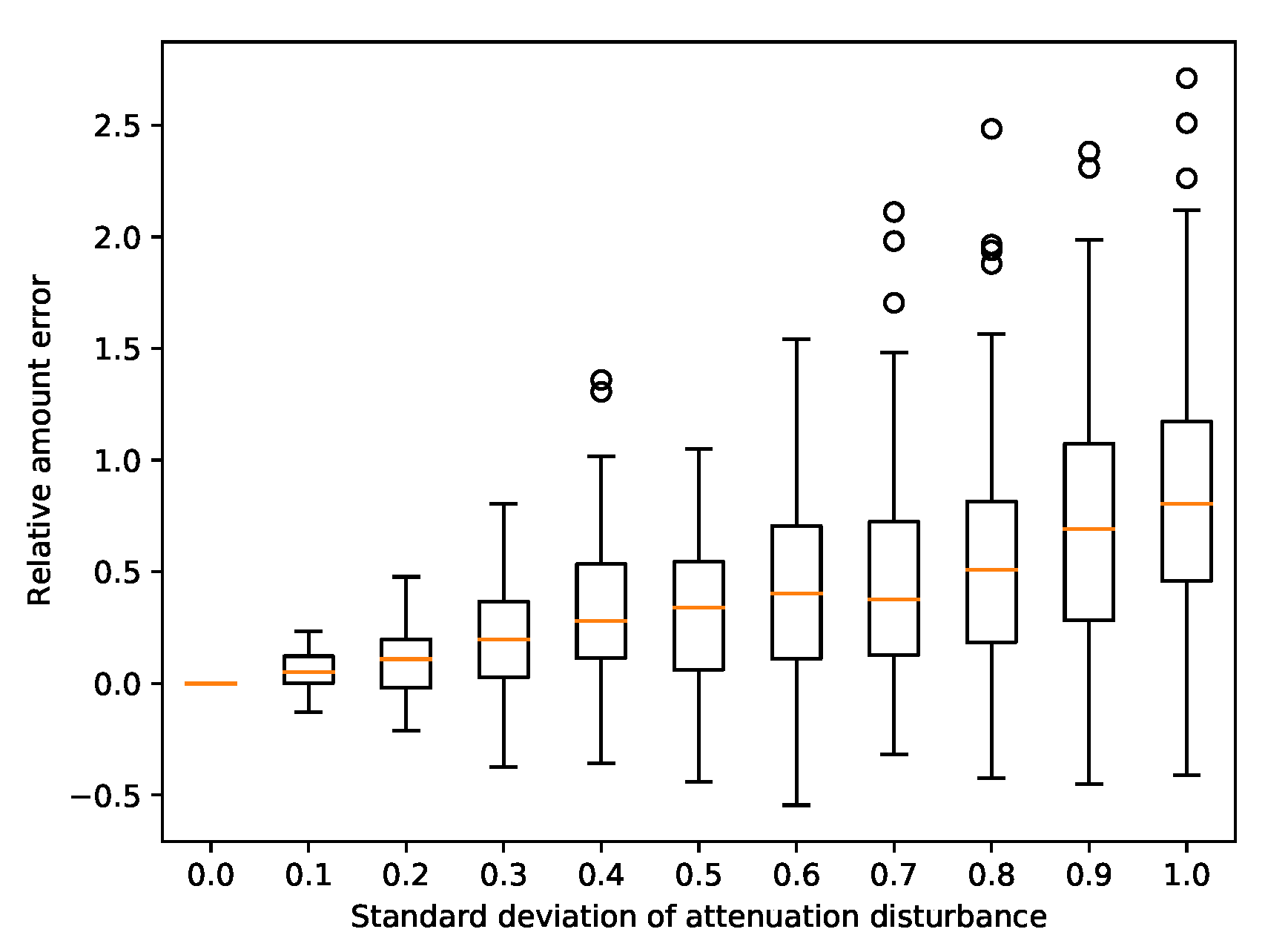
3.7. Attenuation in Quantification
3.8. Multipath Tracking
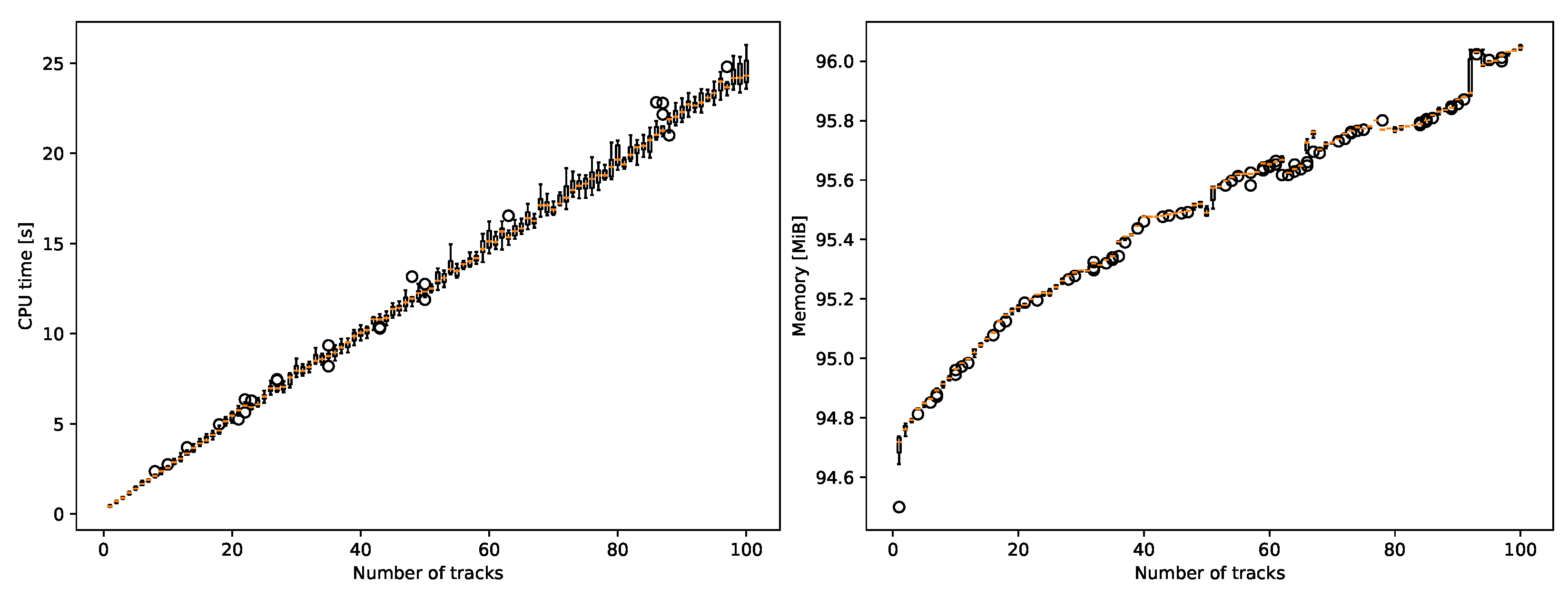
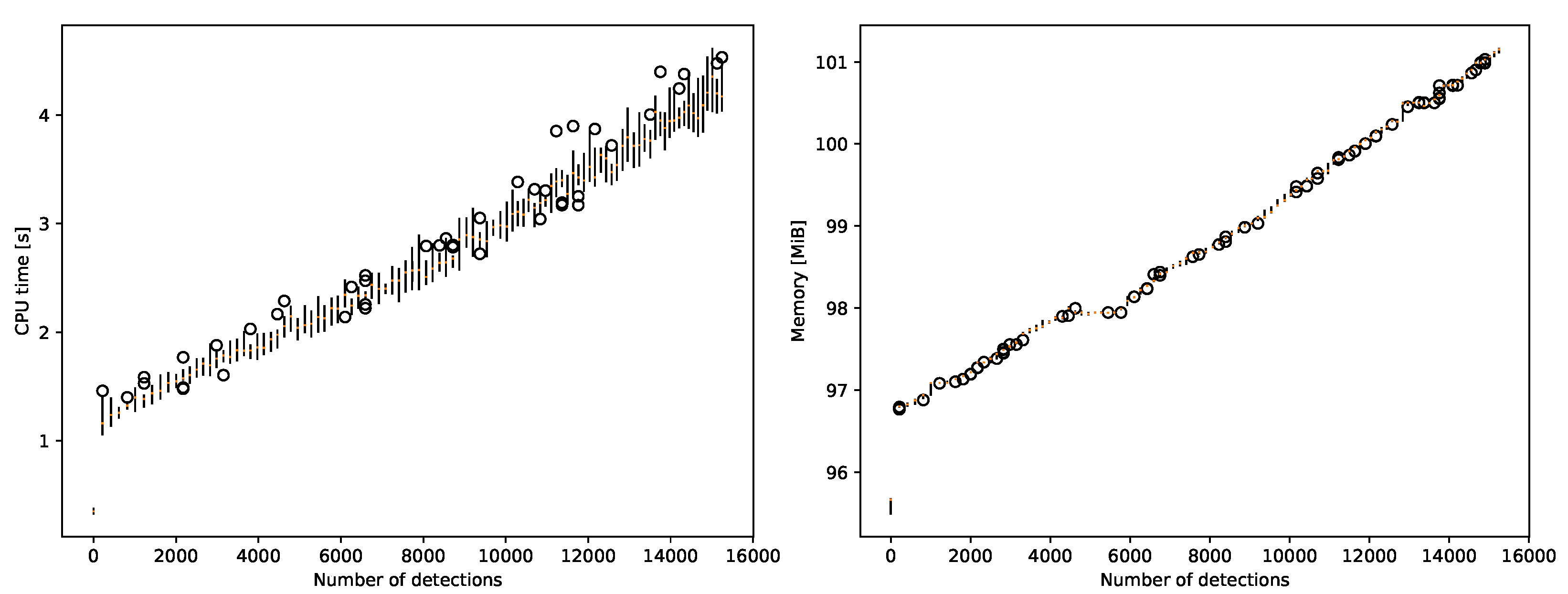
3.9. Resource Usage
4. Discussion
5. Conclusions
Author Contributions
Funding
Institutional Review Board Statement
Informed Consent Statement
Data Availability Statement
Acknowledgments
Conflicts of Interest
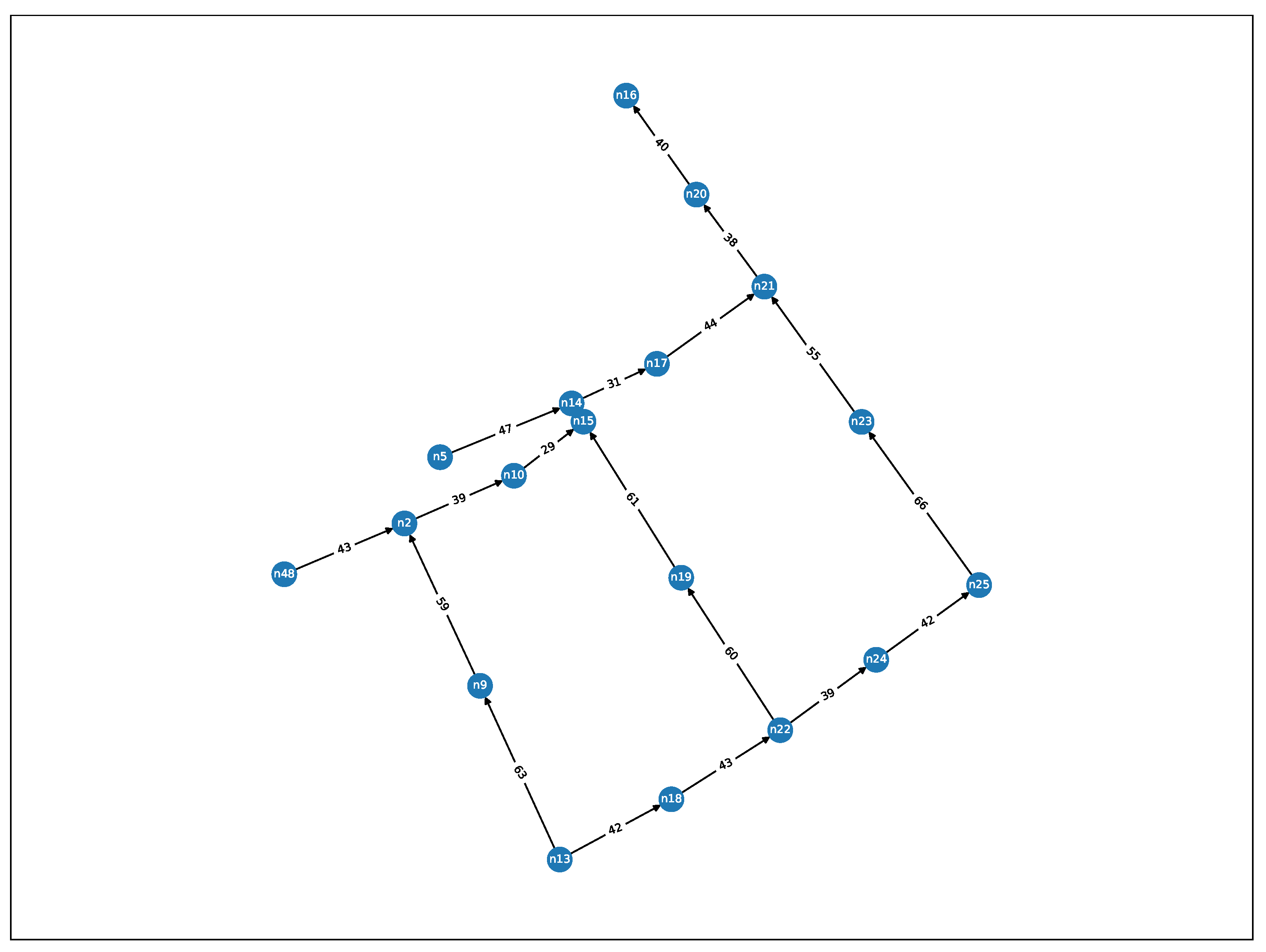
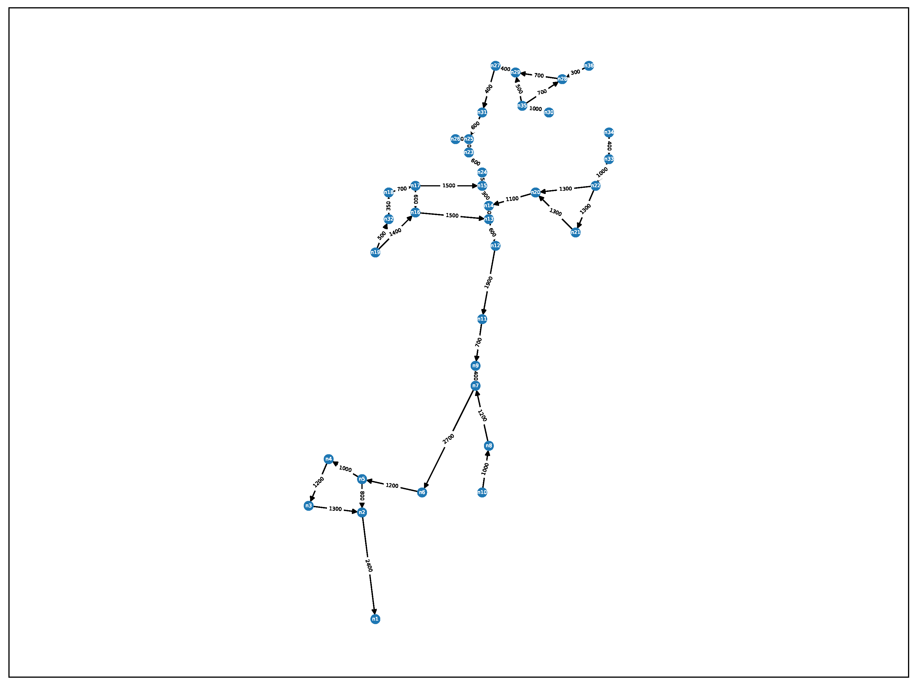
Appendix A. Detailed Renders of Networks Used in Experiments

References
- Micromole. Micromole—Sewage Monitoring System for Tracking Synthetic Drug Laboratories. Available online: http://www.micromole.eu (accessed on 17 October 2019).
- SYSTEM. H2020 SYSTEM—SYnergy of Integrated Sensors and Technologies for Urban Secured Environment. Fact Sheet Available at EC Website. Under Project ID 787128. Available online: https://cordis.europa.eu/project/rcn/220304/factsheet/en (accessed on 12 October 2021).
- De Vito, S.; Fattoruso, G.; Esposito, E.; Salvato, M.; Agresta, A.; Panico, M.; Leopardi, A.; Formisano, F.; Buonanno, A.; Veneri, P.D.; et al. A distributed sensor network for waste water management plant protection. In Convegno Nazionale Sensori; Springer: Cham, Switzerland, 2016; pp. 303–314. [Google Scholar]
- Lepot, M.; Makris, K.F.; Clemens, F.H. Detection and quantification of lateral, illicit connections and infiltration in sewers with Infra-Red camera: Conclusions after a wide experimental plan. Water Res. 2017, 122, 678–691. [Google Scholar] [CrossRef]
- Tan, F.H.S.; Park, J.R.; Jung, K.; Lee, J.S.; Kang, D.K. Cascade of one class classifiers for water level anomaly detection. Electronics 2020, 9, 1012. [Google Scholar] [CrossRef]
- Tashman, Z.; Gorder, C.; Parthasarathy, S.; Nasr-Azadani, M.M.; Webre, R. Anomaly detection system for water networks in northern ethiopia using bayesian inference. Sustainability 2020, 12, 2897. [Google Scholar] [CrossRef] [Green Version]
- Zhang, D.; Heery, B.; O’Neil, M.; Little, S.; O’Connor, N.E.; Regan, F. A low-cost smart sensor network for catchment monitoring. Sensors 2019, 19, 2278. [Google Scholar] [CrossRef] [PubMed] [Green Version]
- Perfido, D.; Messervey, T.; Zanotti, C.; Raciti, M.; Costa, A. Automated leak detection system for the improvement of water network management. In Proceedings of the Multidisciplinary Digital Publishing Institute Proceedings, Online, 15–30 November 2016; Volume 1, p. 28. [Google Scholar]
- Rojek, I.; Studzinski, J. Detection and localization of water leaks in water nets supported by an ICT system with artificial intelligence methods as a way forward for smart cities. Sustainability 2019, 11, 518. [Google Scholar] [CrossRef] [Green Version]
- Ji, H.W.; Yoo, S.S.; Lee, B.J.; Koo, D.D.; Kang, J.H. Measurement of wastewater discharge in sewer pipes using image analysis. Water 2020, 12, 1771. [Google Scholar] [CrossRef]
- Kuchmenko, T.A.; Lvova, L.B. A perspective on recent advances in piezoelectric chemical sensors for environmental monitoring and foodstuffs analysis. Chemosensors 2019, 7, 39. [Google Scholar] [CrossRef] [Green Version]
- Pisa, I.; Santín, I.; Vicario, J.L.; Morell, A.; Vilanova, R. ANN-based soft sensor to predict effluent violations in wastewater treatment plants. Sensors 2019, 19, 1280. [Google Scholar] [CrossRef] [PubMed] [Green Version]
- Emke, E.; Vughs, D.; Kolkman, A.; de Voogt, P. Wastewater-based epidemiology generated forensic information: Amphetamine synthesis waste and its impact on a small sewage treatment plant. Forensic Sci. Int. 2018, 286, e1–e7. [Google Scholar] [CrossRef]
- Ma, J.; Meng, F.; Zhou, Y.; Wang, Y.; Shi, P. Distributed water pollution source localization with mobile UV-visible spectrometer probes in wireless sensor networks. Sensors 2018, 18, 606. [Google Scholar] [CrossRef] [Green Version]
- Desmet, C.; Degiuli, A.; Ferrari, C.; Romolo, F.S.; Blum, L.; Marquette, C. Electrochemical sensor for explosives precursors’ detection in water. Challenges 2017, 8, 10. [Google Scholar] [CrossRef] [Green Version]
- Kumar, P.M.; Hong, C.S. Internet of things for secure surveillance for sewage wastewater treatment systems. Environ. Res. 2022, 203, 111899. [Google Scholar] [CrossRef]
- Hammond, P.; Suttie, M.; Lewis, V.T.; Smith, A.P.; Singer, A.C. Detection of untreated sewage discharges to watercourses using machine learning. NPJ Clean Water 2021, 4, 1–10. [Google Scholar] [CrossRef]
- Aguiar-Oliveira, M.d.L.; Campos, A.; R Matos, A.; Rigotto, C.; Sotero-Martins, A.; Teixeira, P.F.; Siqueira, M.M. Wastewater-Based Epidemiology (WBE) and Viral Detection in Polluted Surface Water: A Valuable Tool for COVID-19 Surveillance—A Brief Review. Int. J. Environ. Res. Public Health 2020, 17, 9251. [Google Scholar] [CrossRef] [PubMed]
- Nine Days, Ten Finds of Drug Waste. Available online: https://vaaju.com/netherlandseng/nine-days-ten-finds-of-drug-waste/ (accessed on 6 October 2021).
- Treatment Plant almost Failed after Illegal Waste Discharge. Available online: https://www.rnz.co.nz/news/regional/222633/treatment-plant-almost-failed-after-illegal-waste-discharge (accessed on 12 October 2021).
- Department of Social Communication Panstwowe Gospodarstwo Wodne Wody Polskie. Failure in the ‘Czajka’ Sewage Treatment Plant. Available online: https://www.apgw.gov.pl/en/news/show/96 (accessed on 5 November 2021).
- Yan, X.; Gong, J.; Wu, Q. Pollution source intelligent location algorithm in water quality sensor networks. Neural Comput. Appl. 2021, 33, 209–222. [Google Scholar] [CrossRef]
- Saucedo-Dorantes, J.J.; Arellano-Espitia, F.; Delgado-Prieto, M.; Osornio-Rios, R.A. Diagnosis Methodology Based on Deep Feature Learning for Fault Identification in Metallic, Hybrid and Ceramic Bearings. Sensors 2021, 21, 5832. [Google Scholar] [CrossRef] [PubMed]
- Chachuła, K.; Nowak, R.; Solano, F. Pollution Source Localization in Wastewater Networks. Sensors 2021, 21, 826. [Google Scholar] [CrossRef] [PubMed]
- Buras, M.P.; Solano Donado, F. Identifying and Estimating the Location of Sources of Industrial Pollution in the Sewage Network. Sensors 2021, 21, 3426. [Google Scholar] [CrossRef]
- Sidhu, J.; Ahmed, W.; Gernjak, W.; Aryal, R.; McCarthy, D.; Palmer, A.; Kolotelo, P.; Toze, S. Sewage pollution in urban stormwater runoff as evident from the widespread presence of multiple microbial and chemical source tracking markers. Sci. Total Environ. 2013, 463, 488–496. [Google Scholar] [CrossRef]
- Yang, Z.; Castrignanò, E.; Estrela, P.; Frost, C.G.; Kasprzyk-Hordern, B. Community sewage sensors towards evaluation of drug use trends: Detection of cocaine in wastewater with DNA-directed immobilization aptamer sensors. Sci. Rep. 2016, 6, 21024. [Google Scholar] [CrossRef] [Green Version]
- Varon, D.; McKeever, J.; Jervis, D.; Maasakkers, J.; Pandey, S.; Houweling, S.; Aben, I.; Scarpelli, T.; Jacob, D. Satellite discovery of anomalously large methane point sources from oil/gas production. Geophys. Res. Lett. 2019, 46, 13507–13516. [Google Scholar] [CrossRef] [Green Version]
- Macas, M.; Wu, C. An unsupervised framework for anomaly detection in a water treatment system. In Proceedings of the 2019 18th IEEE International Conference On Machine Learning And Applications (ICMLA), Boca Raton, FL, USA, 16–19 December 2019; pp. 1298–1305. [Google Scholar]
- Montalvo-Cedillo, C.; Jerves-Cobo, R.; Domínguez-Granda, L. Determination of pollution loads in spillways of the combined sewage network of the city of Cuenca, Ecuador. Water 2020, 12, 2540. [Google Scholar] [CrossRef]
- Jalal, D.; Ezzedine, T. Decision Tree and Support Vector Machine for Anomaly Detection in Water Distribution Networks. In Proceedings of the 2020 International Wireless Communications and Mobile Computing (IWCMC), Limassol, Cyprus, 15–19 June 2020; pp. 1320–1323. [Google Scholar]
- Palshikar, G.K. Simple Algorithms for Peak Detection in Time-Series. In Proceedings of the 1st IIMA International Conference on Advanced Data Analysis, Business Analytics and Intelligence, Ahmedabad, India, 6–7 June 2009. [Google Scholar]
- Welford, B.P. Note on a Method for Calculating Corrected Sums of Squares and Products. In Technometrics; American Statistical Association and American Society for Quality: Cheshire, UK, 1962; pp. 419–420. [Google Scholar]
- Blangiardo, M.; Pirani, M.; Kanapka, L.; Hansell, A.; Fuller, G. A hierarchical modelling approach to assess multi pollutant effects in time-series studies. PLoS ONE 2019, 14, e0212565. [Google Scholar] [CrossRef] [PubMed] [Green Version]
- Li, L.; Wu, J.; Ghosh, J.K.; Ritz, B. Estimating spatiotemporal variability of ambient air pollutant concentrations with a hierarchical model. Atmos. Environ. 2013, 71, 54–63. [Google Scholar] [CrossRef] [PubMed] [Green Version]


Publisher’s Note: MDPI stays neutral with regard to jurisdictional claims in published maps and institutional affiliations. |
© 2022 by the authors. Licensee MDPI, Basel, Switzerland. This article is an open access article distributed under the terms and conditions of the Creative Commons Attribution (CC BY) license (https://creativecommons.org/licenses/by/4.0/).
Share and Cite
Chachuła, K.; Słojewski, T.M.; Nowak, R. Multisensor Data Fusion for Localization of Pollution Sources in Wastewater Networks. Sensors 2022, 22, 387. https://doi.org/10.3390/s22010387
Chachuła K, Słojewski TM, Nowak R. Multisensor Data Fusion for Localization of Pollution Sources in Wastewater Networks. Sensors. 2022; 22(1):387. https://doi.org/10.3390/s22010387
Chicago/Turabian StyleChachuła, Krystian, Tomasz Michał Słojewski, and Robert Nowak. 2022. "Multisensor Data Fusion for Localization of Pollution Sources in Wastewater Networks" Sensors 22, no. 1: 387. https://doi.org/10.3390/s22010387
APA StyleChachuła, K., Słojewski, T. M., & Nowak, R. (2022). Multisensor Data Fusion for Localization of Pollution Sources in Wastewater Networks. Sensors, 22(1), 387. https://doi.org/10.3390/s22010387