
Reduction of Coil-Crack Angle Sensitivity Effect Using a Novel Flux Feature of ACFM Technique


Abstract
:1. Introduction
2. Relationship between the Measured Magnetic Field and the Rotation Angle
2.1. Magnetic Field Calculated by the Accelerated Finite Element Analysis
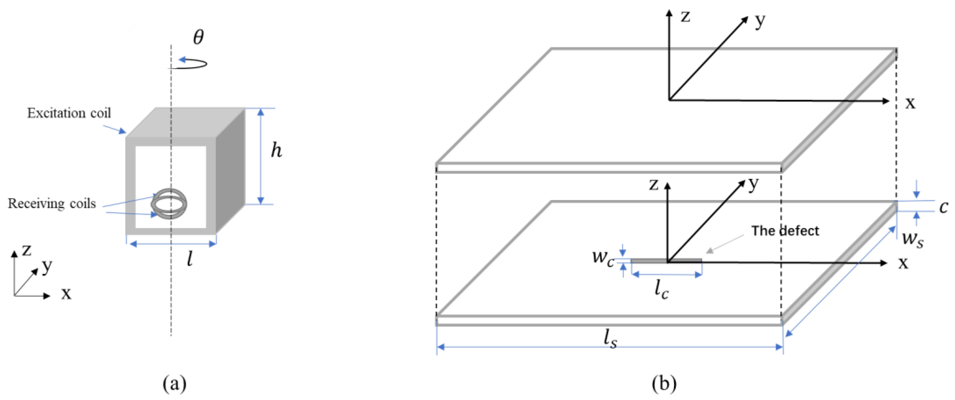
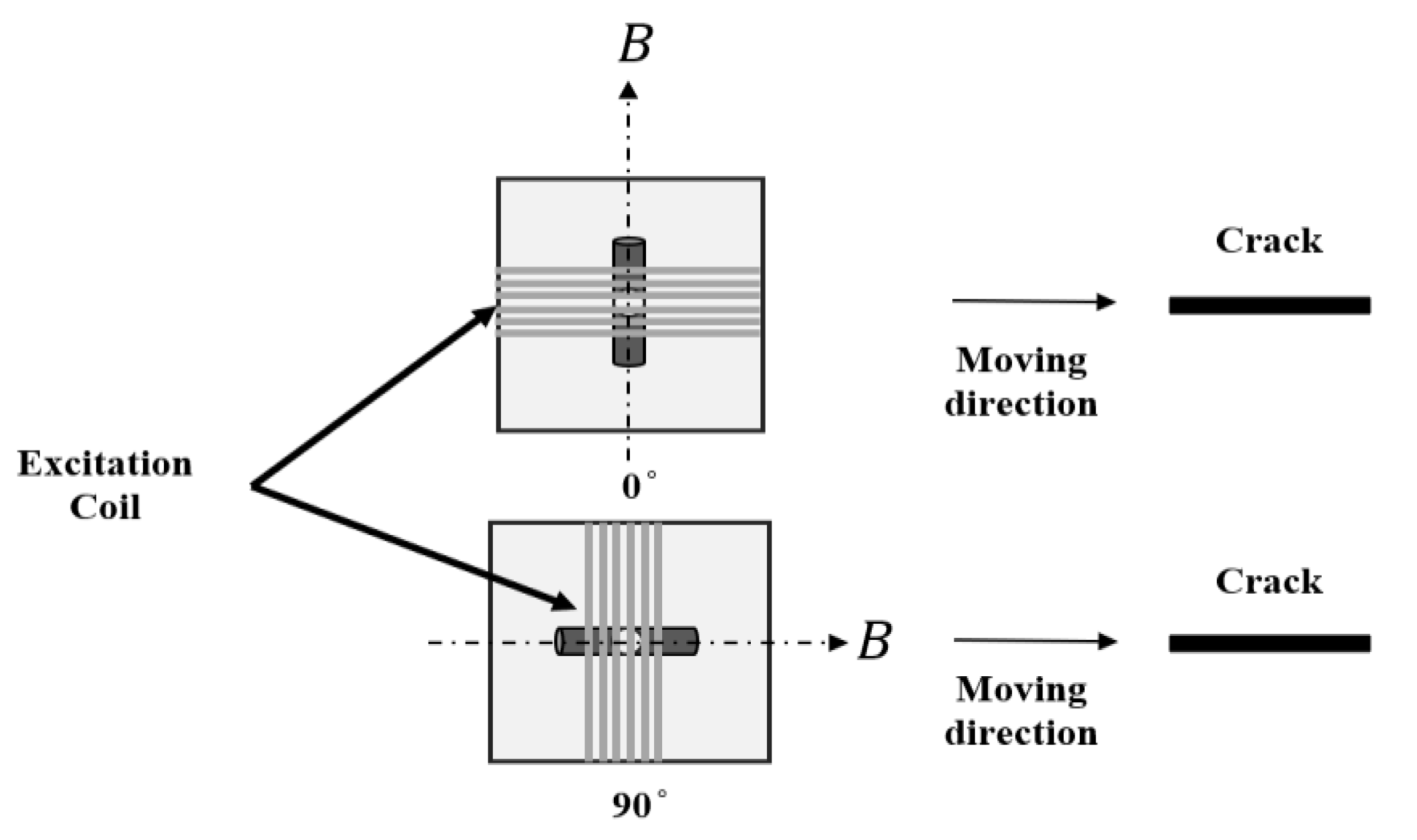
2.2. Simulation Models
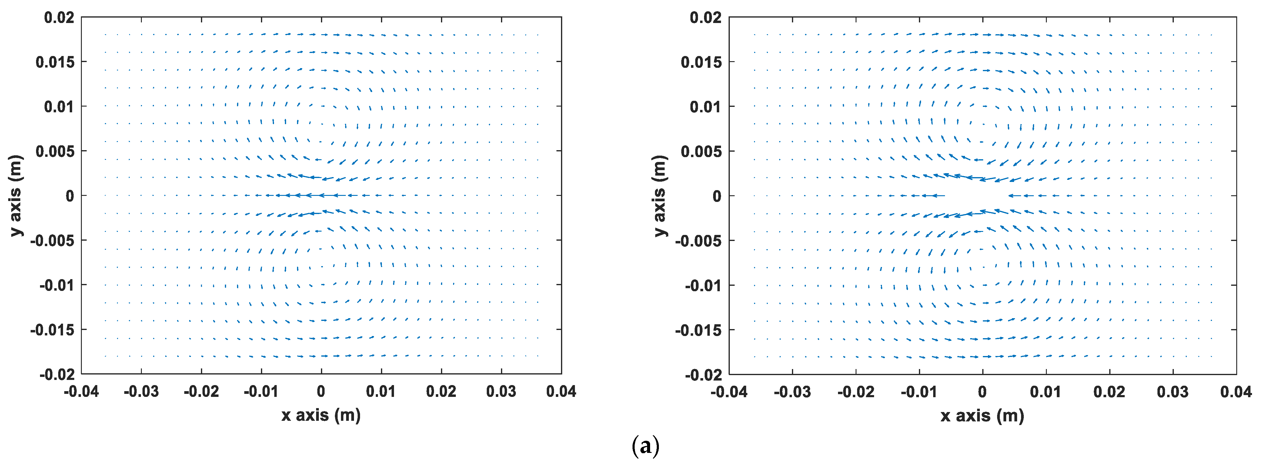
2.3. Eddy Currents around Cracks Using the FEM Solver
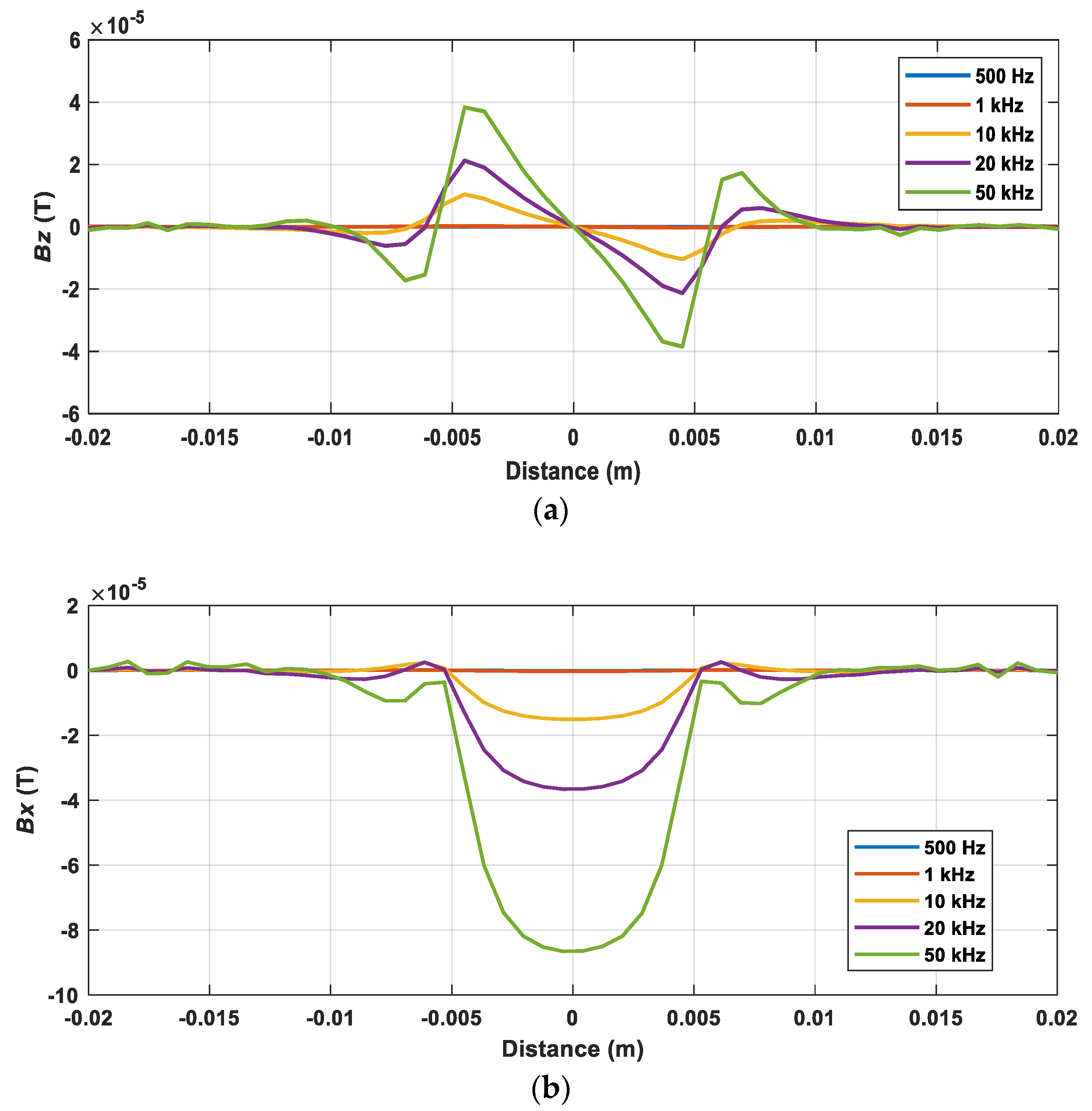
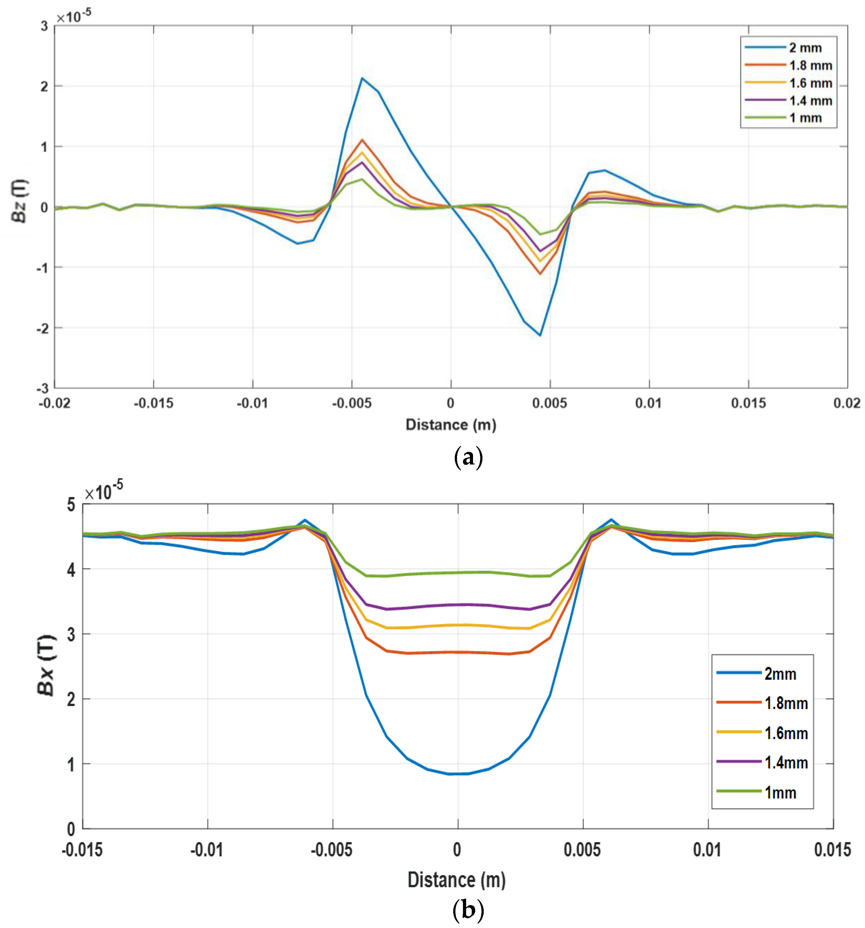
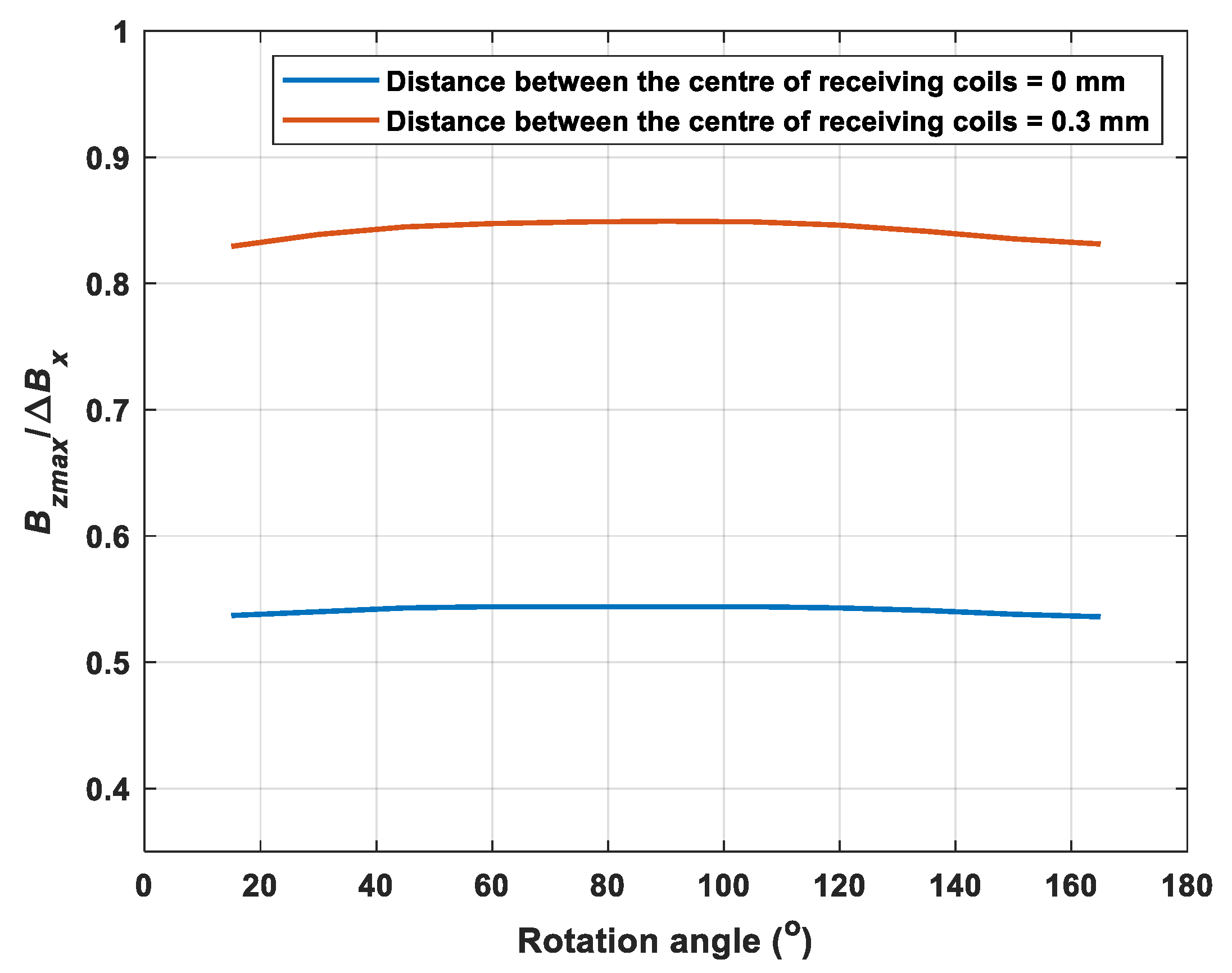
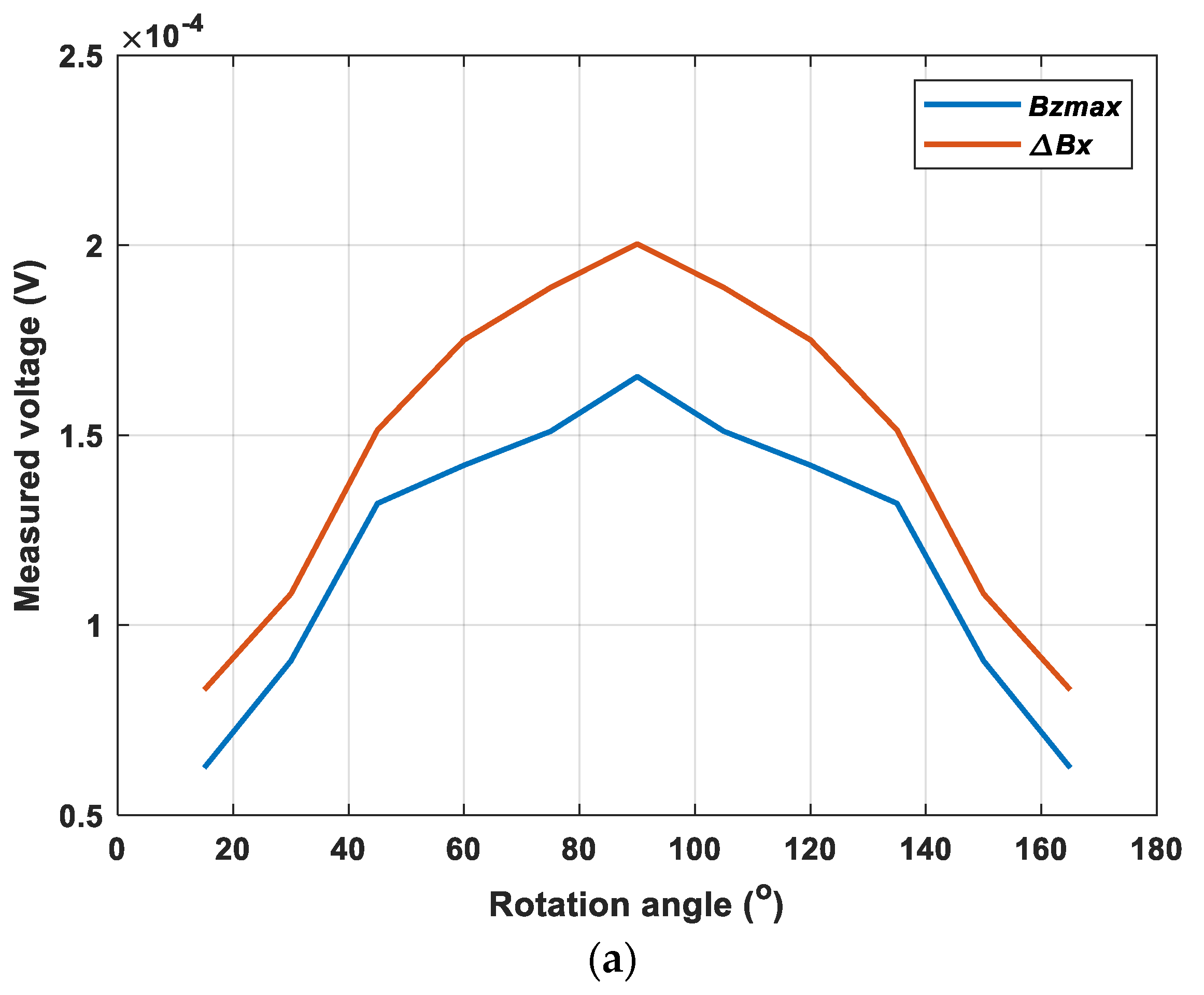
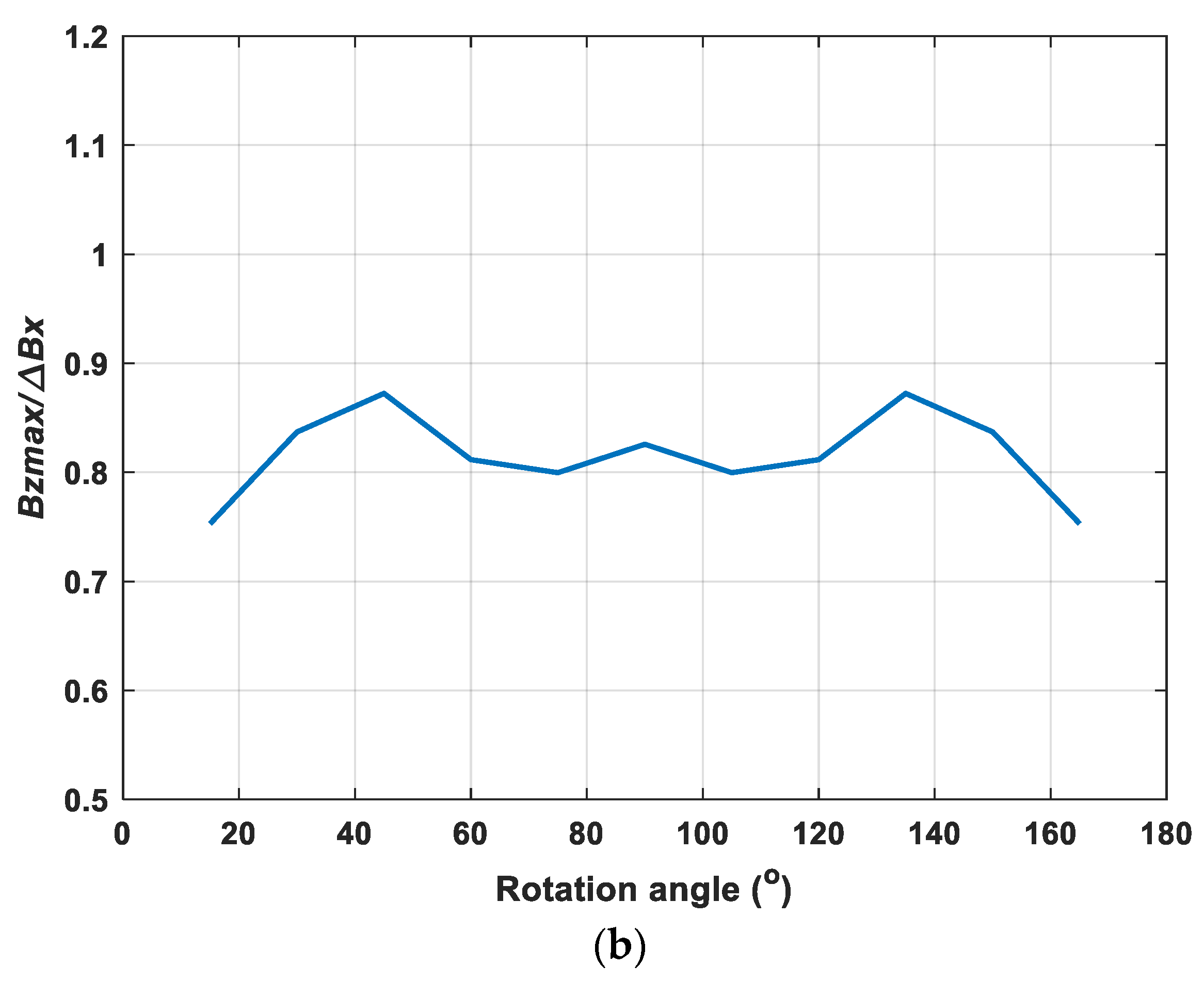
2.4. Coil Angle-Immune Feature on Crack Detection Using the Rotary Sensor Probe
3. Experiments
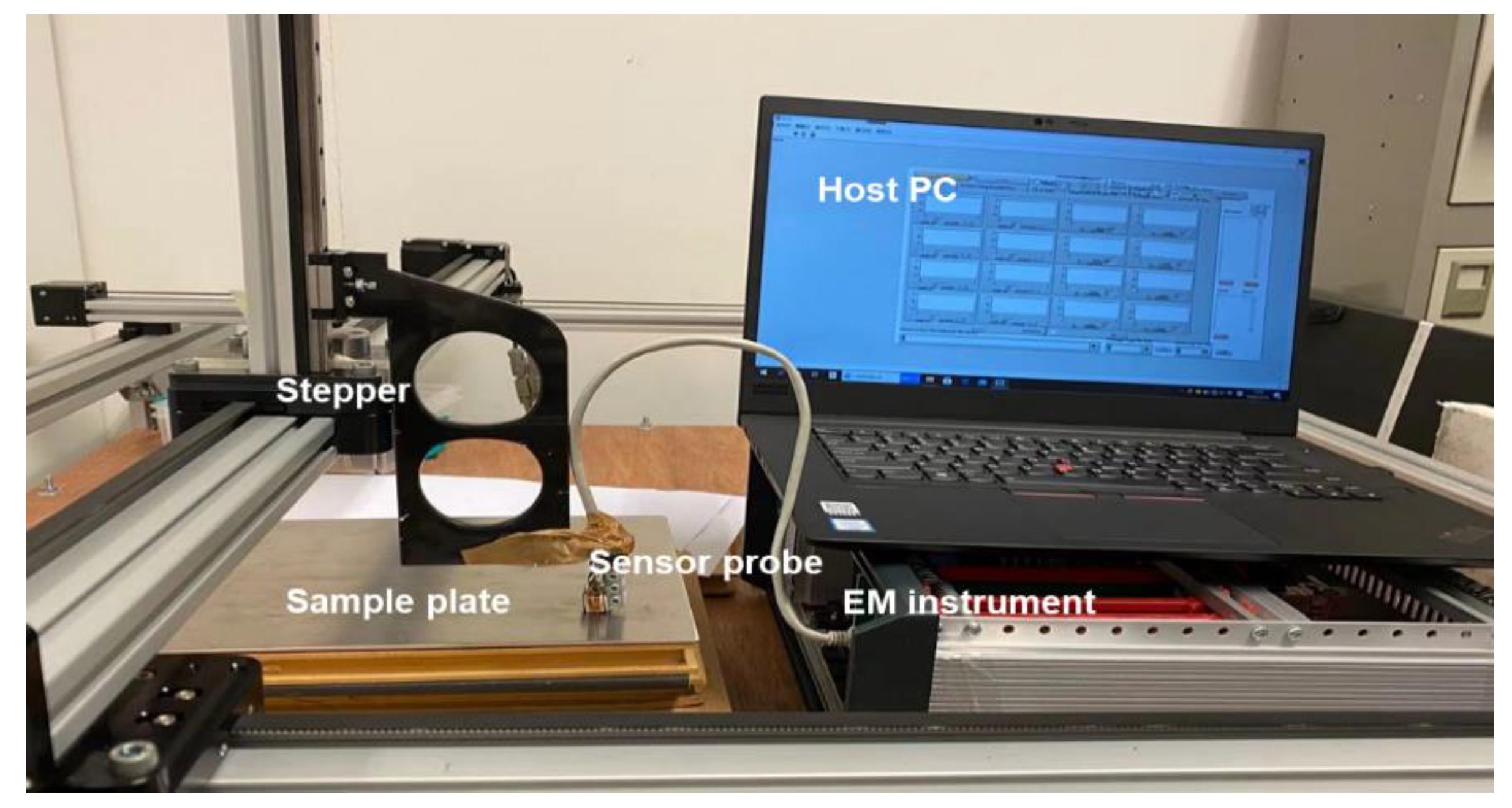
3.1. Experimental Setup
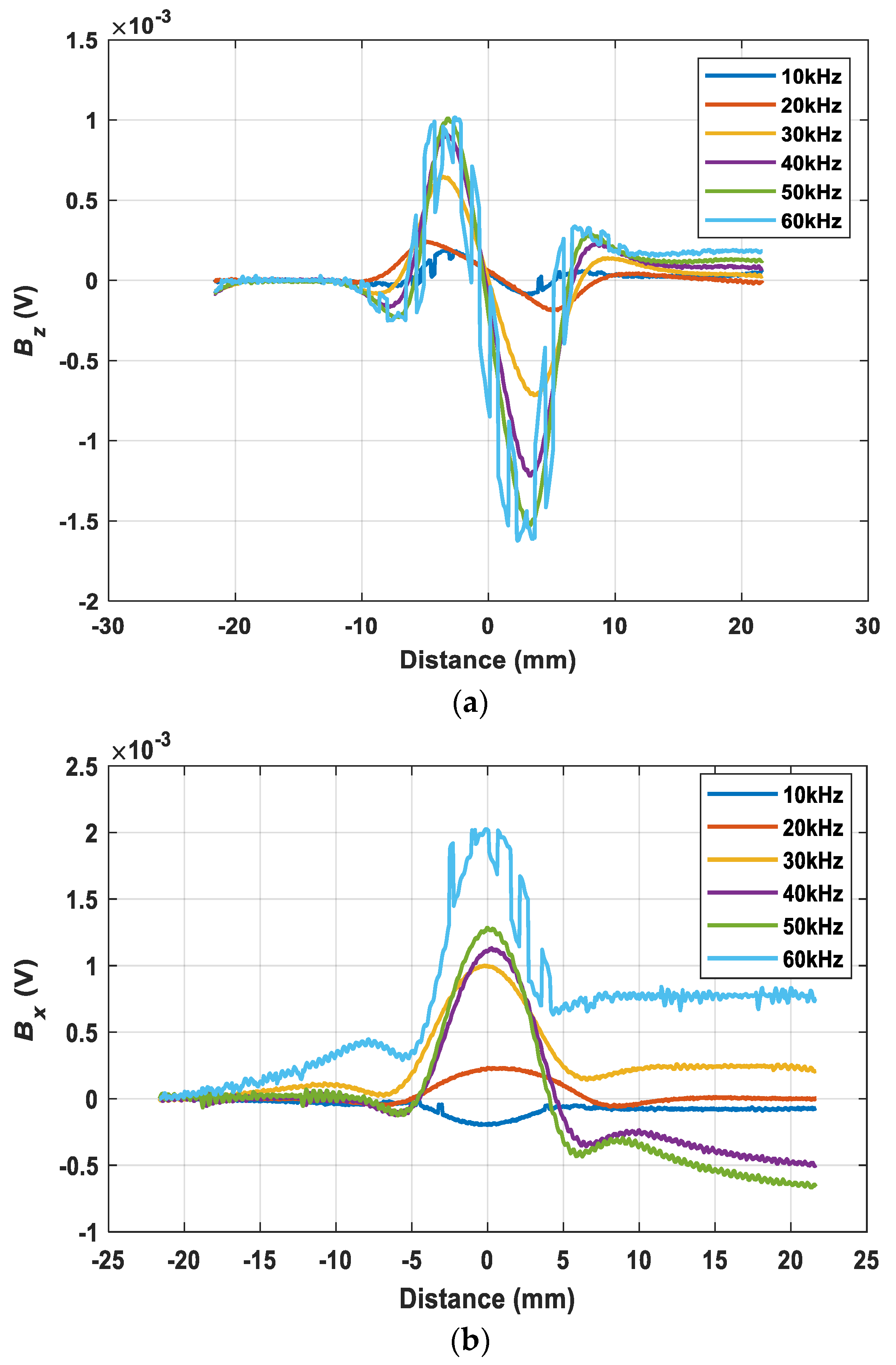
3.2. Coil-Crack Angle Insensitive Feature
4. Conclusions
Author Contributions
Funding
Institutional Review Board Statement
Informed Consent Statement
Data Availability Statement
Conflicts of Interest
References
- Ye, C.; Rosell, A.; Haq, M.; Stitt, E.; Udpa, L.; Udpa, S. EC probe with orthogonal excitation coils and TMR sensor for CFRP inspection. Int. J. Appl. Electromagn. Mech. 2019, 59, 1247–1255. [Google Scholar] [CrossRef]
- Xu, Z.; Wang, X.; Deng, Y. Rotating focused field Eddy-current sensing for arbitrary orientation defects detection in carbon steel. Sensors 2020, 20, 2345. [Google Scholar] [CrossRef] [Green Version]
- Ye, C.; Huang, Y.; Udpa, L.; Udpa, S.S. Novel rotating current probe with GMR array sensors for steam generate tube inspection. IEEE Sens. J. 2016, 16, 4995–5002. [Google Scholar] [CrossRef]
- Yang, G.; Dib, G.; Udpa, L.; Tamburrino, A.; Udpa, S.S. Rotating field EC-GMR sensor for crack detection at fastener site in layered structures. IEEE Sens. J. 2014, 15, 463–470. [Google Scholar] [CrossRef]
- Knight, M.J.; Brennan, F.P.; Dover, W.D. Effect of residual stress on ACFM crack measurements in drill collar threaded connections. NDT&E Int. 2004, 37, 337–343. [Google Scholar]
- Low, C.K.; Wong, B.S. Defect evaluation using the alternating current field measurement technique. Insight-Non-Destr. Test. Cond. Monit. 2004, 46, 598–605. [Google Scholar] [CrossRef]
- Blakeley, B.; Lugg, M. ACFM: Application of ACFM for inspection through metal coatings. Insight-Non-Destr. Test. Cond. Monit. 2010, 52, 310–315. [Google Scholar] [CrossRef]
- Raine, G.A.; Smith, N. NDT of on and offshore oil and gas installations using the alternating current field measurement (ACFM) technique. Mater. Eval. 1996, 54, 461–465. [Google Scholar]
- Lugg, M.; Topp, D. Recent developments and applications of the ACFM inspection method and ACSM stress measurement method. In Proceedings of the ECNDT, Berlin, Germany, 25–29 September 2006; NDT.net: Bad Breisig, Germany, 2006. [Google Scholar]
- Raine, A.; Lugg, M. A review of the alternating current field measurement inspection technique. Sens. Rev. 1999, 19, 207–213. [Google Scholar] [CrossRef] [Green Version]
- Gaynor, T.; Roberts, D.; Homan, E.; Dover, W. Reduction in fatigue failures through crack detection by alternating current field measurement. In Proceedings of the IADC/SPE Drilling Conference, New Orleans, LA, USA, 12–15 March 1996. [Google Scholar] [CrossRef]
- Noroozi, A.; Hasanzadeh, R.P.R.; Ravan, M. A fuzzy learning approach for identification of arbitrary crack profiles using ACFM technique. IEEE Trans. Magn. 2013, 49, 5016–5027. [Google Scholar] [CrossRef]
- Howitt, M. Bombardier brings ACFM into the rail industry. Insight 2002, 44, 379–382. [Google Scholar]
- Shen, J. Responses of Alternating Current Field Measurement (ACFM) to Rolling Contact Fatigue (RCF) Cracks in Railway Rails. Ph.D. Thesis, University of Warwick, Coventry, UK, 2017. [Google Scholar]
- Dover, W.D.; Collins, R.; Michael, D.H. Review of developments in ACPD and ACFM. Br. J. Non-Destr. Test. 1991, 33, 121–127. [Google Scholar]
- Yin, W.; Lu, M.; Yin, L.; Zhao, Q.; Meng, X.; Zhang, Z.; Peyton, A. Acceleration of eddy current computation for scanning probes. Insight-Non-Destr. Test. Cond. Monit. 2018, 60, 547–555. [Google Scholar] [CrossRef]
- Lu, M.; Peyton, A.; Yin, W. Acceleration of frequency sweeping in eddy-current computation. IEEE Trans. Magn. 2017, 53, 1–8. [Google Scholar] [CrossRef] [Green Version]
- Huang, R.; Lu, M.; Peyton, A.; Yin, W. A novel perturbed matrix inversion based method for the acceleration of finite element analysis in crack-scanning eddy current NDT. IEEE Access 2020, 8, 12438–12444. [Google Scholar] [CrossRef]
- Mirshekar-Syahkal, D.; Mostafavi, R.F. 1-D probe array for ACFM inspection of large metal plates. IEEE Trans. Instrum. Meas. 2002, 51, 374–382. [Google Scholar] [CrossRef]
- Li, W.; Yuan, X.; Chen, G.; Yin, X.; Ge, J. A feed-through ACFM probe with sensor array for pipe string cracks inspection. NDT&E Int. 2014, 67, 17–23. [Google Scholar]
- Ren, S.-K.; Zhu, Z.-B.; Lin, T.-H.; Song, K.; Ren, J.-L. Design for the acfm sensor and the signal processing based on wavelet de-noise. In Proceedings of the 2009 2nd International Congress on Image and Signal, Processing, Tianjin, China, 17–19 October 2009; pp. 1–4. [Google Scholar]
- Ravan, M.; Sadeghi, S.H.H.; Moini, R. Neural network approach for determination of fatigue crack depth profile in a metal, using alternating current field measurement data. IET Sci. Meas. Technol. 2007, 2, 32–38. [Google Scholar] [CrossRef]
- Sinha, S.K.; Fieguth, P.W. Neuro-fuzzy network for the classification of buried pipe defects. Autom. Constr. 2006, 15, 73–83. [Google Scholar] [CrossRef]
- Pawar, P.M.; Ganguli, R. Matrix crack detection in thin-walled composite beam using genetic fuzzy system. J. Intell. Mater. Syst. Struct. 2005, 16, 395–409. [Google Scholar] [CrossRef]
- Gu, Z.; Chen, M.; Wang, C.; Zhuang, W. Static and Dynamic Analysis of a 6300 KN Cold Orbital Forging Machine. Processes 2021, 9, 7. [Google Scholar] [CrossRef]
- Huang, R.; Lu, M.; Chen, Z.; Shao, Y.; Hu, G.; Peyton, A.; Yin, W. A novel acceleration method for eddy current crack computation using finite element analysis. NDT&E Int. 2021. under review. [Google Scholar]
- Xu, H.; Lu, M.; Avila, J.R.S.; Zhao, Q.; Zhou, F.; Meng, X.; Yin, W. Imaging a weld cross-section using a novel frequency feature in multi-frequency eddy current testing. Insight-Non-Destr. Test. Cond. Monit. 2019, 61, 738–743. [Google Scholar] [CrossRef]
- Avila, J.R.S.; Chen, Z.; Xu, H.; Yin, W. A multi-frequency NDT system for imaging and detection of cracks. In Proceedings of the 2018 IEEE International Symposium on Circuits and Systems (ISCAS), Florence, Italy, 27–30 May 2018; pp. 1–4. [Google Scholar]


| Values | |
|---|---|
| Height of excitation coil (mm) | 3 |
| Length of excitation coil (mm) | 4 |
| Turns of excitation coil | 5 |
| Radius of receiving coils (mm) | 0.5 |
| Turns of receiving coils | 1 |
| Lift-off (mm) | 0.5 |
| Width of the sample plate (mm) | 75 |
| Length of the sample plate (mm) | 40 |
| Thickness of the sample plate (mm) | 2 |
| Width of the crack (mm) | 10 |
| Length of the crack (mm) | 0.25 |
| Conductivity of the sample plate (MS/m) | 1.4 |
| Excitation coil | Length (mm) | 12 |
| Height (mm) | 10 | |
| Turns | 20 | |
| Receiving coil | Radius (mm) | 0.8 |
| Turns | 200 | |
| Lift-off (mm) | 1.5 | |
| Excitation frequency (kHz) | 20 | |
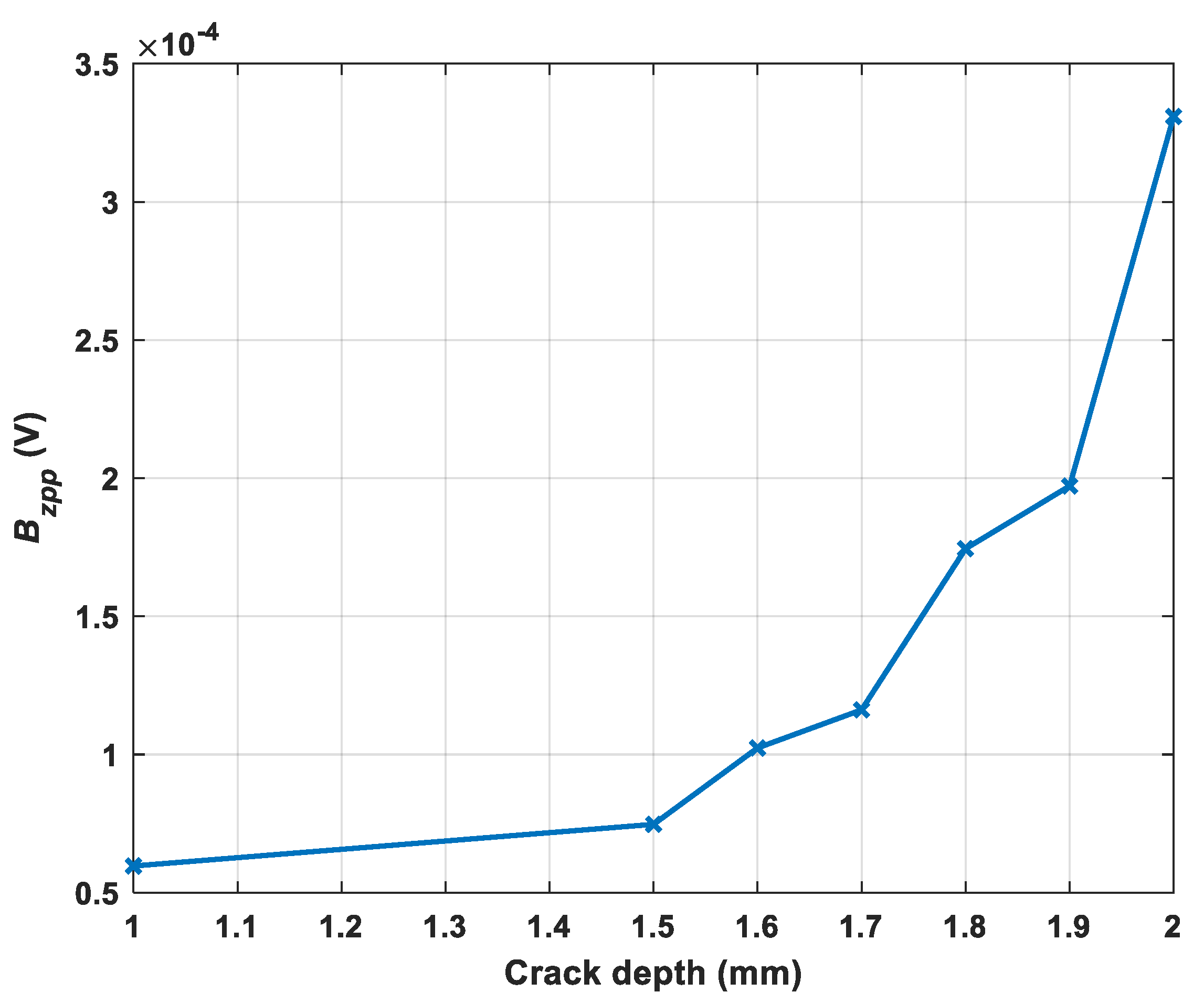
| Crack depth (mm) | 0.1:0.1:2 | |
Publisher’s Note: MDPI stays neutral with regard to jurisdictional claims in published maps and institutional affiliations. |
© 2021 by the authors. Licensee MDPI, Basel, Switzerland. This article is an open access article distributed under the terms and conditions of the Creative Commons Attribution (CC BY) license (https://creativecommons.org/licenses/by/4.0/).
Share and Cite
Huang, R.; Lu, M.; Chen, Z.; Yin, W. Reduction of Coil-Crack Angle Sensitivity Effect Using a Novel Flux Feature of ACFM Technique. Sensors 2022, 22, 201. https://doi.org/10.3390/s22010201
Huang R, Lu M, Chen Z, Yin W. Reduction of Coil-Crack Angle Sensitivity Effect Using a Novel Flux Feature of ACFM Technique. Sensors. 2022; 22(1):201. https://doi.org/10.3390/s22010201
Chicago/Turabian StyleHuang, Ruochen, Mingyang Lu, Ziqi Chen, and Wuliang Yin. 2022. "Reduction of Coil-Crack Angle Sensitivity Effect Using a Novel Flux Feature of ACFM Technique" Sensors 22, no. 1: 201. https://doi.org/10.3390/s22010201
APA StyleHuang, R., Lu, M., Chen, Z., & Yin, W. (2022). Reduction of Coil-Crack Angle Sensitivity Effect Using a Novel Flux Feature of ACFM Technique. Sensors, 22(1), 201. https://doi.org/10.3390/s22010201