Article

Dynamic Point Cloud Compression Based on Projections, Surface Reconstruction and Video Compression

1
Department of Electrical Engineering, University North, 104. Brigade 3, 42000 Varaždin, Croatia
2
Department of Electrical Engineering and Computing, University of Dubrovnik, Cira Carica 4, 20000 Dubrovnik, Croatia
3
Department of Informatics VII—Robotics and Telematics, Julius-Maximilians-University Würzburg, 97074 Würzburg, Germany
*
Author to whom correspondence should be addressed.
Sensors 2022, 22(1), 197; https://doi.org/10.3390/s22010197
Submission received: 26 September 2021 / Revised: 11 December 2021 / Accepted: 14 December 2021 / Published: 28 December 2021
(This article belongs to the Special Issue 3D Reconstruction with RGB-D Sensors)

Abstract

:
In this paper we will present a new dynamic point cloud compression based on different projection types and bit depth, combined with the surface reconstruction algorithm and video compression for obtained geometry and texture maps. Texture maps have been compressed after creating Voronoi diagrams. Used video compression is specific for geometry (FFV1) and texture (H.265/HEVC). Decompressed point clouds are reconstructed using a Poisson surface reconstruction algorithm. Comparison with the original point clouds was performed using point-to-point and point-to-plane measures. Comprehensive experiments show better performance for some projection maps: cylindrical, Miller and Mercator projections.

1. Introduction

A point cloud represents a set of discrete points in a given coordinate system, usually in a three-dimensional Cartesian system. It can represent different objects, urban settings and landscapes, or any other physical entities in different use cases such as: computer graphics and gaming, virtual reality, 3D content creation, medical applications, construction and manufacturing, consumer and retail, cultural heritage, remote sensing, autonomous vehicles, surveillance etc. [1]. Point clouds, together with light fields and digital holography are described as plenoptic representations of the visual scene, that are used in many immersive applications [2]. Point cloud processing algorithms can be considered in different scenarios, such as acquisition [3,4], coding and transmission [5,6] and (re)presentation and display [7,8].
Due to the data size of a static and dynamic point cloud, it is important to define efficient compression techniques for storage and compression. In this paper, we will present a dynamic point cloud compression that can be used in a point cloud transmission system. A basic overview has been presented in [9], while in [10] several static point clouds (with different sizes, e.g., number of points) have been compressed and decompressed using the equirectangular projection with a similar number of points as in the other used octree-based compression. In this paper we will present a comprehensive comparison of 10 different projection types, combined with the video compression algorithms for geometry and texture, and finally test surface reconstruction algorithms to fill the holes present after the lossy point cloud decompression process.
The structure of this article is as follows. Section 2 presents a related overview of point cloud compression algorithms. Section 3 presents different projection types that are used for projecting 3D point cloud to the image and vice versa. Section 4 describes the creation of the panorama image from a point cloud and how to recreate a point cloud from a panorama image. Section 5 gives the results from different projection types described in the previous section, using different objective quality measures and finally Section 6 gives the conclusions.

2. Related Work

Several static and dynamic point cloud coding solutions have been proposed recently. In [11] the authors describe an efficient octree implementation that is used to store, compress or visualize large point clouds. Storing is done without loss of precision, while reducing the size of a point cloud to half the original size. Also, 3D scan matching has been tested using the proposed method, by implementing the octree for nearest neighbor search (NNS) algorithm. The Random Sample Consensus (RANSAC) algorithm is also sped up by using the octree data structure. In the related work [12], shape registration algorithms have been compared using different NNS strategies, with the octree-based method being one of them. The Octree implementation (with arbitrarily chosen octree depth) is given in the “3DTK—The 3D Toolkit” [13].
Different from octree-based compression, in [14] the authors presented a point cloud compression algorithm based on projections. Different panorama generation methods have been tested, using several projection types: equirectangular, cylindrical, Mercator, rectilinear, Pannini, stereographic and Albers equal-area conic projections. It is shown that the reduced point clouds are useful for feature based registration on panorama images. In [15] point cloud compression scheme is proposed using panorama generated images and an equirectangular projection type. Range, color and reflectance information is encoded for each point, by using 24 bits for range (and storing it in an RGB image), 24 bits for color and 8 bits for reflectance. Also, lossless and lossy compression methods have been tested for obtained panorama images. In the case of lossy JPEG compression, an additional method is needed to remove artefacts from the decompressed point cloud.
Similarily, MPEG recently proposed two new point cloud compression codecs, named G-PCC (Geometry based Point Cloud Compression) codec [16] and V-PCC (Video based Point Cloud Compression) codec [17]. The G-PCC was created by merging two previously defined codecs, the L-PCC (LIDAR point cloud compression for dynamic point clouds) and the S-PCC (Surface point cloud compression for for static point clouds). Currently, G-PCC supports only intra prediction, so it does not use temporal redundancies. G-PCC compresses point clouds directly in 3D space. Currently, lossless mode provides up to a 10:1 compression ratio, while in lossy mode it is possible to obtain up to a 35:1 compression ratio with acceptable quality. In the MPEG’s V-PCC codec, the basic idea is to project point cloud from 3D to 2D, so that 2D projections are encoded using existing 2D video encoders such as H.265/HEVC video compression [18]. The current V-PCC encoder compresses dynamic point cloud with a compression ratio up to 125:1, with acceptable quality. More details about G-PCC and V-PCC are given in [19,20]. A comprehensive overview of G-PCC and V-PCC rate-distortion coding performance can be also found in [21]. A quality evaluation study of point cloud codecs G-PCC and V-PCC is presented in [22], showing the superior compression performance of the MPEG V-PCC compared to the MPEG G-PCC, for the selected static contents.
Neural network based point cloud compression schemes have also been proposed recently. In [23], the authors present point cloud compression using neural networks for separate and joint compression of geometry and texture. Better results are obtained for geometry and competitive results for color coding at low bitrates, comparing with CWI-PCL, the MPEG anchor codec is presented in [24]. In the paper [25], authors presented a new method for static point cloud geometric compression. It is based on the learned convolutional transform and uniform quantization. Compared to the MPEG reference software, the proposed algorithm achieves on average 51.5% BD-Rate (Bjöntegaard Delta Rate) savings, using the Microsoft Upper Body dataset [26]. The updated algorithm is presented in [27]. In the paper [28] a learned point cloud geometry compression is proposed, utilizing deep neural network-based variational autoencoders. The proposed algorithm shows higher compression efficiency than that of MPEG’s G-PCC, having at least 60% BD-Rate savings, tested on several datasets. The updated algorithm is proposed in [29]. Similar to [27] authors in [30] present the deep-learning coding approach to static point cloud geometry coding where a voxelized input point cloud is divided into 3D coding blocks of a fixed size and only non-empty 3D blocks are coded. The encoder transforms the input data into latent representations with lower dimensionality forcing a network to extract important features. The autoencoder learns the transform and its inverse operation suitable for the target data compared to image-transform coding where the transform basis functions are fixed. Performance results show improvements over the PCL (Point Cloud Library) [31]. The proposed compression from [30] is improved in [32] by adding the variational autoencoder which captures structure information still present on latent features and therefore entropy coding model parameters can be estimated on the encoder side and replicated on the decoder side more accurately. More importantly the authors add the resolution scalability via interlaced sub-sampling which not only increases the number of decoded points but also gives a good point cloud quality from a subjective point of view. Furthermore, these authors proposed adaptive deep learning-based static point cloud geometry coding which can adapt to any generic point cloud content to maximize the RD performance [33]. The author in [34] presents an adversarial autoencoding strategy for voxelized point cloud geometry where the main idea is to code each point cloud element independently and to decode it using a lower resolution reconstruction as side information. The encoder generates hash bytes, and the decoder combines them with side information to reconstruct the original block. The reconstructed block can be classified with an adversarial discriminator which is a regularizer for the reconstruction process thus improving the coding performance. A neural network architecture using a predictive coding module at the decoder stage for bit-rate reduction of geometry only point clouds is described in [35]. In this approach a block can be encoded independently or predicted using its neighbors based on the quality of the reconstructed block and the local topology of the model. Alternative to the mentioned block-by-block processing approaches point based models are used. In [36] the authors create an architecture consisting of a pointnet-based encoder, an uniform quantizer, an entropy estimation block and a nonlinear synthesis transformation module and in [37] a hierarhical autoencoder with multiscale loss function is presented. These architectures are insufficient for the processing of large point cloud data. VoxelDNN was proposed in [38] which combines the octree and voxel domains. Inference in this lossless compression is slow, and the occupancy probabilities are predicted sequentially, voxel by voxel, while the improved MSVoxelDNN models voxel occupancy and achieves rate savings over G-PCC up to 17% on average [39]. One of the new methods is presented in [40] and it brings a solution that can be applied to both static and dynamic point cloud compression. It employs the voxel context based entropy model and for dynamic PC compression temporal dependency is exploited. In the work of [41] detachable learning-based residual coding solution is created where the residual module enhances the decoded model quality at the expense of added bitrate.

3. Projection Types and Their Description

In this section, we describe different projection types and their inverse solutions that is later used in the process of obtaining 2D image projection from point clouds. Several of them are adopted from [15,42,43]. For each projection type, example panorama images for the geometry and texture are created using the point cloud “longdress_vox10_1060.ply” from Longdress dynamic point cloud dataset [44].
A point cloud geometry is first transformed from a Cartesian to a spherical coordinate system. Afterwards, 2D geometry panorama image coordinates (row number x and column number y) are calculated from the angle information (longitude θ and latitude φ ), while the intensity (bit depth) of the 2D geometry panorama represents radius in spherical coordinates. An attribute panorama image, i.e., a 2D image representing color information in our case, is created by using the same row number x and column number y as for the geometry, with the same color as the point cloud point that it represents.

3.1. Lambert Azimuthal Equal-Area Projection

Transformation equations and the inverse formulas are given in Equations (1) and (2). φ 1 is the standard parallel, while θ 0 is the central longitude.
x = k cos φ sin ( θ θ 0 ) , y = k ( cos φ 1 sin φ sin φ 1 cos φ cos ( θ θ 0 ) ) , k = 2 1 + sin φ 1 sin φ + cos φ 1 cos φ cos ( θ θ 0 ) .
The inverse formulas are given in Equation (2):
θ = arctan x sin C ρ cos φ 1 cos C y sin φ 1 sin C + θ 0 , φ = arcsin cos C sin φ 1 + y sin C cos φ 1 ρ , ρ = x 2 + y 2 , C = 2 arcsin ρ 2 .
An example of panorama images is given in Figure 1.

3.2. Albers Equal-Area Conic Projection

Transformation equations and the inverse formulas are given in Equations (3) and (4). Usually, ( φ 0 , θ 0 ) = ( 0 , 0 ) , while φ 1 and φ 2 represent minimum and maximum latitude.
x = ρ sin ( N ( θ θ 0 ) ) , y = ρ 0 ρ cos ( N ( θ θ 0 ) ) ,
where:
N = 1 2 ( sin φ 1 + sin φ 2 ) , C = cos 2 φ 1 + 2 N sin φ 1 , ρ 0 = 1 N C 2 N sin φ 0 , ρ = 1 N C 2 N sin φ .
The inverse formulas are given in Equation (4):
θ = θ 0 + 1 N arctan x ρ 0 y , φ = arcsin C ( x 2 + ( ρ 0 y ) 2 ) N 2 2 N .
An example of panorama images is given in Figure 2.

3.3. Cylindrical Projection

Cylindrical projection is similar to the equirectangular projection, however vertical coordinate is tangent of the latitude. Transformation equations and the inverse formulas are given in Equations (5) and (6). Usually, ( φ 0 , θ 0 ) = ( 0 , 0 ) . Later in the experiments, we will “compress” all φ latitude angles before creating panorama images, i.e., multiply φ with 0.825, and “decompress” (divide by 0.825) after recreating point cloud. This is because tangent function is not defined for angles near ± 90 .
x = θ θ 0 , y = tan φ tan φ 0 .
The inverse formulas are given in Equation (6):
θ = x + θ 0 , ϕ = arctan ( y + tan φ 0 ) .
An example of panorama images is given in Figure 3.

3.4. Cylindrical Equal-Area Projection

Transformation equations and the inverse formulas are given in Equations (7) and (8). θ 0 is the standard longitude, while φ s is the standard latitude, e.g., for φ s = 0 it is called Lambert cylindrical equal-area projection.
x = ( θ θ 0 ) c o s φ s , y = sin φ cos φ s .
The inverse formulas are given in Equation (8):
θ = x cos φ s + θ 0 , φ = arcsin ( y cos φ s ) .
An example of panorama images is given in Figure 4.

3.5. Equidistant Cylindrical Projection

Transformation equations and the inverse formulas for equidistant cylindrical projection are given in Equations (9) and (10). An equirectangular projection, one of the most common projection types, is a type of cylindrical equidistant projection. Horizontal coordinate x in this projection type is the longitude θ , while the vertical coordinate y is the latitude φ . φ 1 represents standard parallels (north and south of the equator) where the scale of the projection is true. For ( φ 0 , θ 0 ) = ( 0 , 0 ) and cos φ 1 = 0 it is called the equirectangular projection, Equation (9).
x = ( θ θ 0 ) cos φ 1 , y = φ φ 0 .
The inverse formulas are given in Equation (10):
θ = x cos φ 1 + θ 0 , ϕ = y + ϕ 0 .
An example of panorama images is given in Figure 5.

3.6. Mercator Projection

Transformation equations and the inverse formulas are given in Equations (11) and (12). Problems may arise at latitudes φ near ± 90 . Usually, ( φ 0 , θ 0 ) = ( 0 , 0 ) . Similar to the cylindrical projection, later in the experiments we will “compress” all φ latitude angles, multiplying them with the factor 0.825, to create a panorama image (and “decompress”—divide them with the factor 0.825 to recreate point clouds).
x = θ θ 0 , y = ln tan φ + 1 cos φ y 0 , y 0 = ln tan φ 0 + 1 cos φ 0
The inverse formulas are given in Equation (12):
θ = x + θ 0 , φ = 2 arctan e y + y 0 π 2 .
An example of panorama images is given in Figure 6.

3.7. Miller Projection

The Miller projection is a modified Mercator projection. Transformation equations and the inverse formulas are given in Equations (13) and (14). Problems that may arise using the Mercator projection for latitudes ϕ near ± 90 are not present in the Miller projection. Usually, ( ϕ 0 , θ 0 ) = ( 0 , 0 ) .
x = θ θ 0 , y = 5 4 ln tan π 4 + 2 φ 5 y 0 . y 0 = 5 4 ln tan π 4 + 2 φ 0 5 .
The inverse formulas are given in Equation (14):
θ = x + θ 0 , φ = 5 2 arctan e 4 ( y + y 0 ) 5 5 π 8 .
An example of panorama images is given in Figure 7.

3.8. Rectilinear Projection

Transformation equations and the inverse formulas are given in Equations (15) and (16). θ 0 and φ 1 are the longitude and latitude of the center of the projection. It is recommended to use this projection for the horizontal and vertical angles of less than 120 . Therefore, the panorama has to be divided into smaller subsets, e.g., minimum 3 (later we will use 4). In addition, for greater vertical angles, all angles are scaled to fit in less than ± 90 . Later in the experiments, similar to the cylindrical and Mercator projections, we will “compress” and “decompress” all of the φ latitude angles, by multiplying and dividing them by 0.825.
x = cos φ sin ( θ θ 0 ) sin φ 1 sin φ + cos φ 1 cos φ cos ( θ θ 0 ) , y = cos φ 1 sin φ sin φ 1 cos φ cos ( θ θ 0 ) sin φ 1 sin φ + cos φ 1 cos φ cos ( θ θ 0 ) .
The inverse formulas are given in Equation (16):
θ = θ 0 + arctan x sin C ρ cos φ 1 cos C y sin φ 1 sin C , φ = arcsin cos C sin φ 1 + y sin C cos φ 1 ρ , ρ = x 2 + y 2 , C = arctan ρ .
An example of panorama images is given in Figure 8.

3.9. Pannini Projection

Transformation equations and the inverse formulas are given in Equations (17) and (18). θ 0 and φ 1 are the longitude and latitude of the center of the projection. Parameter d can be any non-negative number. For d = 0 we have a rectilinear projection, while d = 1 is the usual Pannini projection, used in the later experiments. It is recommended to use this projection for horizontal and vertical angles of less than 150 . Therefore, the panorama has to be divided into smaller subsets, e.g., minimum of 3 (later we will use 4). In addition, for greater vertical angles, all angles are scaled to fit in less than ± 90 . For this projection type, later in the experiments we will “compress” and “decompress” all φ latitude angles, multiplying and dividing them with the factor 0.825.
x = ( d + 1 ) sin ( θ θ 0 ) d + sin φ 1 tan φ + cos φ 1 cos ( θ θ 0 ) , y = ( d + 1 ) tan φ ( cos φ 1 sin φ 1 ( 1 tan φ ) cos ( θ θ 0 ) ) d + sin φ 1 tan φ + cos φ 1 cos ( θ θ 0 ) .
The inverse formulas are given in Equation (18):
A = y x cos φ 1 , B = tan φ 1 , C = A x sin φ 1 d 1 , D = B x sin φ 1 + x cos φ 1 , E = x d .
Finally we yield, Equation (19):
C sin ( θ θ 0 ) + D cos ( θ θ 0 ) = E θ = θ 0 + arccos E C 2 + D 2 + arctan C D φ = arctan ( A sin ( θ θ 0 ) + B cos ( θ θ 0 ) ) .
An example of panorama images is given in Figure 9.

3.10. Stereographic Projection

Transformation equations and the inverse formulas are given in Equations (20) and (21). θ 0 and φ 1 are the longitude and latitude of the center of the projection. It is advisable to use a 120 longitude, e.g., to divide the image into at least 3 subsets (later we will use 4).
x = 2 R cos φ sin ( θ θ 0 ) 1 + sin φ 1 sin φ + cos φ 1 cos φ cos ( θ θ 0 ) , y = 2 R ( cos φ 1 sin φ sin φ 1 cos φ cos ( θ θ 0 ) ) 1 + sin φ 1 sin φ + cos φ 1 cos φ cos ( θ θ 0 ) .
The inverse formulas are given in Equation (21):
θ = θ 0 + arctan x { i n C ρ cos φ 1 cos C y sin φ 1 sin C , φ = arcsin cos C sin φ 1 + y sin C cos φ 1 ρ , ρ = x 2 + y 2 , C = 2 arctan ρ 2 R .
An example of panorama images is given in Figure 10.

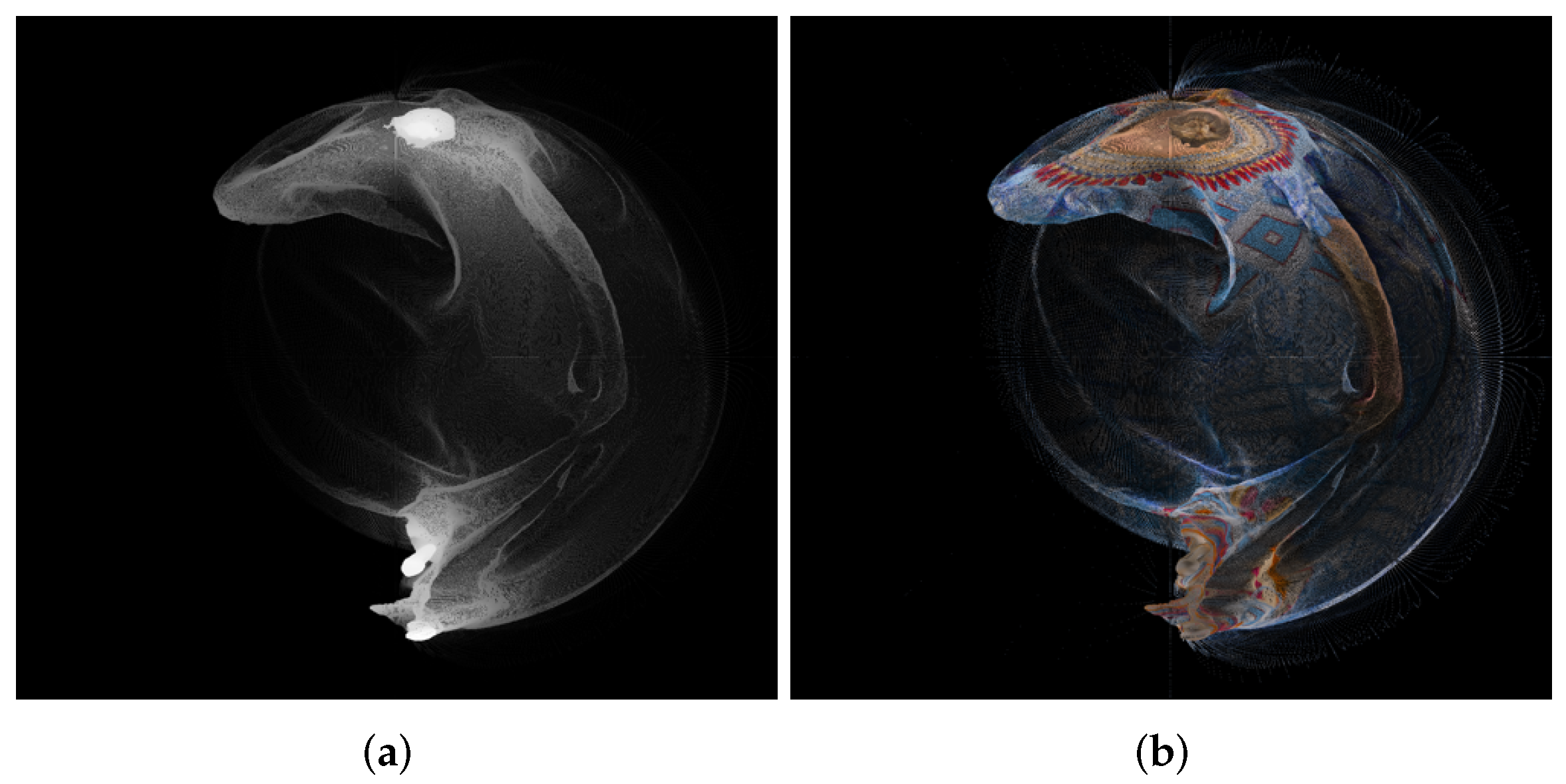
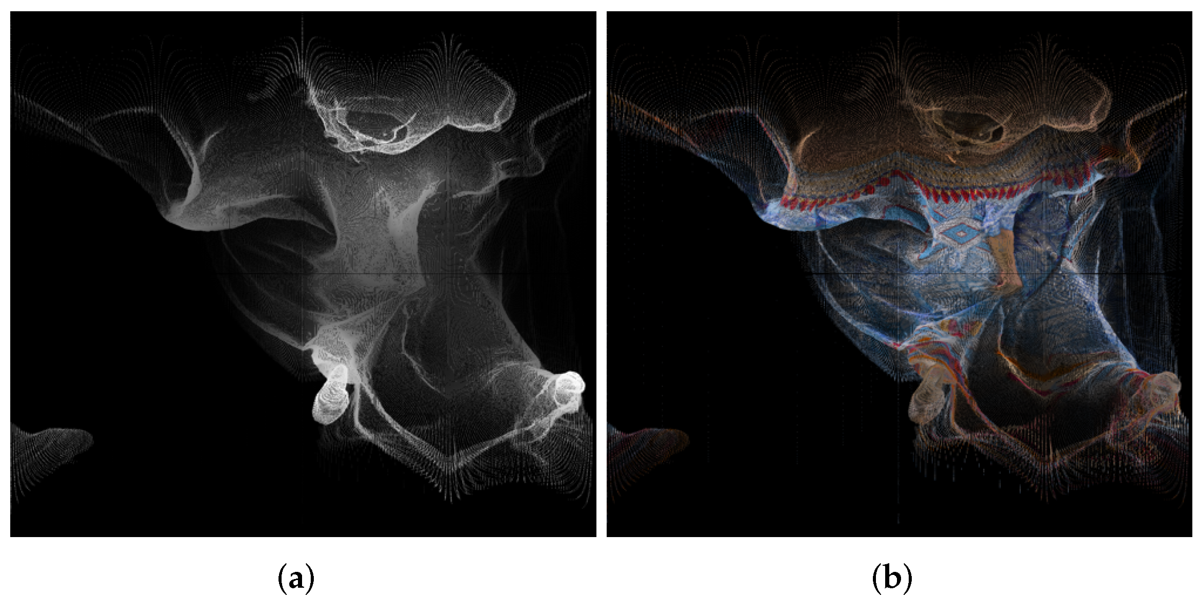
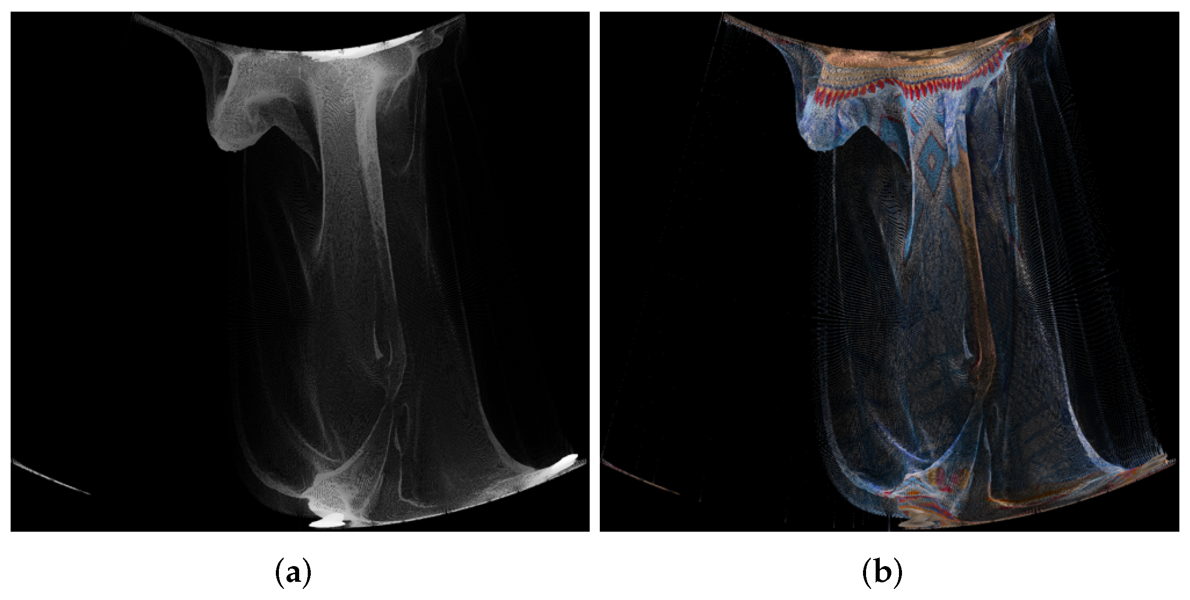
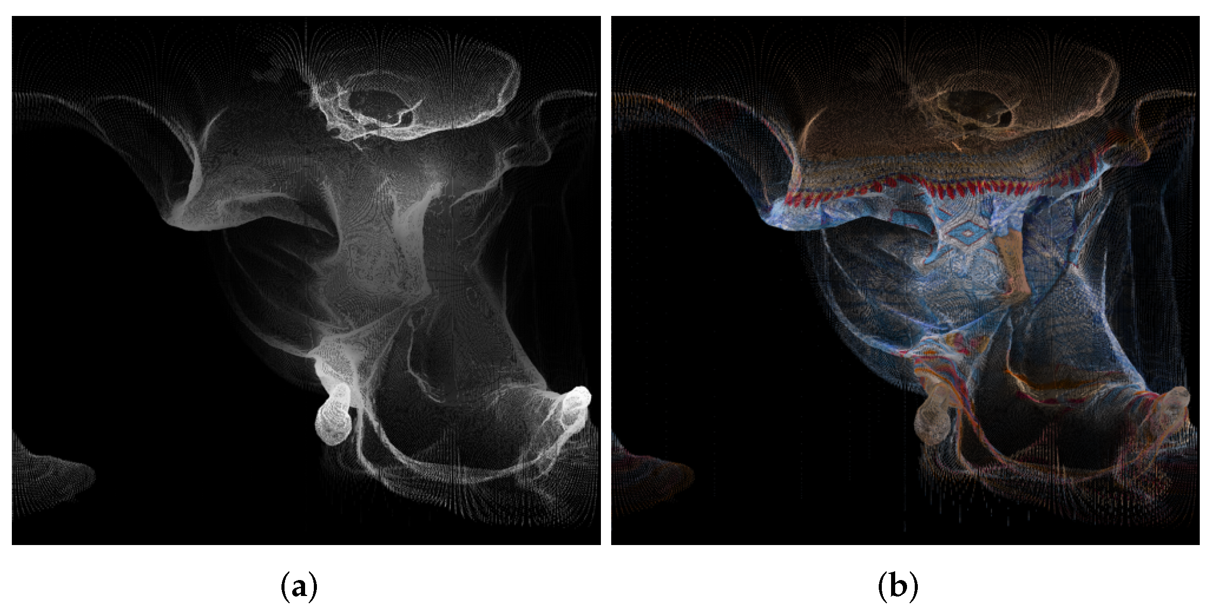
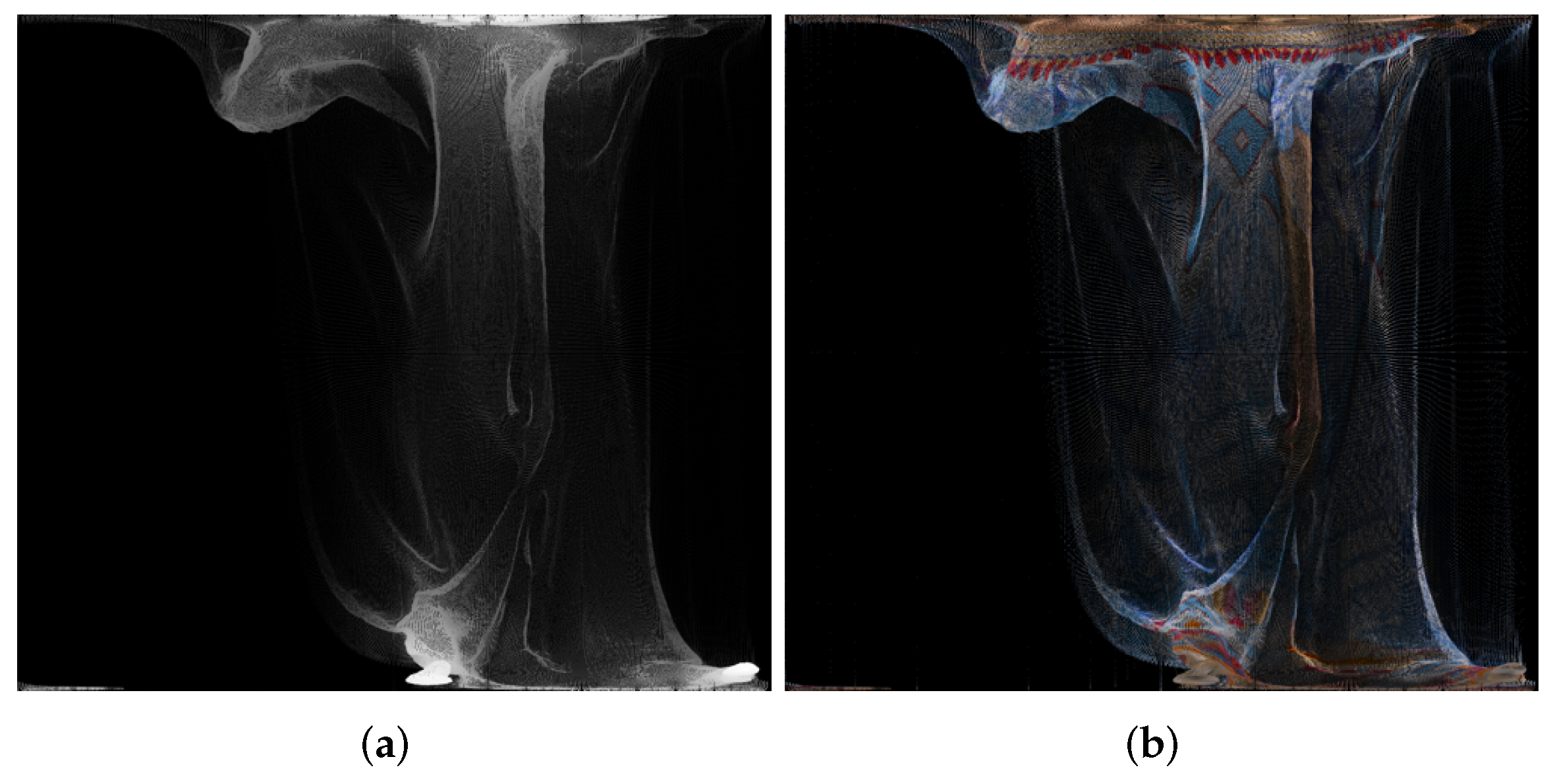
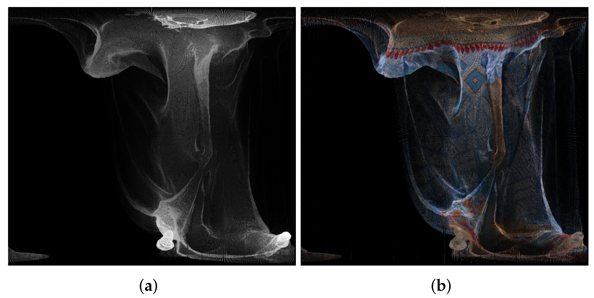
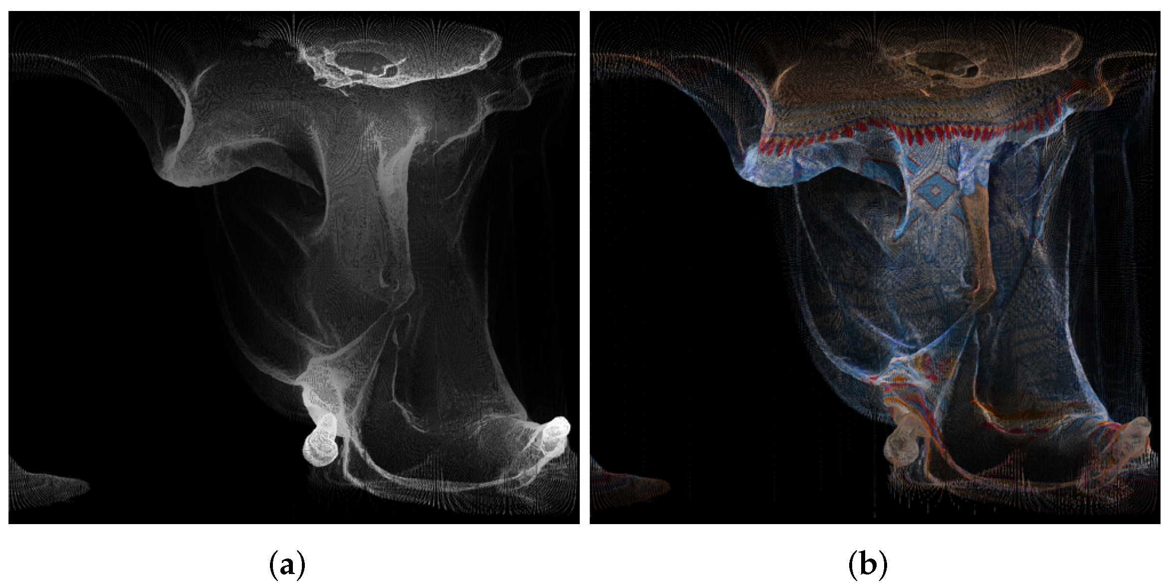
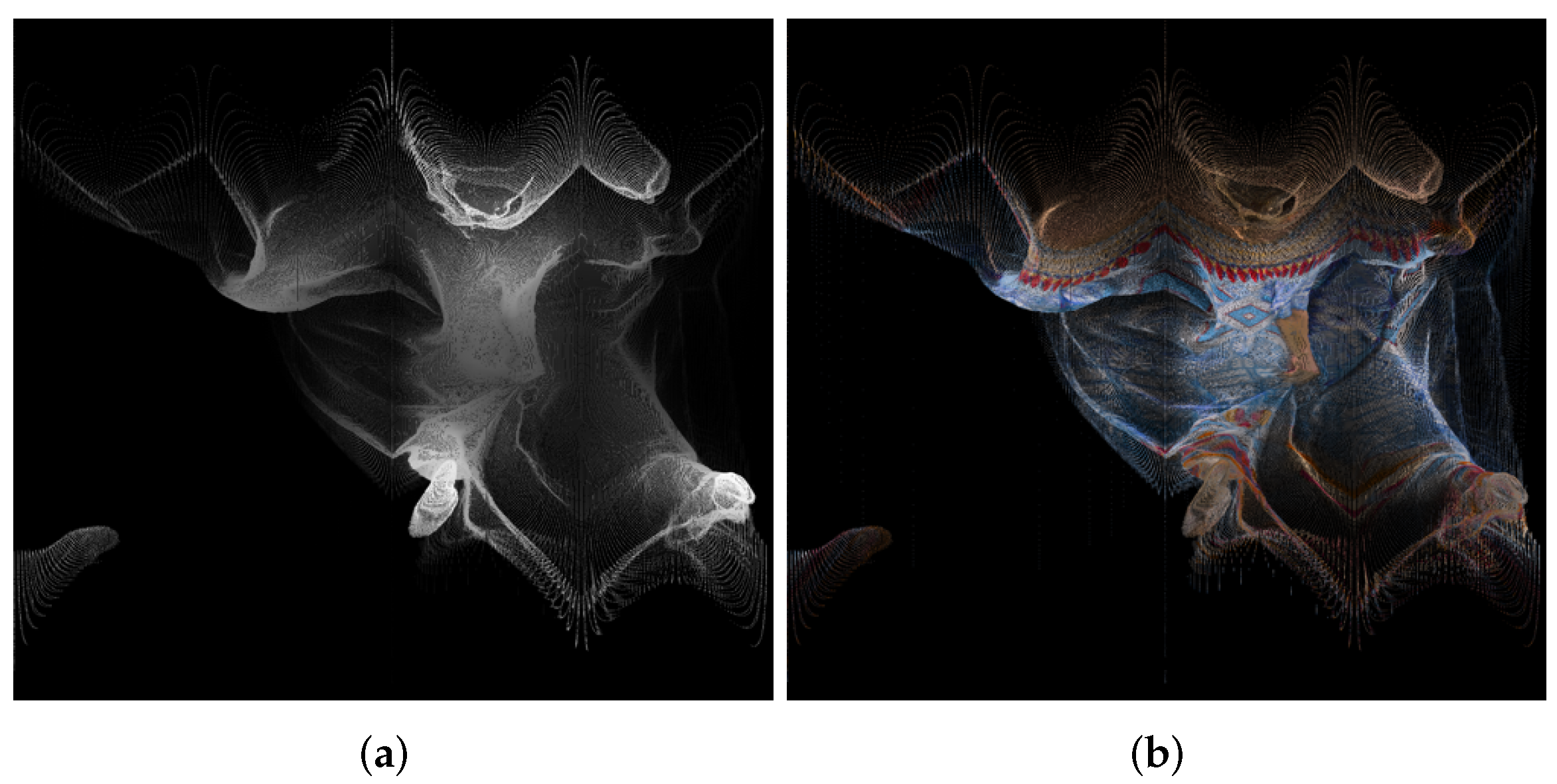
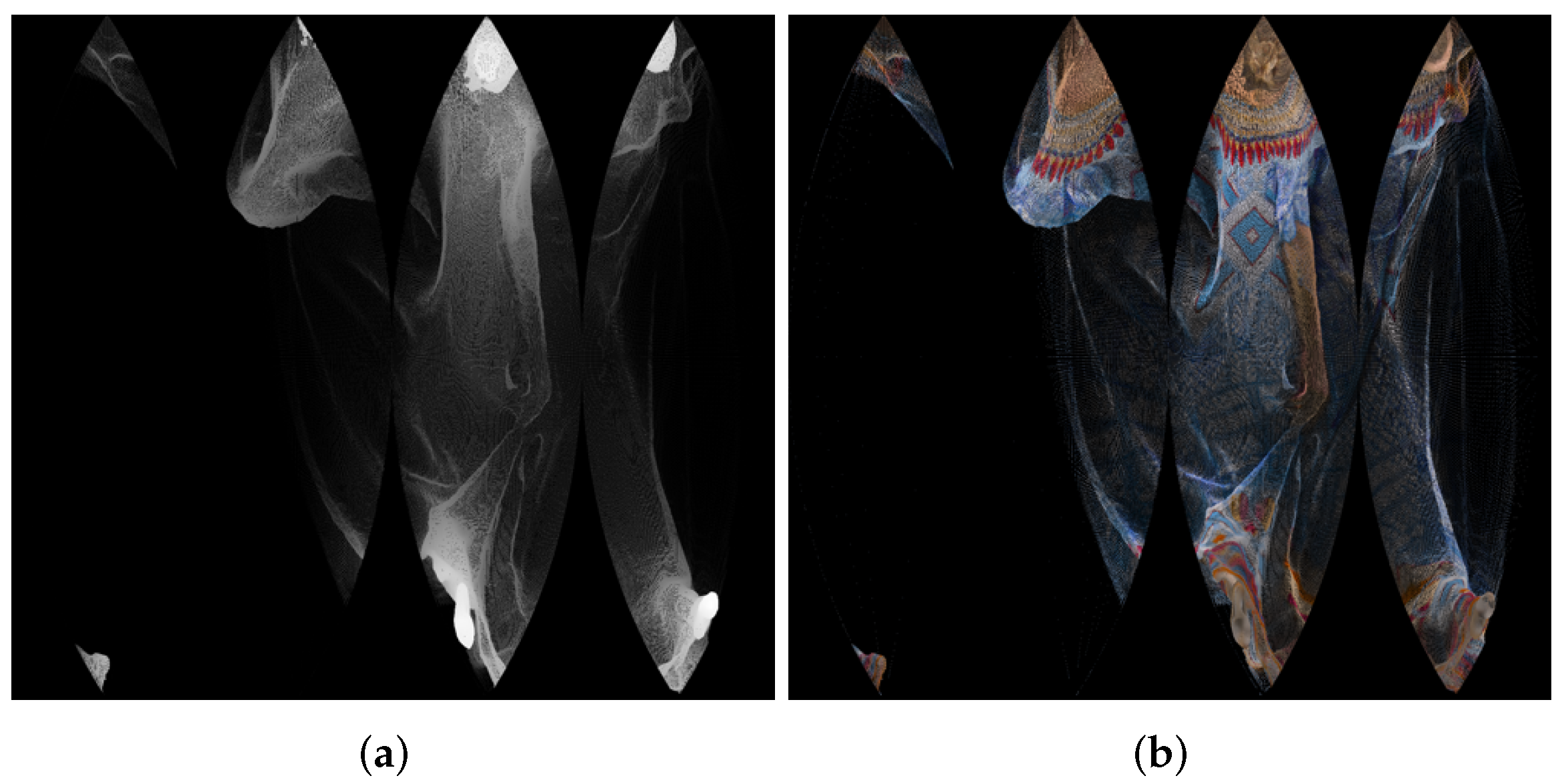
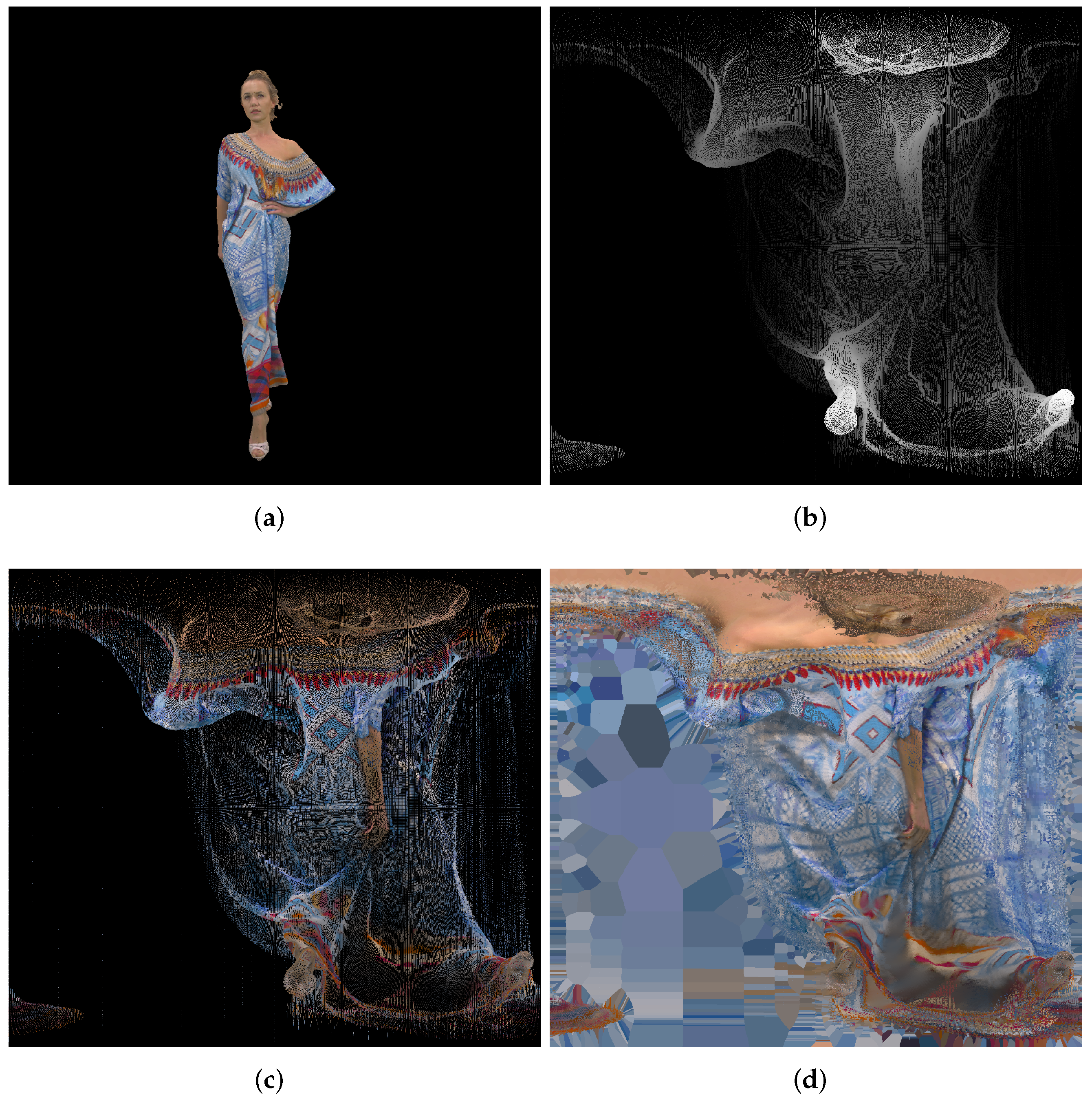
4. Creation of Panorama Images from Point Clouds and Recreation of Point Clouds

In this section we will describe how to calculate panorama images from point clouds, as well as how to recreate point clouds from obtained panorama images. Programs that were used are 3DTK toolkit [13], MeshLab [45], CloudCompare [46], FFmpeg [47] and MATLAB for scripts.
For this example, we will use the Miller projection, although any other projection described earlier can be used in a similar way. Also, we will use Longdress point cloud, first 20 frames [44]. This point cloud is a voxelized point cloud with a bounding box size of 1024 × 1024 × 1024, i.e., with 10-bit precision per each coordinate. Additionally, texture (color) for each point is represented with 24-bit RGB format, i.e., with 8 bits per color channel. Overall, 3 × 10 + 3 × 8 = 54 bits per point are used, in the ideal case; however, depending on the used format, even the binary format might occupy much more space, as we present later.
The input point cloud is read in MATLAB and an offset is added to all its points, so that the bounding box center is at (0, 0, 0). Afterwards, it is scaled so that the maximum distance between any point and the origin (0, 0, 0) does not exceed 2 b i t _ n u m 1 = 65 , 535 for a 16 bit panorama grayscale image, Equation (22).
scale _ factor = K · ( 2 bit _ num 1 ) max ( x x ( i ) 2 + y y ( i ) 2 + z z ( i ) 2 ) bit _ num = 16 ( in the later case , but could be also 24 for some other point clouds ) K = 0.01 ( due to the later scaling made by the 3 DTK toolkit ) i { 1 , , N } , N = number of points x x ( i ) , y y ( i ) , z z ( i ) are Cartesian coordinates of the point i
Both geometry and texture are represented using the same projection. In the case of geometry, we use 16 bit input grayscale .png for the later compression. However, approximately 9 bits may be enough for the tested point cloud: the maximum distance from the center is 512, before scaling, but the number may not be integer, so some precision loss may occur for the 9 bit representation. For larger point clouds, 24-bit representation may also be used, which is also implemented in the 3DTK toolkit, storing geometry in an RGB image [15]. In the case of texture, we additionally create a Voronoi diagram using OpenCV “distanceTransform” function and L2 norm (while creating the texture image in the 3DTK toolkit), Listing 1. A Voronoi diagram (tessellation, decomposition) is the partitioning of a plane with n points into convex polygons with exactly one generating point in each polygon and every point in a particular polygon being closer to its generating point than any other generating point [48]. By creating a “full” texture image, instead of originally sparse, additional video compression efficiency may be achieved later.
Listing 1. Voronoi diagram creation.
//create geometry and texture image using 3DTK
//get mask as the inverse of the existing pixels from~geometry
distanceTransform(mask, distance, labels, CV_DIST_L2,
CV_DIST_MASK_PRECISE, CV_DIST_LABEL_PIXEL);
//map labels to indices
std::vector<cv::Vec2i> label_to_index;
//reserve memory for faster push_back
label_to_index.reserve(sum(~mask)[0]);
for (int row = 0; row < mask.rows; ++row)
  for (int col = 0; col < mask.cols; ++col)
   if (mask.at<uchar>(row, col) == 0) //this pixel exist
    label_to_index.push_back(cv::Vec2i(row, col));
//create ``full’’ image
for (int row = 0; row < mask.rows; ++row) {
  for (int col = 0; col < mask.cols; ++col) {
   if (mask.at<uchar>(row, col) > 0) { //so this pixel needs to be filled
    colorImage.at<cv::Vec3b>(row,col)=
    cv::Vec3b(colorImage.at<cv::Vec3b>(label_to_index[labels.at<int>(row, col)])[0],
    colorImage.at<cv::Vec3b>(label_to_index[labels.at<int>(row, col)])[1],
    colorImage.at<cv::Vec3b>(label_to_index[labels.at<int>(row, col)])[2]);
  }
 }
}
The previously described algorithm is presented in Figure 11, for the tenth point cloud “longdress_vox10_1060.ply” and the Miller projection type. The projection area is set to be about 2,000,000 pixels. We define the ratio for the image size as the ratio between the first point cloud height and width, and again divided by π . In this example case, this ratio is 0.8968. Because later video compression expects frame width and height divisible by 8, we also round the final frame width and height to the nearest integer divisible by 8, Equation (23). Again, for the later video compression, all subsequent point clouds need to have the same frame size.
ratio = pc _ height π · pc _ width frame _ width = 8 · 1 8 · panorama _ area ratio frame _ height = 8 · 1 8 · frame _ width · ratio
After the first point cloud has been projected to 2D panorama, all the other subsequent point clouds are also projected to the panorama for geometry and texture with the same frame size as the first one. Also, geometry and texture are calculated in the same way as earlier described. Afterwards, we use FFmpeg and different video compressions for geometry and texture images. For texture, we use the x265 coder (H.265/HEVC) with lossy compression, while for geometry we use the FFV1 coder with lossless compression. For x265 (for texture) we use crf 17 (constant rate factor), pixel format rgb24, preset veryslow, while for FFV1 (for geometry) we use pixel format gray9le (depth of 9 bits per pixel), as well as gray10le (only in the case of Miller projection). For this case, the texture file size is 11.3 × 10 6 bytes and the geometry file size is 14 × 10 6 bytes, so overall size is 25.3 × 10 6 bytes.
Point cloud recreation is done by decompressing previously compressed video files, and afterwards using inverse formulas for used projection type, in this example Miller. For the color information, we use pixels from the panorama image for color (Voronoi diagram) that exist in panorama image for geometry. In the final step, we use several algorithms to oversample the original point cloud and fill holes that may exist in some parts of it:
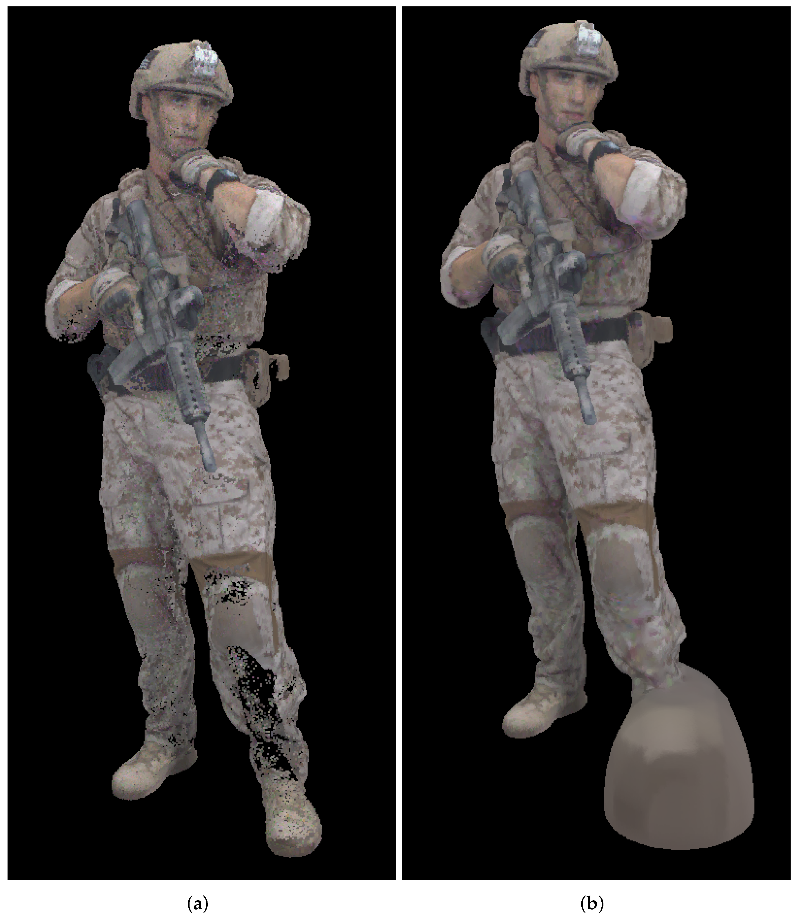
  • normal estimation using CloudCompare version 2.11.1 x64 [46], for the later screened Poisson reconstruction, in “command line” mode. Specific parameters used were: -OCTREE_NORMALS auto -ORIENT PLUS_ZERO -MODEL TRI -ORIENT_NORMS_MST 8 -ORIENT_NORMS_MST 4.
  • Surface Reconstruction: Screened Poisson filter using MeshLab 2020.09 [45]: reconstruction depth 11 and other default values.
  • Poisson-disk Sampling filter using MeshLab: using the same number of samples as the original point cloud, Monte Carlo OverSampling of 20 and other default values. However, usually somewhat higher number of output points were created.
  • Vertex Attribute Transfer filter using MeshLab: using default values.
After the point cloud has been recreated, we need to scale it to its initial size and also translate it to its original position. Those 4 numbers (1 float for scaling and 3 floats for translation in each direction) have to be transmitted as well. Original point cloud snapshot and point cloud snapshots before and after the Poisson reconstruction algorithm are presented in Figure 12.
Tested 20 input point clouds have overall 15,900,190 points, on average 795,010 points per point cloud, while the overall compressed file size is 25.3 × 10 6 B. In this case we use approximately 25.3 × 10 6 × 8 / ( 20 × 795 , 010 ) = 12.7 bits per (input) point, or, if compared with the output number of points, we use approximately 25.3 × 10 6 × 8 / ( 20 × 1 , 154 , 324 ) = 8.8 bits per output point. However, the Poisson reconstruction algorithm at the end of the decompression may produce even higher number of output points (in this case average number of points is 1,154,324), than the input number of points, so in this case the number of bits per output point may be misleading. Because of that, later we report only bits per input point. Poisson reconstruction step is an important part of the proposed algorithm, cf. Figure 12. Used scripts can be found on the web page [49].

5. Results

5.1. Objective Measures Used for Point Cloud Performance Comparison

Recently, several objective measures have been proposed, based on geometry or/and attribute information of the tested point clouds [50]. For geometry, two different groups of measures have been proposed: point-to-point (p2p) and point-to-plane distances (p2pl) [51]. Later in the paper, as point-to-point measures we will use rmsF p 2 p , rmsFPSNR 1 p 2 p and rmsFPSNR 2 p 2 p measures defined as:
rmsF p 2 p = 1 n i = 1 n | | E i , j | | 2 2
rmsFPSNR 1 p 2 p = 10 log 10 MAX _ DIST ( rmsF p 2 p ) 2
rmsFPSNR 2 p 2 p = 10 log 10 3 c 2 ( rmsF p 2 p ) 2 , c = 2 d 1
In Equation (24), E i , j is defined as the difference vector (or point to nearest point vector) between an arbitrary point from the first point cloud and the corresponding nearest point from the second point cloud. The first and second point clouds are firstly original and degraded and then vice versa. Final (symmetric) measure is calculated as the measure with worse (higher rms) score.
In Equation (25) M A X _ D I S T is maximal distance between all pairs of closest points in the first and second point cloud, as defined in [51]. In Equation (26) c is the peak constant value, depending on the point cloud coordinates precision d (e.g., d = 10 for 10-bit depth precision), as used in [19] during the development of the MPEG standard.
Similar to the point-to-point measures, point-to-plane measures are defined as:
rmsF p 2 pl = 1 n i = 1 n ( < E i , j , N j > ) 2
rmsFPSNR 1 p 2 p = 10 log 10 MAX _ DIST ( rmsF p 2 pl ) 2
rmsFPSNR 2 p 2 p = 10 log 10 3 c 2 ( rmsF p 2 pl ) 2 , c = 2 d 1
In Equation (27) E i , j is defined similarly as for the p2p measures. N j is the unit normal vector, calculated for each point in the first point cloud. < E i , j , N j > is the dot product between error vector E i , j and normal vector N j , obtaining projected error vector. In Equation (28) parameter MAX _ DIST is the same as in Equation (25) and in Equation (29) parameters c and d are the same as in the Equation (26).
In the next subsection, point-to-point and point-to-plane measures will be calculated using the software presented in [51].

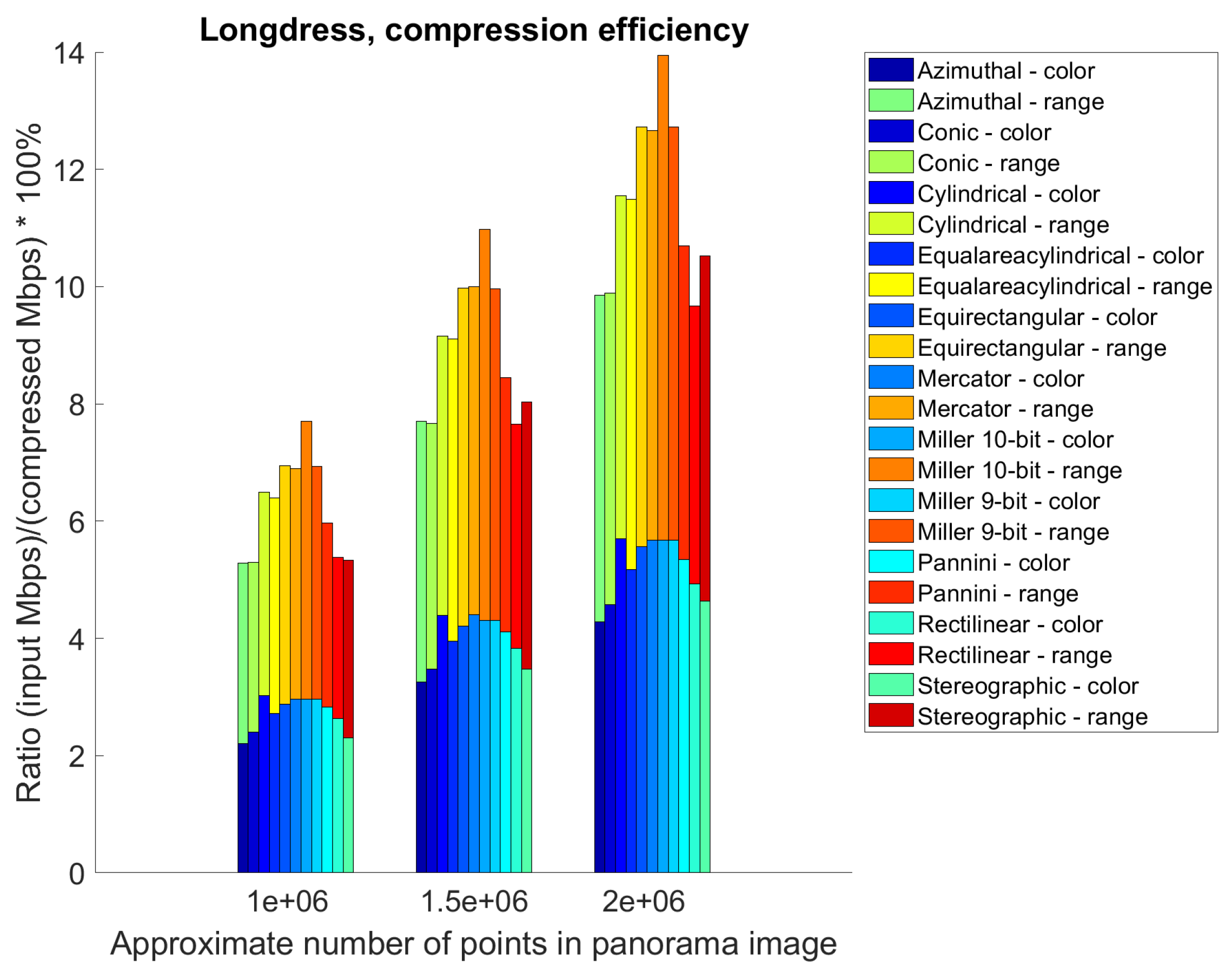
5.2. Point Cloud Compression Using Different Projections—Compression Efficiency

Table 1, Table 2 and Table 3 present a basic overview of the compression efficiency of point clouds with different projection area: 1056 × 944 pixels (approximately 1,000,000), 1296 × 1160 pixels (approximately 1,500,000) and 1496 × 1344 pixels (approximately 2,000,000) respectively. Separately, we calculated bpp (bits per input point) and Mbps (bpp × average number of input points per point cloud × 30 point clouds per second × 10 6 ) for color, range and color+range compressed video files. Results from all three tables are also summarized in the Figure 13, which represents average ratio of the input file sizes and the color and range compressed video file sizes, created from the panorama images, using point cloud Longdress. Higher ratio does not represent better case (i.e., better objective scores), but only higher number of used bits per input point, for the same panorama size. It can be concluded that equirectangular, Miller and Mercator projections have the highest bpp for the tested point cloud Longdress.

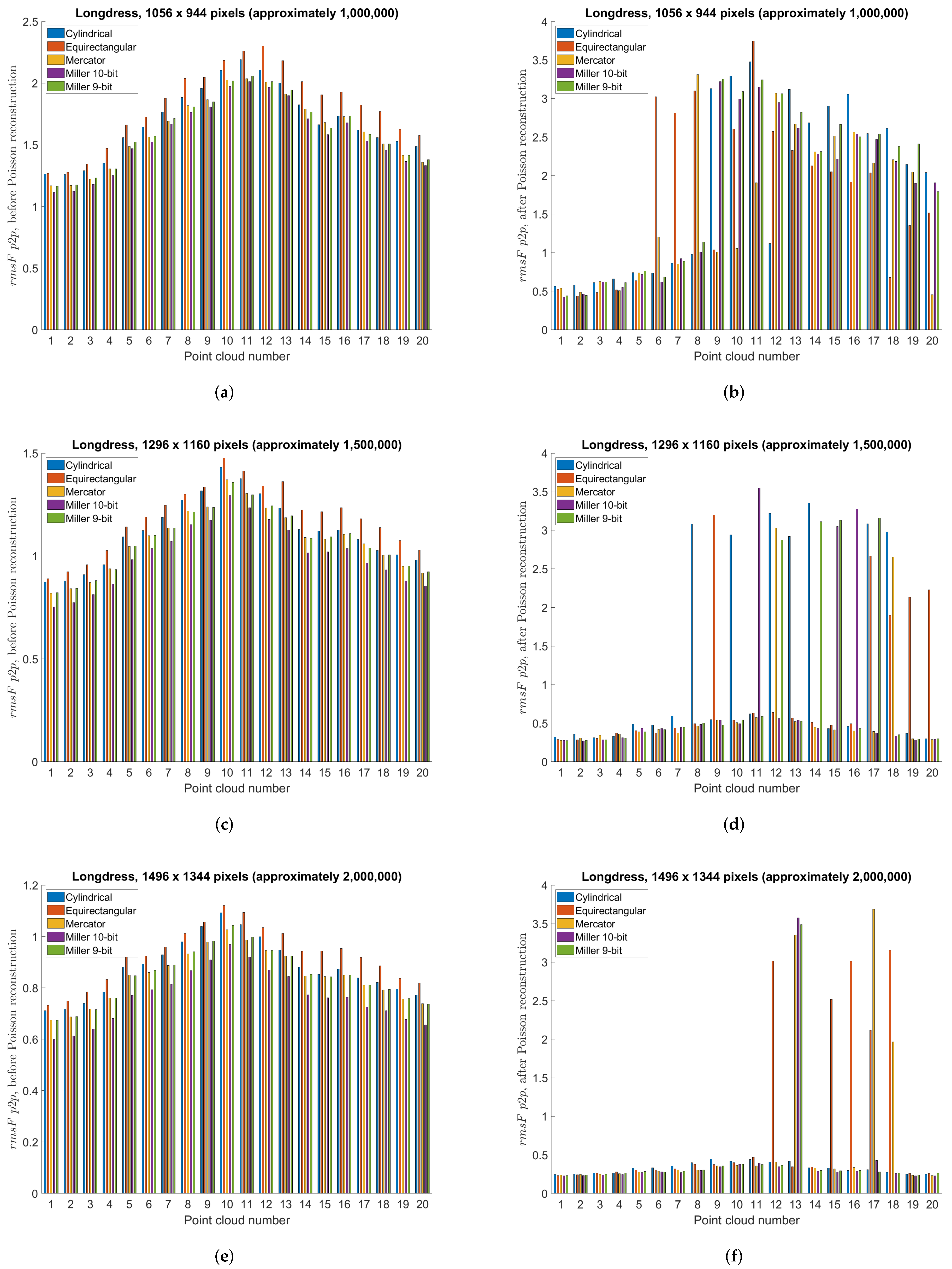
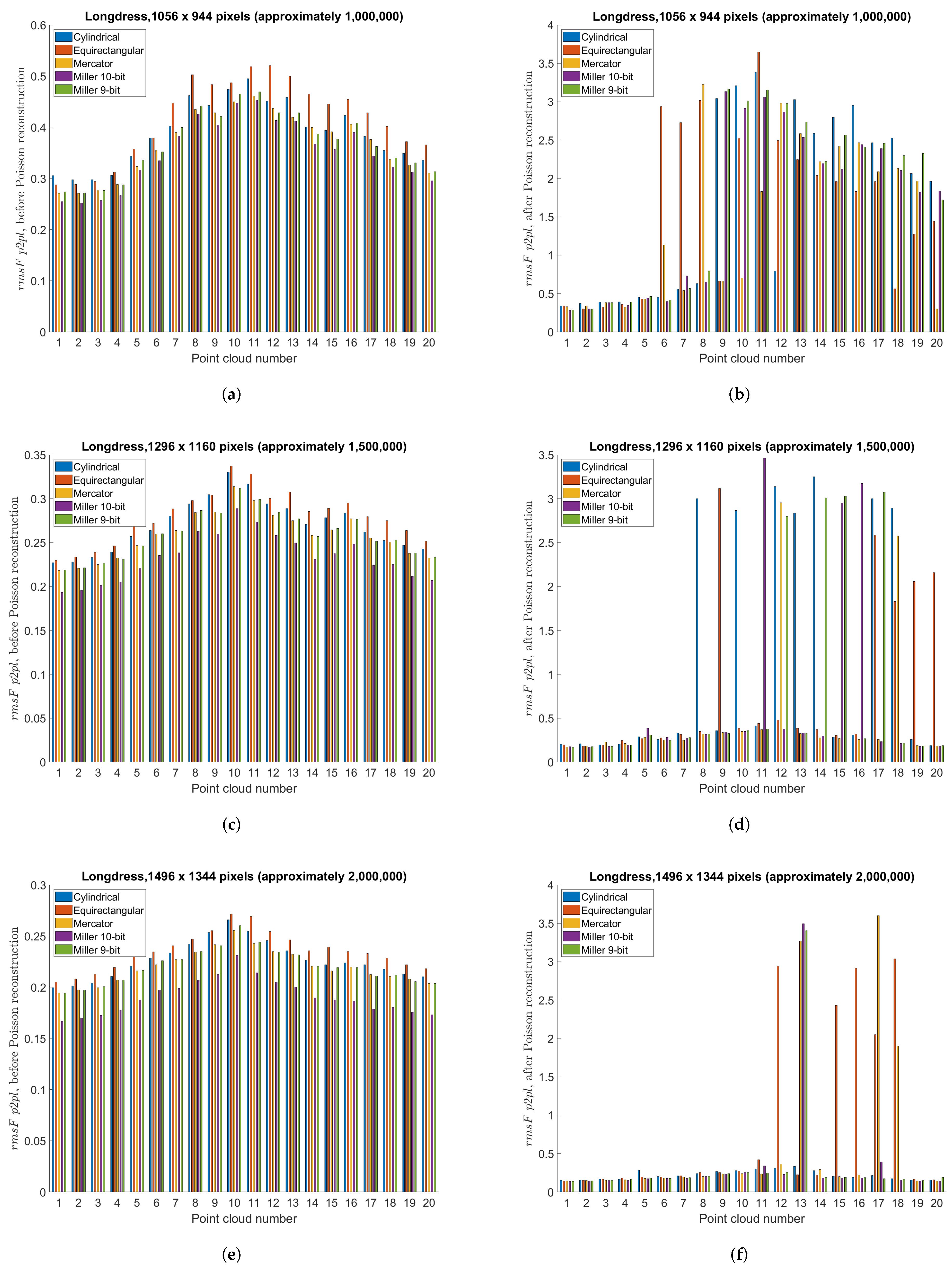
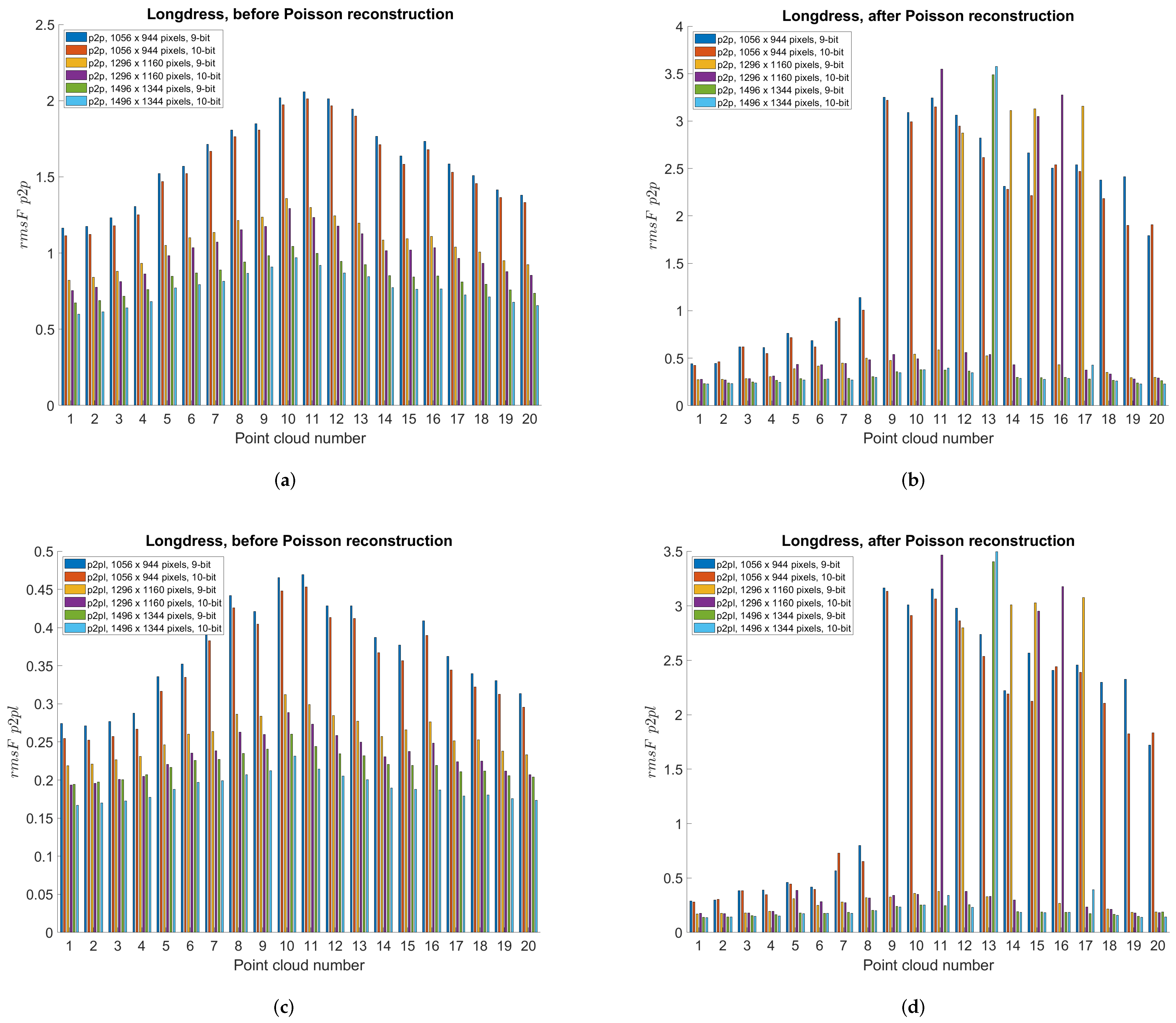
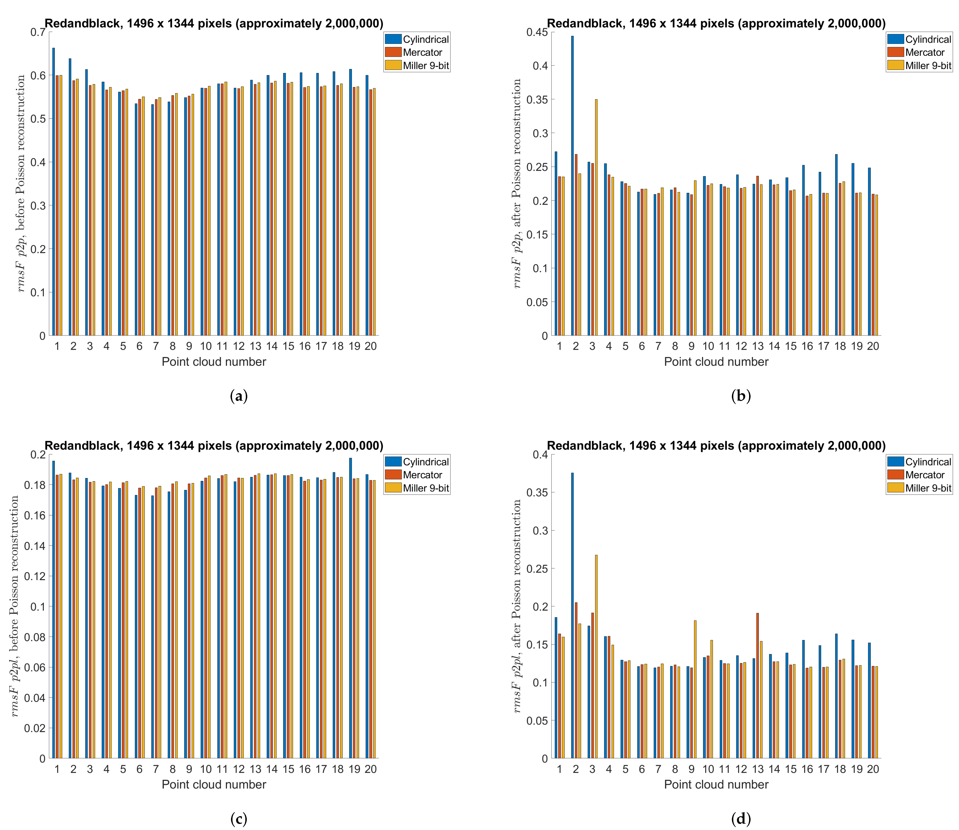
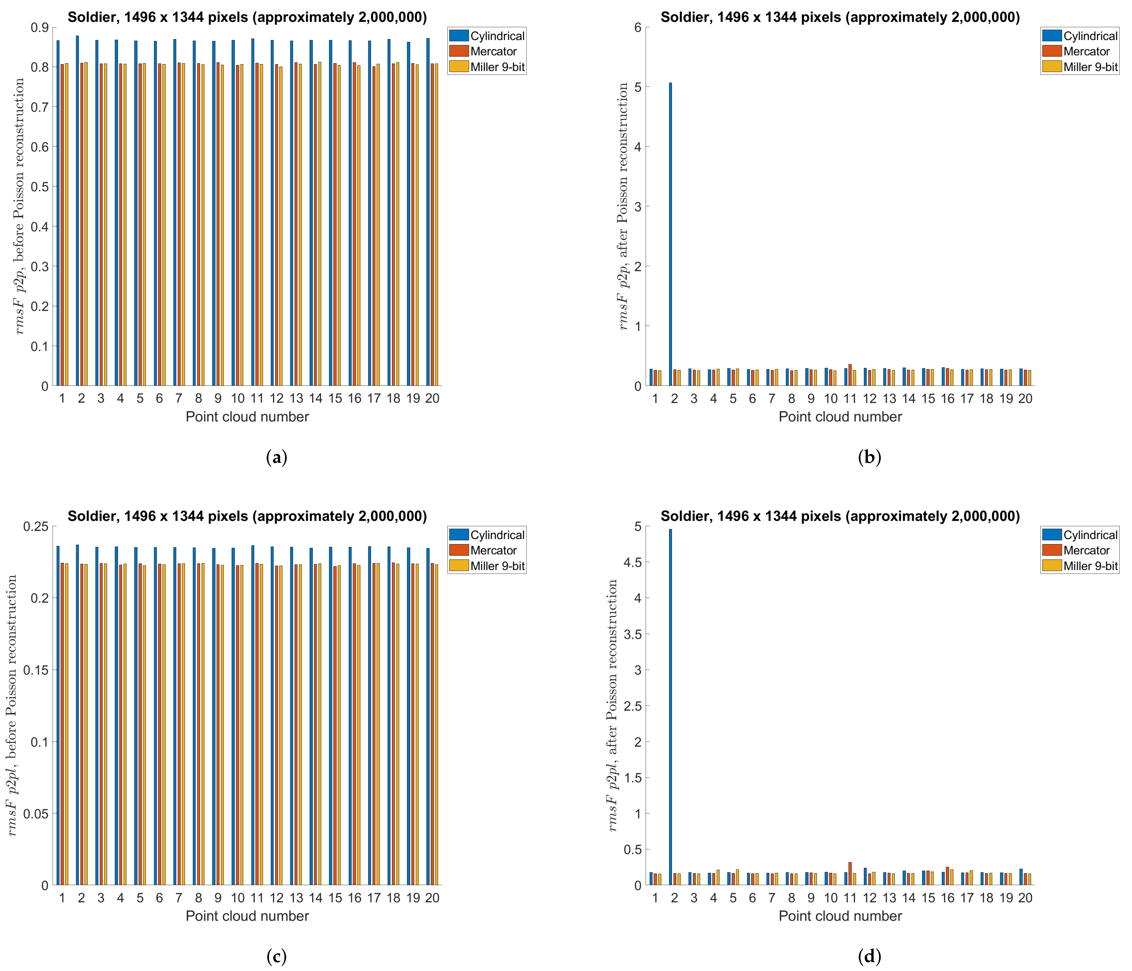
5.3. Point Cloud Compression Using Different Projections—Objective Measures

This section compares different projection methods with three different panorama sizes using previously described point-to-point and point-to-plane objective measures. Specifically, Table 4, Table 5 and Table 6 present objective measures before Poisson reconstruction, while Table 7, Table 8 and Table 9 present objective measures after Poisson reconstruction. Best values are bolded in all tables. Figure 14 presents point-to-point measure separately per each point cloud, for cylindrical, equirectangular, Mercator, Miller 10-bit and Miller 9-bit projections, before and after Poisson reconstruction, for all three panorama sizes, while Figure 15 similarly presents point-to-plane measure. Finally, Figure 16 compares 9-bit and 10-bit Miller projections using point-to-point and point-to-plane measures, before and after Poisson reconstruction.

5.4. Point Cloud Compression—Timing Performance

In this section we will present timing performance for the case of Miller 9-bit projection with panorama size of 2,000,000 points, Table 10. Point cloud to panorama and vice versa timing is averaged across 20 point clouds, while for video compression and decompression we use FFmpeg and different video compressions for geometry and texture images described earlier. For texture, we use the x265 coder (H.265/HEVC) with lossy compression, while for geometry we use the FFV1 coder with lossless compression. For x265 (for texture) we use crf 17 (constant rate factor), pixel format rgb24, preset veryslow, while for FFV1 (for geometry) we use pixel format gray9le (depth of 9 bits per pixel). Computer performance is: Intel i7-4770 @ 3.40 GHz, 16 GB RAM, using virtual machine on Windows 7 x64, running Ubuntu x64 18.04 LTS. It can be seen that Poisson reconstruction and upsampling process takes most of the overall time, compared with other steps. Minor steps in between presented were not taken into account (creating readable point clouds for CloudCompare and Meshlab by adding header in created point clouds from 3DTK and copying files). Due to the overall timing, we did not test all 300 point clouds in a Longdress sequence, but we used first 20 point clouds. However, we expect similar performance for the other point clouds as well.

5.5. Point Cloud Compression Using Different Point Clouds

In this section we will present results for two different dynamic point clouds, Redandblack and Soldier (Figure 17) from the dynamic point cloud dataset [44]. Similar to the previous test cases, we used 20 point clouds from the beginning (“redandblack_vox10_1450.ply”–“redandblack_vox10_1469.ply” and “soldier_vox10_0536.ply” – “soldier_vox10_0555.ply”). Panorama image size of approximately 2,000,000 points and cylindrical, Mercator and Miller 9-bit projection types have been used. Results for the point-to-point and point-to-plane measures are shown in Figure 18 for Redandblack and Figure 19 for Soldier point clouds.
Figure 20 shows second decompressed point cloud Soldier, using cylindrical projection with panorama size of 2,000,000 points, “soldier_vox10_0537.ply”. In Figure 20a we don’t use Poisson reconstruction, while in Figure 20b we use Poisson reconstruction algorithm described earlier. It can be seen that in Figure 20a there are missing points on the left leg, which creates wrongly oriented normals and in Figure 20b there exist an artifact, not present in the original point cloud. Due to this error, there is a noticeable increase (lower quality) of point-to-point and point-to-plane measures, as it can be seen in Figure 19b,d, for the point cloud number 2 and cylindrical projection (blue color).

5.6. Comparison with Octree Reduction from 3DTK Toolkit

In this section we will present results using 3DTK toolkit and octree reduction method, for the previously tested point clouds: Longdress (Table 11 and Table 12), Redandblack (Table 13 and Table 14) and Soldier (Table 15 and Table 16). Generally, parameter “R” turns on octree based point reduction with voxels of size R 3 , while parameter “O” enables randomized octree based point reduction with O points per voxel. We used “scan_red” and “show” programs from 3DTK toolkit to create reduced point clouds: “scan_red” to create decompressed octree-based reduced point clouds and “show” to create compressed .oct files. With increasing “R” we create lower number of points, while with increasing “O” we create higher number of output points. Decompressed point clouds have been compared with the original point clouds using previously described point-to-point and point-to-plane metrics. Average size of output .oct file is also reported, as well as their bits per input point (bpp).

5.7. Discussion

From Table 4, Table 5 and Table 6 e.g., before the Poisson surface reconstruction algorithm, the best projection is Miller 10-bit, however Miller 9-bit and Mercator (also 9-bit) are similarly performed. Probably because of the higher bit depth, Miller 10-bit is here the best projection, however 1 extra bit may not be justified by only a little better objective measures, Figure 16. From Table 7, Table 8 and Table 9 e.g., after the Poisson reconstruction algorithm, Mercator projection is the best in the cases with projection areas of 1056 × 944 pixels and 1296 × 1160 pixels, while cylindrical projection is the best for the projection area of 1496 × 1344 pixels. In the case of the bigger projection area, there are more points, so surface reconstruction algorithm gives better results. Actually, the main problem is the automatic calculation of normal vectors: in some cases, inverted normal vectors are calculated so Poisson reconstruction algorithm afterwards creates unwanted artifacts, lowering the overall objective score rmsF. If the point clouds originate from sensor measurements, then the sensor poses enable a consistent orientation of the normal vectors. Artifacts from inconsistent normals are noticable in Figure 14 and Figure 15 as higher scores in those point clouds. It can be seen that in the best case, e.g., cylindrical projection with a projection area of 1496 × 1344 pixels, Figure 15f, there are no unexpected errors, so the average score is the best for this case. The Miller projection also gives very good results, with only 1 larger error for the largest projection area. However, with smaller projection areas, some of the points in the original point cloud become occluded by other points, so that they are not visible in the used projection. Because of that, larger holes appear in the decompressed point cloud, which makes it difficult to calculate normal vectors and finally surface reconstruction. This can be seen especially in the smallest projection area that was tested, with a size 1056 × 944 pixels. In this case, average rmsF objective score measures are the same before and after surface reconstruction, meaning that the results were not better with the reconstruction algorithm. From Figure 18, Redandblack point cloud, all proposed projections generally give good results with Poisson reconstruction. From Figure 19, Soldier point cloud, Mercator and Miller projections give good results with Poisson reconstruction, while cylindrical projection creates one error for the second point cloud. Possibly, newer projection maps might be used, for example as in the irregularly shaped objects in astronomy [52].
In Equation (22) we are using 16-bit precision, newly added in 3DTK toolkit, so that in this paper we have the best representation for 16-bit precision, which can be also saved in png file and stored using 3DTK toolkit (which uses OpenCV to store images). However, later we are compressing geometry using 9-bit (or 10-bit for Miller compression) and FFV1 video compression. FFV1 decoder also creates 16-bit png images, but with maximally 2 9 (or 2 10 ) different intensities. This is different, compared to the reference [9], because in the reference [9] we used only 24-bit geometry precision, before video compression. Compared with the reference [9], similar parameters were for 1920x1080 resolution and equirectangular projection, where 64,160,627 bytes (for the geometry and color) were used, while in this paper for panorama size of 2,000,000 and equirectangular projection we use 12.7261 bits per point or (multiplied by 795,010 average number of input points and 20 point clouds) 25,293,426 bytes, which is 39.4% from [9]. Separately, in [9] we use 21,378,775 bytes for the geometry, while in this paper we use 14,225,893 bytes or 66.5% from [9]. For the color, in [9] we use 43,208,605 bytes, while in this paper we use 11,067,533 bytes or 25.6% from [9]. Also, somewhat better pixel occupancy is achieved in this paper, compared to the reference [9]: for the same case (and equirectangular projection), average decompressed point cloud Longdress has 428,221 points (before Poisson reconstruction) in this paper and 398,905 in [9]. This might be also compared with equirectangular projection and panorama size of 1,500,000 points, where average decompressed point cloud has 390,058 points (before Poisson reconstruction). For this case, we use 9.9778 bits per point or 19,831,040 bytes. which is 30.9% from [9]. Better projection methods, like Miller, gives for the same panorama size (1,500,000 points) on average higher number of output point cloud points—406,868 and also needs 19,789,828 bytes for the geometry and color, or 30.8% from [9]. In the reference [10], larger static point clouds were also used with bigger range dynamic, which might need 24-bit representation. However, in this paper we used only voxelized dynamic point clouds with the size 1024 × 1024 × 1024 , so 9-bit representation might be enough.
In comparison with the results from octree reduction, the proposed solution gives better results for a similar size. However, the octree reduction algorithm has not been designed for dynamic point clouds, and it was designed for other types of point clouds, such as point clouds created by LIDAR, with non-uniform density and sampling, with much higher bit-depth, in which case results might be different. Also, in octree-based reduction, points do not occlude each other, so it creates a uniformly (sub)sampled point cloud, independent of the final number of points, compared to the proposed solution.

6. Conclusions

In this paper, we have proposed a new projection-based point cloud compression using different projection types, video compression algorithms, and surface reconstruction algorithm. Ten different projection types and three different projection area sizes have been considered, and objective point-to-point and point-to-plane measures were calculated. The results showed that, overall, the Miller projection can be considered as the best among the tested projections. The Mercator projection needs to be modified to address the problem of representing latitudes φ near ± 90 . Cylindrical projection has worse objective scores for smaller panorama size (among tested sizes). Also, although the Poisson surface reconstruction can imply some artifacts due to the missing points in the raw decompressed point cloud, it is an important step of the proposed point cloud compression which fills the missing points and usually generates better visual quality of reconstructed point clouds, at least for larger panorama sizes and tested point clouds.
Future research will consider different projection types which may keep points without creating larger holes and better algorithms for normal vector calculation which may provide higher compression ratios. Different empty-pixel color filling methods might also be considered in future research, such as horizontal filling used by MPEG’s V-PCC compression.

Author Contributions

Conceptualization, E.D.; methodology, E.D. and A.B.; software, E.D. and A.N.; validation, E.D., A.B. and A.N.; formal analysis, E.D.; investigation, E.D. and A.B.; resources, A.N.; data curation, E.D.; writing—original draft preparation, E.D.; writing—review and editing, A.B. and A.N. All authors have read and agreed to the published version of the manuscript.

Funding

This research received no external funding.

Data Availability Statement

The data presented in this study are openly available at http://msl.unin.hr/ accessed on 13 September 2021.

Acknowledgments

This publication was supported by the Open Access Publication Fund of the University of Würzburg.

Conflicts of Interest

The authors declare no conflict of interest.

References

  1. Astola, P.; da Silva Cruz, L.A.; da Silva, E.A.; Ebrahimi, T.; Freitas, P.G.; Gilles, A.; Oh, K.J.; Pagliari, C.; Pereira, F.; Perra, C.; et al. JPEG Pleno: Standardizing a Coding Framework and Tools for Plenoptic Imaging Modalities. ITU J. ICT Discov. 2020, 3, 1–15. [Google Scholar] [CrossRef]
  2. Perkis, A.; Timmerer, C.; Baraković, S.; Husić, J.B.; Bech, S.; Bosse, S.; Botev, J.; Brunnström, K.; Cruz, L.; Moor, K.D.; et al. QUALINET White Paper on Definitions of Immersive Media Experience (IMEx). In Proceedings of the European Network on Quality of Experience in Multimedia Systems and Services, 14th QUALINET Meeting, Online, 25 May 2020; pp. 1–15. [Google Scholar]
  3. Wang, Q.; Tan, Y.; Mei, Z. Computational Methods of Acquisition and Processing of 3D Point Cloud Data for Construction Applications. Arch. Comput. Methods Eng. 2020, 27, 479–499. [Google Scholar] [CrossRef]
  4. Pereira, F.; da Silva, E.A.; Lafruit, G. Chapter 2—Plenoptic imaging: Representation and processing. In Academic Press Library in Signal Processing; Chellappa, R., Theodoridis, S., Eds.; Elsevier: Amsterdam, The Netherlands, 2018; Volume 6, pp. 75–111. [Google Scholar] [CrossRef]
  5. van der Hooft, J.; Vega, M.T.; Timmerer, C.; Begen, A.C.; De Turck, F.; Schatz, R. Objective and Subjective QoE Evaluation for Adaptive Point Cloud Streaming. In Proceedings of the 2020 Twelfth International Conference on Quality of Multimedia Experience (QoMEX), Athlone, Ireland, 26–28 May 2020; pp. 1–6. [Google Scholar] [CrossRef]
  6. Han, B.; Liu, Y.; Qian, F. ViVo: Visibility-aware mobile volumetric video streaming. In Proceedings of the 26th Annual International Conference on Mobile Computing and Networking, MobiCom 2020, London, UK, 21–25 September 2020; pp. 137–149. [Google Scholar] [CrossRef]
  7. Dumic, E.; Battisti, F.; Carli, M.; da Silva Cruz, L.A. Point Cloud Visualization Methods: A Study on Subjective Preferences. In Proceedings of the 2020 28th European Signal Processing Conference (EUSIPCO), Amsterdam, The Netherlands, 18–21 January 2020; pp. 1–5. [Google Scholar]
  8. Javaheri, A.; Brites, C.; Pereira, F.M.B.; Ascenso, J.M. Point Cloud Rendering after Coding: Impacts on Subjective and Objective Quality. IEEE Trans. Multimed. 2020, 23, 4049–4064. [Google Scholar] [CrossRef]
  9. Dumic, E.; Bjelopera, A.; Nüchter, A. Projection based dynamic point cloud compression using 3DTK toolkit and H.265/HEVC. In Proceedings of the 2019 2nd International Colloquium on Smart Grid Metrology (SMAGRIMET), Split, Croatia, 9–12 April 2019; pp. 1–4. [Google Scholar] [CrossRef]
  10. da Silva Cruz, L.A.; Dumić, E.; Alexiou, E.; Prazeres, J.; Duarte, R.; Pereira, M.; Pinheiro, A.; Ebrahimi, T. Point cloud quality evaluation: Towards a definition for test conditions. In Proceedings of the 2019 Eleventh International Conference on Quality of Multimedia Experience (QoMEX), Berlin, Germany, 5–7 June 2019; pp. 1–6. [Google Scholar] [CrossRef] [Green Version]
  11. Elseberg, J.; Borrmann, D.; Nüchter, A. One billion points in the cloud—An octree for efficient processing of 3D laser scans. ISPRS J. Photogramm. Remote Sens. 2013, 76, 76–88. [Google Scholar] [CrossRef]
  12. Elseberg, J.; Magnenat, S.; Siegwart, R.; Nüchter, A. Comparison of nearest-neighbor-search strategies and implementations for efficient shape registration. J. Softw. Eng. Robot. 2013, 3, 2–12. [Google Scholar] [CrossRef]
  13. 3DTK—The 3D Toolkit. Available online: http://slam6d.sourceforge.net/ (accessed on 13 September 2021).
  14. Houshiar, H.; Borrmann, D.; Elseberg, J.; Nüchter, A. Panorama based point cloud reduction and registration. In Proceedings of the 2013 16th International Conference on Advanced Robotics (ICAR), Montevideo, Uruguay, 25–29 November 2013; pp. 1–8. [Google Scholar] [CrossRef]
  15. Houshiar, H.; Nüchter, A. 3D point cloud compression using conventional image compression for efficient data transmission. In Proceedings of the 2015 XXV International Conference on Information, Communication and Automation Technologies (ICAT), Sarajevo, Bosnia and Herzegovina, 29–31 October 2015; pp. 1–8. [Google Scholar] [CrossRef]
  16. Mammou, K.; Chou, P.A.; Flynn, D.; Krivokuća, M.; Nakagami, O.; Sugio, T. G-PCC Codec Description v2; Technical Report, ISO/IEC JTC1/SC29/WG11 Input Document N18189; MPEG: Marrakech, MA, USA, 2019. [Google Scholar]
  17. Zakharchenko, V. V-PCC Codec Description; Technical Report, ISO/IEC JTC1/SC29/WG11 Input Document N18190; MPEG: Marrakech, MA, USA, 2019. [Google Scholar]
  18. Sullivan, G.J.; Ohm, J.; Han, W.; Wiegand, T. Overview of the High Efficiency Video Coding (HEVC) Standard. IEEE Trans. Circuits Syst. Video Technol. 2012, 22, 1649–1668. [Google Scholar] [CrossRef]
  19. Schwarz, S.; Preda, M.; Baroncini, V.; Budagavi, M.; Cesar, P.; Chou, P.A.; Cohen, R.A.; Krivokuća, M.; Lasserre, S.; Li, Z.; et al. Emerging MPEG Standards for Point Cloud Compression. IEEE J. Emerg. Sel. Top. Circuits Syst. 2019, 9, 133–148. [Google Scholar] [CrossRef] [Green Version]
  20. Graziosi, D.; Nakagami, O.; Kuma, S.; Zaghetto, A.; Suzuki, T.; Tabatabai, A. An overview of ongoing point cloud compression standardization activities: Video-based (V-PCC) and geometry-based (G-PCC). APSIPA Trans. Signal Inf. Process. 2020, 9, e13. [Google Scholar] [CrossRef] [Green Version]
  21. Alexiou, E.; Viola, I.; Borges, T.M.; Fonseca, T.A.; de Queiroz, R.L.; Ebrahimi, T. A comprehensive study of the rate-distortion performance in MPEG point cloud compression. APSIPA Trans. Signal Inf. Process. 2019, 8, 27. Available online: https://www.epfl.ch/labs/mmspg/quality-assessment-for-point-cloud-compression/ (accessed on 13 September 2021). [CrossRef] [Green Version]
  22. Perry, S.; Cong, H.P.; da Silva Cruz, L.A.; Prazeres, J.; Pereira, M.; Pinheiro, A.; Dumic, E.; Alexiou, E.; Ebrahimi, T. Quality Evaluation of Static Point Clouds Encoded Using MPEG Codecs. In Proceedings of the 2020 IEEE International Conference on Image Processing (ICIP), Abu Dhabi, United Arab Emirates, 25–28 October 2020; pp. 3428–3432. [Google Scholar] [CrossRef]
  23. Alexiou, E.; Tung, K.; Ebrahimi, T. Towards neural network approaches for point cloud compression. In Proceedings Volume 11510, Applications of Digital Image Processing XLIII; International Society for Optics and Photonics: Bellingham, WA, USA, 2020; p. 1151008. [Google Scholar] [CrossRef]
  24. Mekuria, R.; Blom, K.; Cesar, P. Design, Implementation, and Evaluation of a Point Cloud Codec for Tele-Immersive Video. IEEE Trans. Circuits Syst. Video Technol. 2017, 27, 828–842. [Google Scholar] [CrossRef] [Green Version]
  25. Quach, M.; Valenzise, G.; Dufaux, F. Learning Convolutional Transforms for Lossy Point Cloud Geometry Compression. In Proceedings of the 2019 IEEE International Conference on Image Processing, ICIP 2019, Taipei, Taiwan, 22–25 September 2019; pp. 4320–4324. [Google Scholar] [CrossRef] [Green Version]
  26. Loop, C.; Cai, Q.; Escolano, S.O.; Chou, P. Microsoft Voxelized Upper Bodies—A Voxelized Point Cloud Dataset; Technical Report, ISO/IEC JTC1/SC29 Joint WG11/WG1 (MPEG/JPEG) Input Document m38673/M72012. 2016. Available online: http://plenodb.jpeg.org/pc/microsoft/ (accessed on 13 September 2021).
  27. Quach, M.; Valenzise, G.; Dufaux, F. Improved Deep Point Cloud Geometry Compression. In Proceedings of the 2020 IEEE 22nd International Workshop on Multimedia Signal Processing (MMSP), Tampere, Finland, 21–24 September 2020; pp. 1–6. [Google Scholar] [CrossRef]
  28. Wang, J.; Zhu, H.; Liu, H.; Ma, Z. Lossy Point Cloud Geometry Compression via End-to-End Learning. IEEE Trans. Circuits Syst. Video Technol. 2021, 31, 4909–4923. [Google Scholar] [CrossRef]
  29. Wang, J.; Ding, D.; Li, Z.; Ma, Z. Multiscale Point Cloud Geometry Compression. In Proceedings of the 2021 Data Compression Conference (DCC), Virtual, 23–26 March 2021; pp. 73–82. [Google Scholar] [CrossRef]
  30. Guarda, A.F.R.; Rodrigues, N.M.M.; Pereira, F. Point Cloud Coding: Adopting a Deep Learning-based Approach. In Proceedings of the 2019 Picture Coding Symposium (PCS), Ningbo, China, 12–15 November 2019; pp. 1–5. [Google Scholar] [CrossRef]
  31. Rusu, R.B.; Cousins, S. 3D is here: Point Cloud Library (PCL). In Proceedings of the IEEE International Conference on Robotics and Automation (ICRA), Shanghai, China, 9–13 May 2011. [Google Scholar]
  32. Guarda, A.F.R.; Rodrigues, N.M.M.; Pereira, F. Deep Learning-based Point Cloud Geometry Coding with Resolution Scalability. In Proceedings of the 2020 IEEE 22nd International Workshop on Multimedia Signal Processing (MMSP), Tampere, Finland, 21–24 September 2020; pp. 1–6. [Google Scholar] [CrossRef]
  33. Guarda, A.F.R.; Rodrigues, N.M.M.; Pereira, F. Adaptive Deep Learning-Based Point Cloud Geometry Coding. IEEE J. Sel. Top. Signal Process. 2021, 15, 415–430. [Google Scholar] [CrossRef]
  34. Milani, S. ADAE: Adversarial Distributed Source Autoencoder For Point Cloud Compression. In Proceedings of the 2021 IEEE International Conference on Image Processing (ICIP), Anchorage, AK, USA, 19–22 September 2021; pp. 3078–3082. [Google Scholar] [CrossRef]
  35. Lazzarotto, D.; Alexiou, E.; Ebrahimi, T. On Block Prediction For Learning-Based Point Cloud Compression. In Proceedings of the 2021 IEEE International Conference on Image Processing (ICIP), Anchorage, AK, USA, 19–22 September 2021; pp. 3378–3382. [Google Scholar] [CrossRef]
  36. Yan, W.; Shao, Y.; Liu, S.; Li, T.H.; Li, Z.; Li, G. Deep AutoEncoder-based Lossy Geometry Compression for Point Clouds. arXiv 2019, arXiv:1905.03691. Available online: https://arxiv.org/abs/1905.03691 (accessed on 13 September 2021).
  37. Huang, T.; Liu, Y. 3D Point Cloud Geometry Compression on Deep Learning. In Proceedings of the 27th ACM International Conference on Multimedia, Nice, France, 21–25 October 2019; Association for Computing Machinery: New York, NY, USA, 2019; pp. 890–898. [Google Scholar] [CrossRef]
  38. Nguyen, D.T.; Quach, M.; Valenzise, G.; Duhamel, P. Learning-Based Lossless Compression of 3D Point Cloud Geometry. In Proceedings of the ICASSP 2021–2021 IEEE International Conference on Acoustics, Speech and Signal Processing (ICASSP), Toronto, ON, Canada, 6–11 June 2021; pp. 4220–4224. [Google Scholar] [CrossRef]
  39. Nguyen, D.T.; Quach, M.; Valenzise, G.; Duhamel, P. Multiscale deep context modeling for lossless point cloud geometry compression. In Proceedings of the 2021 IEEE International Conference on Multimedia & Expo Workshops (ICMEW), Shenzhen, China, 5–9 July 2021. [Google Scholar] [CrossRef]
  40. Que, Z.; Lu, G.; Xu, D. VoxelContext-Net: An Octree based Framework for Point Cloud Compression. In Proceedings of the IEEE/CVF Conference on Computer Vision and Pattern Recognition, CVPR 2021, Virtual, 19–25 June 2021; pp. 6042–6051. [Google Scholar]
  41. Lazzarotto, D.; Ebrahimi, T. Learning residual coding for point clouds. In Applications of Digital Image Processing XLIV; Tescher, A.G., Ebrahimi, T., Eds.; International Society for Optics and Photonics: Washington, DC, USA, 2021; Volume 11842, pp. 223–235. [Google Scholar] [CrossRef]
  42. Weisstein, E.W. Map Projection. From MathWorld—A Wolfram Web Resource. Available online: https://mathworld.wolfram.com/topics/MapProjections.html (accessed on 16 April 2021).
  43. Houshiar, H. Documentation and Mapping with 3D Point Cloud Processing. Ph.D. Thesis, University of Würzburg, Würzburg, Germany, 2017. [Google Scholar] [CrossRef]
  44. d’Eon, E.; Harrison, B.; Myers, T.; Chou, P.A. 8i Voxelized Full Bodies—A Voxelized Point Cloud Dataset; Technical Report, ISO/IEC JTC1/SC29 Joint WG11/WG1 (MPEG/JPEG) Input Document WG11M40059/WG1M74006. 2017. Available online: https://jpeg.org/plenodb/pc/8ilabs/ (accessed on 13 September 2021).
  45. Lab, Visual Computing, MeshLab. Available online: http://www.meshlab.net/ (accessed on 13 September 2021).
  46. CloudCompare—3D Point Cloud and Mesh Processing Software—Open Source Project. Available online: http://www.cloudcompare.org (accessed on 6 February 2019).
  47. FFmpeg Team. FFmpeg. Available online: https://www.ffmpeg.org/download.html (accessed on 2 May 2021).
  48. Weisstein, E.W. Voronoi Diagram. From MathWorld—A Wolfram Web Resource. Available online: https://mathworld.wolfram.com/VoronoiDiagram.html (accessed on 6 November 2021).
  49. Dumic, E. Scripts for Dynamic Point Cloud Compression. Available online: http://msl.unin.hr/ (accessed on 8 November 2021).
  50. Dumic, E.; da Silva Cruz, L.A. Point Cloud Coding Solutions, Subjective Assessment and Objective Measures: A Case Study. Symmetry 2020, 12, 1955. [Google Scholar] [CrossRef]
  51. Tian, D.; Ochimizu, H.; Feng, C.; Cohen, R.; Vetro, A. Geometric distortion metrics for point cloud compression. In Proceedings of the 2017 IEEE International Conference on Image Processing (ICIP), Beijing, China, 17–20 September 2017; pp. 3460–3464. [Google Scholar] [CrossRef]
  52. Grieger, B. Quincuncial adaptive closed Kohonen (QuACK) map for the irregularly shaped comet 67P/Churyumov-Gerasimenko. Astron. Astrophys. 2019, 630, A1. [Google Scholar] [CrossRef] [Green Version]
Figure 1. Panorama images created using point cloud “longdress_vox10_1060.ply” from the Lambert azimuthal equal-area projection, for the geometry (a) and texture (b).
Sensors 22 00197 g001
Figure 2. Panorama images created using point cloud “longdress_vox10_1060.ply” from the Albers equal-area conic projection, for the geometry (a) and texture (b).
Sensors 22 00197 g002
Figure 3. Panorama images created using point cloud “longdress_vox10_1060.ply” from the cylindrical projection, for the geometry (a) and texture (b).
Sensors 22 00197 g003
Figure 4. Panorama images created using point cloud “longdress_vox10_1060.ply” from the cylindrical equal-area projection, for the geometry (a) and texture (b).
Sensors 22 00197 g004
Figure 5. Panorama images created using point cloud “longdress_vox10_1060.ply” from the equirectangular projection, for the geometry (a) and texture (b).
Sensors 22 00197 g005
Figure 6. Panorama images created using point cloud “longdress_vox10_1060.ply” from the Mercator projection, for the geometry (a) and texture (b).
Sensors 22 00197 g006
Figure 7. Panorama images created using point cloud “longdress_vox10_1060.ply” from the Miller projection, for the geometry (a) and texture (b).
Sensors 22 00197 g007
Figure 8. Panorama images created using point cloud “longdress_vox10_1060.ply” from the rectilinear projection, for the geometry (a) and texture (b).
Sensors 22 00197 g008
Figure 9. Panorama images created using point cloud “longdress_vox10_1060.ply” from the Pannini projection, for the geometry (a) and texture (b).
Sensors 22 00197 g009
Figure 10. Panorama images created using point cloud “longdress_vox10_1060.ply” from the stereographic projection, for the geometry (a) and texture (b).
Sensors 22 00197 g010
Figure 11. Point clouds to panorama, using Miller projection: (a) original point cloud “longdress_vox10_1060.ply” (799,765 points); (b) geometry (1496 × 1344 pixels, 16-bit grayscale); (c) texture (1496 × 1344 pixels, 24-bit RGB); (d) texture with Voronoi (1496 × 1344 pixels, 24-bit RGB).
Sensors 22 00197 g011
Figure 12. Point clouds to panorama, using Miller projection and 9-bit range depth: (a) Original point cloud “longdress_vox10_1060.ply” (799,765 points; point size 1 in MeshLab); (b) Decompressed point cloud after Poisson reconstruction (1,161,124 points; point size 1 in MeshLab); (c) Decompressed point cloud before Poisson reconstruction (430,793 points; point size 1 in MeshLab); (d) Decompressed point cloud before Poisson reconstruction (430,793 points; point size 2 in MeshLab).
Sensors 22 00197 g012
Figure 13. Average ratio of the input file sizes and the color and range compressed video file sizes, created from the panorama images, using point cloud Longdress. Ratio is presented for all cases, e.g., for 1,000,000, 1,500,000 and 2,000,000 points.
Sensors 22 00197 g013
Figure 14. Point-to-point objective measure per point cloud, using cylindrical, equirectangular, Mercator, Miller 10-bit and Miller 9-bit projections: (a) before Poisson reconstruction, projection area 1056 × 944 pixels (approximately 1,000,000); (b) after Poisson reconstruction, projection area 1056 × 944 pixels (approximately 1,000,000); (c) before Poisson reconstruction, projection area 1296 × 1160 pixels (approximately 1,500,000); (d) after Poisson reconstruction, projection area 1296 × 1160 pixels (approximately 1,500,000); (e) before Poisson reconstruction, projection area 1496 × 1344 pixels (approximately 2,000,000); (f) after Poisson reconstruction, projection area 1496 × 1344 pixels (approximately 2,000,000).
Sensors 22 00197 g014
Figure 15. Point-to-plane objective measure per point cloud, using cylindrical, equirectangular, Mercator, Miller 10-bit and Miller 9-bit projections: (a) before Poisson reconstruction, projection area 1056 × 944 pixels (approximately 1,000,000); (b) after Poisson reconstruction, projection area 1056 × 944 pixels (approximately 1,000,000); (c) before Poisson reconstruction, projection area 1296 × 1160 pixels (approximately 1,500,000); (d) after Poisson reconstruction, projection area 1296 × 1160 pixels (approximately 1,500,000); (e) before Poisson reconstruction, projection area 1496 × 1344 pixels (approximately 2,000,000); (f) after Poisson reconstruction, projection area 1496 × 1344 pixels (approximately 2,000,000).
Sensors 22 00197 g015
Figure 16. Objective measure per point cloud, using Miller projection with 9-bit depth and 10-bit depth: (a) before Poisson reconstruction, point-to-point measure; (b) after Poisson reconstruction, point-to-point measure; (c) before Poisson reconstruction, point-to-plane measure; (d) after Poisson reconstruction, point-to-plane measure.
Sensors 22 00197 g016
Figure 17. Tested point clouds: (a) Redandblack, “redandblack_vox10_1450.ply”; (b) Soldier, “soldier_vox10_0536.ply”.
Sensors 22 00197 g017
Figure 18. Point-to-point and point-to-plane objective measure ( rmsF p 2 p ) per Redandblack point cloud, using cylindrical, Mercator and Miller 9-bit depth projections with approximately 2,000,000 points: (a) point-to-point, before Poisson reconstruction; (b) point-to-point, after Poisson reconstruction; (c) point-to-plane, before Poisson reconstruction; (d) point-to-plane, after Poisson reconstruction.
Sensors 22 00197 g018
Figure 19. Point-to-point objective measure ( rmsF p 2 p ) per Soldier point cloud, using cylindrical, Mercator and Miller 9-bit depth projections with approximately 2,000,000 points: (a) point-to-point, before Poisson reconstruction; (b) point-to-point, after Poisson reconstruction; (c) point-to-plane, before Poisson reconstruction; (d) point-to-plane, after Poisson reconstruction.
Sensors 22 00197 g019
Figure 20. Decompressed point cloud Soldier, “soldier_vox10_0537.ply”-second point cloud used in compression/decompression process, using cylindrical projection with panorama size of 2,000,000 points: (a) before Poisson reconstruction (point size 2 in MeshLab); (b) after Poisson reconstruction (point size 1 in MeshLab).
Sensors 22 00197 g020
Table 1. Information about the compressed file sizes for different projection types, with projection area of 1056 × 944 pixels (approximately 1,000,000).
1056 × 944 Pixels (Approximately 1,000,000)AzimuthalConicCylindricalEqualareacylindricalEquirectangularMercatorMiller 10-BitMiller 9-BitPanniniRectilinearStereographic
Compressed color average bits per input point (bpp):2.20182.40253.02072.72032.87262.96122.96182.96182.8262.632.3026
Compressed range average bits per input point (bpp):3.07842.89923.47013.67854.0743.93064.73623.96523.13822.75613.0313
Compressed range+color average bits per input point (bpp):5.28035.30166.49086.39876.94676.89187.6986.9275.96425.3865.3339
Input average bits per input point (binary format) (bpp):120.0017120.0017120.0017120.0017120.0017120.0017120.0017120.0017120.0017120.0017120.0017
Ratio (input bpp)/(compressed bpp) * 100%4.40014.4185.4095.33225.78885.74316.41495.77244.97014.48834.4448
Compressed video color (Mbps):52.51457.299372.044964.879268.513570.62670.638770.638767.399962.725754.9167
Compressed video range (Mbps):73.421769.14682.763887.732597.166793.7467112.960894.571374.847565.733172.2982
Compressed video range+color (Mbps):125.9357126.4452154.8087152.6117165.6802164.3727183.5995165.2101142.2474128.4588127.2149
Input point cloud (binary format) (Mbps):2862.07742862.07742862.07742862.07742862.07742862.07742862.07742862.07742862.07742862.07742862.0774
Ratio (input Mbps)/(compressed Mbps) * 100%4.40014.41805.40905.33225.78885.74316.41495.77244.97014.48834.4448
Table 2. Information about the compressed file sizes for different projection types, with projection area of 1296 × 1160 pixels (approximately 1,500,000).
1296 × 1160 Pixels (Approximately 1,500,000)AzimuthalConicCylindricalEqualareacylindricalEquirectangularMercatorMiller 10-BitMiller 9-BitPanniniRectilinearStereographic
Compressed color average bits per input point (bpp):3.25343.47124.39753.94884.20324.40464.30854.30854.11353.83063.4746
Compressed range average bits per input point (bpp):4.44314.19574.75335.15345.77465.59726.67085.64854.32883.81734.5586
Compressed range+color average bits per input point (bpp):7.69657.66699.15089.10229.977810.001810.97939.9578.44237.64798.0332
Input average bits per input point (binary format) (bpp):120.0017120.0017120.0017120.0017120.0017120.0017120.0017120.0017120.0017120.0017120.0017
Ratio (input bpp)/(compressed bpp) * 100%6.41366.3897.62557.5858.31478.33479.14938.29747.03526.37326.6942
Compressed video color (Mbps):77.594982.7901104.88194.18100.2465105.0509102.7599102.759998.10991.3682.8696
Compressed video range (Mbps):105.9685100.0686113.3672122.9091137.726133.4953159.1008134.7181103.243591.0447108.7247
Compressed video range+color (Mbps):183.5634182.8587218.2482217.0891237.9725238.5462261.8607237.4779201.3525182.4047191.5943
Input point cloud (binary format) (Mbps):2862.07742862.07742862.07742862.07742862.07742862.07742862.07742862.07742862.07742862.07742862.0774
Ratio (input Mbps)/(compressed Mbps) * 100%6.41366.38907.62557.58508.31478.33479.14938.29747.03526.37326.6942
Table 3. Information about the compressed file sizes for different projection types, with projection area of 1496 × 1344 pixels (approximately 2,000,000).
1496 ×1344 Pixels (Approximately 2,000,000)AzimuthalConicCylindricalEqualareacylindricalEquirectangularMercatorMiller 10-BitMiller 9-BitPanniniRectilinearStereographic
Compressed color average bits per input point (bpp):4.27584.58045.69755.17325.56855.6755.6695.6695.34344.92984.6411
Compressed range average bits per input point (bpp):5.58115.31185.85446.31417.15766.99088.27187.05435.3484.74285.8841
Compressed range+color average bits per input point (bpp):9.85699.892211.551911.487312.726112.665713.940912.723310.69139.672610.5252
Input average bits per input point (binary format) (bpp):120.0017120.0017120.0017120.0017120.0017120.0017120.0017120.0017120.0017120.0017120.0017
Ratio (input bpp)/(compressed bpp) * 100%8.21398.24349.62659.572610.604910.554611.617210.60268.90938.06048.7709
Compressed video color (Mbps):101.9793109.2427135.8868123.3824132.8104135.3498135.2079135.2079127.4406117.5775110.6906
Compressed video range (Mbps):133.1103126.6887139.6304150.594170.7107166.7318197.286168.2461127.5504113.1165140.3382
Compressed video range+color (Mbps):235.0896235.9314275.5172273.9764303.5211302.0816332.4939303.454254.991230.6941251.0288
Input point cloud (binary format) (Mbps):2862.07742862.07742862.07742862.07742862.07742862.07742862.07742862.07742862.07742862.07742862.0774
Ratio (input Mbps)/(compressed Mbps) * 100%8.21398.24349.62659.572610.604910.554611.617210.60268.90938.06048.7709
Table 4. Point-to-point (p2p) and point-to-plane (p2pl) objective measures rmsF , rmsFPSNR 1 and rmsFPSNR 2 , before Poisson reconstruction, using different projections with projection area of 1056 × 944 pixels (approximately 1,000,000), best values are bold; average input and output number of points and their ratio.
rmsF p 2 p rmsFPSNR 1 p 2 p rmsFPSNR 2 p 2 p rmsF p 2 pl rmsFPSNR 1 p 2 pl rmsFPSNR 2 p 2 pl Average Input PointsAverage Output PointsOutput/Input · 100 %
Azimuthal4.356958.5848−5.78811.137464.42485.8920795,010260,52232.7697
Conic3.848959.1248−4.70801.004864.97786.9979795,010250,45431.5033
Cylindrical1.690162.75062.54350.387869.137815.3180795,010318,70340.0879
Equalareacylindrical3.229059.8909−3.17580.781966.08749.2171795,010283,73735.6897
Equirectangular1.813962.45011.94260.415668.862814.7679795,010333,86541.9951
Mercator1.617762.94592.93420.367769.377715.7978795,010344,68243.3557
Miller 10-bit1.570463.07963.20170.350569.596216.2347795,010345,22343.4237
Miller 9-bit1.620062.93882.92000.368669.368215.7787795,010345,22343.4237
Pannini1.774162.53772.11770.409268.903114.8485795,010291,89036.7153
Rectilinear1.942362.14271.32780.465568.355913.7542795,010260,36832.7503
Stereographic3.626159.3823−4.19300.813565.91168.8655795,010283,55135.6663
Table 5. Point-to-point (p2p) and point-to-plane (p2pl) objective measures rmsF , rmsFPSNR 1 and rmsFPSNR 2 , before Poisson reconstruction, using different projections with projection area of 1296 × 1160 pixels (approximately 1,500,000), best values are bold; average input and output number of points and their ratio.
rmsF p 2 p rmsFPSNR 1 p 2 p rmsFPSNR 2 p 2 p rmsF p 2 pl rmsFPSNR 1 p 2 pl rmsFPSNR 2 p 2 pl Average Input PointsAverage Output PointsOutput/Input · 100 %
Azimuthal3.428159.6300−3.69760.820965.86518.7725795,010313,37239.4174
Conic3.014660.1911−2.57540.779366.09179.2258795,010300,30937.7742
Cylindrical1.121264.51586.07400.269770.684518.4113795,010389,68149.0159
Equalareacylindrical2.425761.1371−0.68350.580867.373511.7893795,010329,72141.4738
Equirectangular1.185164.27225.58680.279770.525118.0925795,010390,05849.0633
Mercator1.075664.69616.43470.259070.857718.7578795,010406,90751.1826
Miller 10-bit1.007764.98527.01270.233371.316819.6760795,010406,86851.1777
Miller 9-bit1.075864.69426.43080.259370.852118.7466795,010406,86851.1777
Pannini1.185364.26755.57740.284970.442717.9277795,010359,86145.2650
Rectilinear1.330363.76224.56670.318569.961816.9659795,010324,54840.8231
Stereographic2.570860.8974−1.16280.553967.620712.2838795,010343,92143.2600
Table 6. Point-to-point (p2p) and point-to-plane (p2pl) objective measures rmsF , rmsFPSNR 1 and rmsFPSNR 2 , before Poisson reconstruction, using different projections with projection area of 1496 × 1344 pixels (approximately 2,000,000), best values are bold; average input and output number of points and their ratio.
rmsF p 2 p rmsFPSNR 1 p 2 p rmsFPSNR 2 p 2 p rmsF p 2 pl rmsFPSNR 1 p 2 pl rmsFPSNR 2 p 2 pl Average Input PointsAverage Output PointsOutput/Input · 100 %
Azimuthal2.484061.0363−0.88510.585867.333111.7085795,010351,46944.2094
Conic2.432761.1258−0.70610.625467.042311.1270795,010334,18342.0351
Cylindrical0.879965.55758.15740.226671.429619.9015795,010441,45855.5286
Equalareacylindrical1.891862.21271.46770.453768.426513.8954795,010361,18845.4319
Equirectangular0.926965.32837.69890.235471.263319.5689795,010428,22153.8636
Mercator0.843665.73808.51840.219971.559020.1603795,010449,79356.5770
Miller 10-bit0.768166.15419.35060.190772.182521.4073795,010449,26056.5100
Miller 9-bit0.846265.72638.49500.220371.550220.1427795,010449,26056.5100
Pannini0.940565.26397.57010.240271.174919.3922795,010410,96551.6931
Rectilinear1.055664.76156.56530.265370.745118.5326795,010374,17347.0652
Stereographic1.877762.27701.59640.401269.020815.0840795,010386,01948.5552
Table 7. Point-to-point (p2p) and point-to-plane (p2pl) objective measures rmsF , rmsFPSNR 1 and rmsFPSNR 2 , after Poisson reconstruction, using different projections with projection area of 1056 × 944 pixels (approximately 1,000,000), best values are bold; average input and output number of points and their ratio.
rmsF p 2 p rmsFPSNR 1 p 2 p rmsFPSNR 2 p 2 p rmsF p 2 pl rmsFPSNR 1 p 2 pl rmsFPSNR 2 p 2 pl Average Input PointsAverage Output PointsOutput/Input · 100 %
Azimuthal3.948359.2665−4.42463.795059.4562−4.0451795,0101,153,609145.1062
Conic3.677860.0292−2.89923.463860.3884−2.1809795,0101,153,016145.0316
Cylindrical1.893263.10583.25391.720064.08225.2069795,0101,155,024145.2842
Equalareacylindrical3.635559.5268−3.90403.511959.6839−3.5898795,0101,153,801145.1304
Equirectangular1.775663.39583.83401.654464.06455.1714795,0101,154,894145.2679
Mercator1.612263.78484.61191.453564.74986.5421795,0101,154,705145.2441
Miller 10-bit1.787163.36603.77441.647764.18685.4161795,0101,156,485145.4680
Miller 9-bit1.883463.14293.32821.732564.00295.0481795,0101,155,006145.2819
Pannini2.111262.69562.43361.962063.49104.0243795,0101,155,073145.2904
Rectilinear2.082862.65442.35121.914163.48874.0197795,0101,154,906145.2694
Stereographic3.542659.6347−3.68833.426559.7821−3.3934795,0101,155,261145.3140
Table 8. Point-to-point (p2p) and point-to-plane (p2pl) objective measures rmsF , rmsFPSNR 1 and rmsFPSNR 2 , after Poisson reconstruction, using different projections with projection area of 1296 × 1160 pixels (approximately 1,500,000), best values are bold; average input and output number of points and their ratio.
rmsF p 2 p rmsFPSNR 1 p 2 p rmsFPSNR 2 p 2 p rmsF p 2 pl rmsFPSNR 1 p 2 pl rmsFPSNR 2 p 2 pl Average Input PointsAverage Output PointsOutput/Input · 100 %
Azimuthal3.422659.8245−3.30873.292360.0029−2.9519795,0101,153,402145.0802
Conic3.091660.6366−1.68442.953760.8878−1.1820795,0101,152,742144.9972
Cylindrical1.359065.72018.48251.224867.080611.2035795,0101,154,542145.2236
Equalareacylindrical3.332060.1398−2.67803.220360.3042−2.3493795,0101,153,681145.1153
Equirectangular0.947166.700210.44280.823067.961912.9661795,0101,154,483145.2162
Mercator0.650468.120313.28290.512469.865116.7726795,0101,154,466145.2140
Miller 10-bit0.832867.703512.44940.703569.289515.6213795,0101,156,160145.4271
Miller 9-bit0.933567.295211.63270.801668.865414.7731795,0101,154,383145.2036
Pannini1.185765.94138.92501.042767.322611.6876795,0101,154,553145.2250
Rectilinear1.395464.96956.98131.232766.22269.4875795,0101,154,607145.2318
Stereographic2.449561.1509−0.65582.363961.3091−0.3394795,0101,155,021145.2838
Table 9. Point-to-point (p2p) and point-to-plane (p2pl) objective measures rmsF , rmsFPSNR 1 and rmsFPSNR 2 , after Poisson reconstruction, using different projections with projection area of 1496 × 1344 pixels (approximately 2,000,000), best values are bold; average input and output number of points and their ratio.
rmsF p 2 p rmsFPSNR 1 p 2 p rmsFPSNR 2 p 2 p rmsF p 2 pl rmsFPSNR 1 p 2 pl rmsFPSNR 2 p 2 pl Average Input PointsAverage Output PointsOutput/Input · 100 %
Azimuthal3.585159.9790−2.99973.453060.1616−2.6345795,0101,153,094145.0414
Conic4.059659.8137−3.33043.906160.0175−2.9226795,0101,152,734144.9962
Cylindrical0.331469.854516.75140.221571.663920.3702795,0101,154,352145.1997
Equalareacylindrical3.112260.9044−1.14893.007761.0880−0.7816795,0101,153,599145.1050
Equirectangular0.930567.662312.36690.829669.063915.1701795,0101,154,520145.2208
Mercator0.705368.774714.59180.610270.335317.7129795,0101,154,439145.2106
Miller 10-bit0.455569.859416.76110.361971.589920.2221795,0101,156,008145.4080
Miller 9-bit0.452269.816616.67570.349271.658520.3594795,0101,154,324145.1962
Pannini0.538468.791314.62490.413970.569718.1817795,0101,154,358145.2004
Rectilinear1.247266.21889.48001.126467.550212.1428795,0101,154,410145.2070
Stereographic2.804561.1347−0.68832.696061.3675−0.2226795,0101,155,019145.2836
Table 10. Timing performance, for the Longdress point cloud and Miller 9-bit projection with panorama size of 2,000,000 points.
Timing PerformanceSeconds per Point CloudSeconds per 20 Point Clouds
Point cloud to panorama:1.903038.0603
Compression (texture):-117.3344
Decompression (texture):-2.0918
Compression (geometry):-0.9477
Decompression (geometry):-1.2366
Panorama to point cloud:4.935098.6991
Normal calculation (CloudCompare):6.2539125.0783
Poisson reconstruction and upsampling (MeshLab):97.04961941.0
Table 11. Octree reduction using 3DTK toolkit, with voxel size “R” = 1 and different parameters for randomized octree based point reduction with “O” points per voxel, for the Longdress point cloud.
Longdress, R = 1O = 1O = 2O = 3O = 4O = 5O = 6O = 7O = 8
Average number of output points:230,014427,083575,585698,867761,164793,732794,969795,009
Average size of .oct file, bytes:3,684,3356,837,4369,213,47311,185,99112,182,74212,703,82412,723,61612,724,261
Average number of input points:795,010795,010795,010795,010795,010795,010795,010795,010
Average bits per input point:37.074668.803592.7130112.5620122.5921127.8356128.0348128.0413
rmsF p 2 p :0.77550.47000.27660.12090.04260.00160.00010.0000
rmsFPSNR 1 p 2 p :66.072768.247570.550774.143678.678392.9780108.5374Inf
rmsFPSNR 2 p 2 p :9.187713.537418.143725.329534.398962.998494.1172Inf
rmsF p 2 pl :0.25470.17000.10120.04990.01780.00070.00000.0000
rmsFPSNR 1 p 2 pl :70.908172.665574.917377.985182.467796.4049112.7170Inf
rmsFPSNR 2 p 2 pl :18.858722.373426.877033.012641.977869.8522102.4764Inf
Table 12. Octree reduction using 3DTK toolkit, with voxel size “R” = 2 and different parameters for randomized octree based point reduction with “O” points per voxel, for the Longdress point cloud.
Longdress, R = 2O = 1O = 2O = 3O = 4O = 5O = 6O = 7O = 8
Average number of output points:60,161116,599170,613222,186270,673317,488362,572406,039
Average size of .oct file, bytes:966,6461,869,6732,733,9143,559,0904,334,8825,083,9235,805,2686,500,740
Average number of input points:795,010795,010795,010795,010795,010795,010795,010795,010
Average bits per input point:9.727118.814127.510735.814343.620951.158358.417165.4154
rmsF p 2 p :1.54281.16790.97010.83580.73390.64920.57570.5099
rmsFPSNR 1 p 2 p :63.085564.294665.100665.747766.312666.845367.366967.8937
rmsFPSNR 2 p 2 p :3.21345.63167.24378.53789.667610.733011.776212.8298
rmsF p 2 pl :0.34840.31210.28460.25990.23690.21520.19450.1748
rmsFPSNR 1 p 2 pl :69.548670.025770.425970.821371.223871.641072.080372.5437
rmsFPSNR 2 p 2 pl :16.139517.093917.894118.685019.489920.324421.203022.1299
Table 13. Octree reduction using 3DTK toolkit, with voxel size “R” = 1 and different parameters for randomized octree based point reduction with “O” points per voxel, for the Redandblack point cloud.
Redandblack, R = 1O = 1O = 2O = 3O = 4O = 5O = 6O = 7O = 8
Average number of output points:211,582389,317517,726620,888672,157699,481701,144701,234
Average size of .oct file, bytes:3,389,1066,232,8788,287,4299,938,02110,758,32511,195,50211,222,11011,223,546
Average number of input points:795,010795,010795,010795,010795,010795,010795,010795,010
Average bits per input point:34.103862.720083.3945100.0040108.2585112.6577112.9255112.9399
Symmetric rmsF p2p:0.75910.45150.26220.11460.04150.00250.00010.0000
Symmetric PSNR_1 p2p:66.165668.422670.782574.378878.793590.9982103.9500Inf
Symmetric PSNR_2 p2p:10.464614.978619.698326.891035.720460.129886.0333Inf
Symmetric rmsF p2pl:0.24970.16300.09550.04720.01730.00110.00000.0000
Symmetric PSNR_1 p2pl:70.995672.847675.167778.234082.591694.4710108.0630Inf
Symmetric PSNR_2 p2pl:20.124623.828628.468734.601443.316667.075494.2595Inf
Table 14. Octree reduction using 3DTK toolkit, with voxel size “R” = 2 and different parameters for randomized octree based point reduction with “O” points per voxel, for the Redandblack point cloud.
Redandblack, R = 2O = 1O = 2O = 3O = 4O = 5O = 6O = 7O = 8
Average number of output points:55,189106,830156,077202,877246,949289,386330,106369,273
Average size of .oct file, bytes:886,8011,713,0772,501,0363,249,8373,954,9984,633,9795,285,5055,912,168
Average number of input points:795,010795,010795,010795,010795,010795,010795,010795,010
Average bits per input point:8.923717.238325.167332.702339.798246.630653.186859.4928
Symmetric rmsF p2p:1.51651.14750.95200.81890.71710.63230.55860.4924
Symmetric PSNR_1 p2p:63.160564.371265.182465.836466.413266.959867.498468.0461
Symmetric PSNR_2 p2p:4.45446.87588.49829.806110.959912.053013.130114.2255
Symmetric rmsF p2pl:0.35150.31200.28260.25680.23300.21060.18940.1694
Symmetric PSNR_1 p2pl:69.509170.027270.457670.873171.295671.735572.194672.6804
Symmetric PSNR_2 p2pl:17.151518.187719.048619.879720.724521.604422.522523.4941
Table 15. Octree reduction using 3DTK toolkit, with voxel size “R” = 1 and different parameters for randomized octree based point reduction with “O” points per voxel, for the Soldier point cloud.
Soldier, R = 1O = 1O = 2O = 3O = 4O = 5O = 6O = 7O = 8
Average number of output points:298,525554,593753,226920,2791,011,0601,058,9281,060,7491,060,770
Average size of .oct file, bytes:4,781,8168,878,91712,057,03414,729,88416,182,39116,948,27016,977,41616,977,739
Average number of input points:795,010795,010795,010795,010795,010795,010795,010795,010
Average bits per input point:48.118389.3465121.3271148.2234162.8396170.5465170.8398170.8430
Symmetric rmsF p2p:0.78670.48510.29060.13240.04690.00170.00000.0000
Symmetric PSNR_1 p2p:66.010868.110170.336273.748478.260692.5742112.3807Inf
Symmetric PSNR_2 p2p:6.594710.793315.245522.069931.094459.721499.3344Inf
Symmetric rmsF p2pl:0.26720.18260.11100.05570.01990.00080.00000.0000
Symmetric PSNR_1 p2pl:70.701072.353674.515277.511681.980295.8459116.2297Inf
Symmetric PSNR_2 p2pl:15.975219.280323.603529.596438.533466.2649107.0324Inf
Table 16. Octree reduction using 3DTK toolkit, with voxel size “R” = 2 and different parameters for randomized octree based point reduction with “O” points per voxel, for the Soldier point cloud.
Soldier, R = 2O = 1O = 2O = 3O = 4O = 5O = 6O = 7O = 8
Average number of output points:78,169151,269221,122287,916350,702411,306469,731526,048
Average size of .oct file, bytes:1,256,0692,425,7063,543,3594,612,0765,616,6486,586,3147,521,1228,422,194
Average number of input points:795,010795,010795,010795,010795,010795,010795,010795,010
Average bits per input point:12.639524.409335.656046.410256.519066.276575.683384.7506
Symmetric rmsF p2p:1.55651.18150.98420.85030.74890.66490.59220.5272
Symmetric PSNR_1 p2p:63.047364.244365.037865.673066.224566.740967.244367.7490
Symmetric PSNR_2 p2p:0.66783.06174.64875.91907.02218.05499.061810.0711
Symmetric rmsF p2pl:0.35440.32030.29420.27050.24830.22710.20670.1871
Symmetric PSNR_1 p2pl:69.474469.912870.282870.646871.019071.407271.816472.2488
Symmetric PSNR_2 p2pl:13.521814.398615.138715.866616.611217.387518.205819.0707
Publisher’s Note: MDPI stays neutral with regard to jurisdictional claims in published maps and institutional affiliations.

