
Multi-Stage Feature Extraction and Classification for Ship-Radiated Noise

 ,
,  ,
,  ,
,
Abstract
:1. Introduction
2. Basic Theory
2.1. Variational Mode Decomposition (VMD)
2.2. Permutation Entropy (PE)
2.3. Weighted Permutation Entropy (WPE)
2.4. Local Tangent Space Alignment (LTSA)
- (1)
- Determine the nearest neighbors of to form the set of , and centralize ,where and is a unit vector with dimension .
- (2)
- Calculate the eigenvalues and eigenvectors of a matrix by singular value decomposition. The eigenvectors corresponding to the first largest singular values are the tangent space .
- (3)
- Construct the transformation matrix , to retain as much information as possible, and the following conditions must be met,where represents the generalized inverse matrix of , represents the set of nearest neighbors of after dimension reduction, that is, .
- (4)
- Solve the optimization problem of Equation (21) by calculating the eigenvalues and eigenvectors of the matrix, and then the embedding matrix can be obtained. Equation (21) can be equivalent to the following equation:
3. Proposed Feature Extraction Method Based on Enhanced Variational Mode Decomposition (EVMD), Weighted Permutation Entropy (WPE), and Local Tangent Space Alignment (LTSA)
- (1)
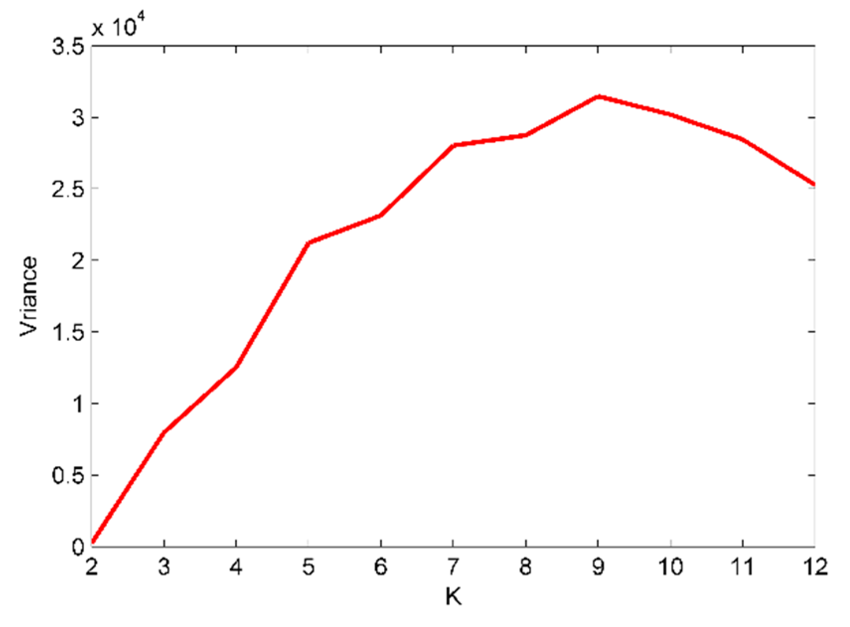
- Based on the center frequency of the intrinsic mode functions, the variational mode decomposition mode number will be calculated firstly.
- (2)
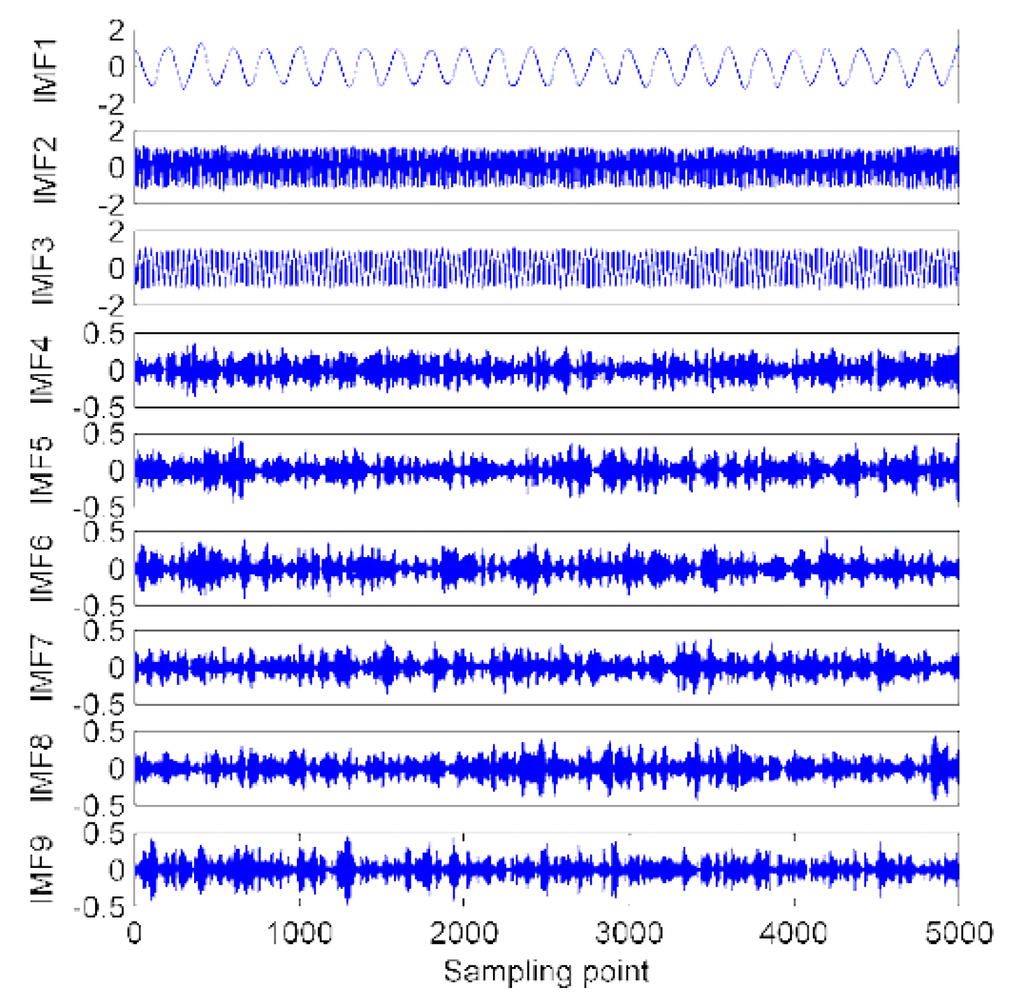
- The VMD algorithm based on the optimum mode number obtained in the first step is applied to the decomposition of the SRN signals.
- (3)
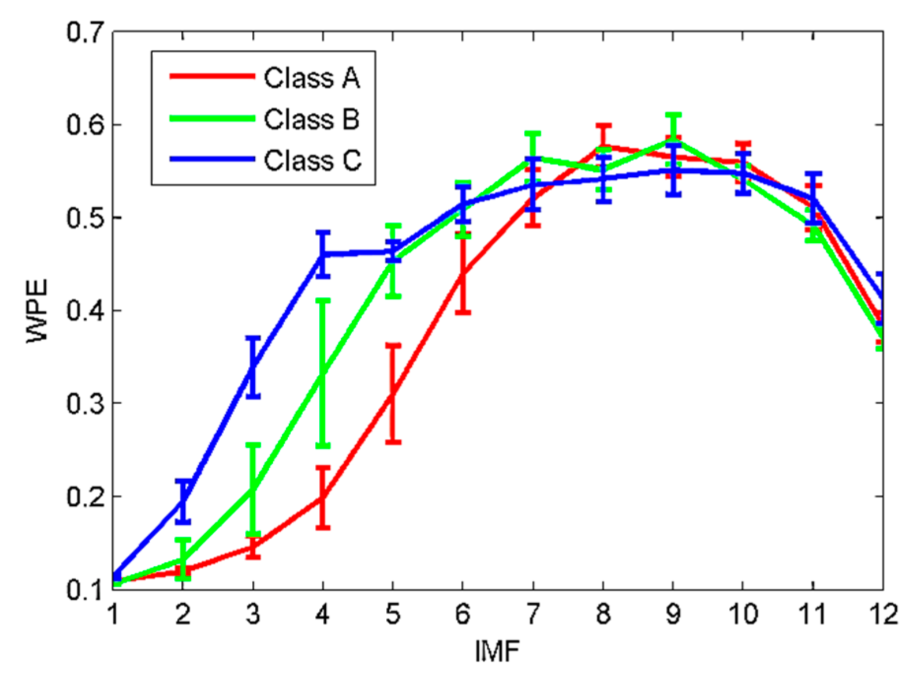
- The WPE of each IMF by EVMD is then calculated.
- (4)
- The feature vectors obtained will be randomly divided into two groups, the first group represent the training data used in classification information while the second one is used for evaluating the testing data and measuring its ability for classification.
- (5)
- Definitively, PSO-SVM multiclass classifier uses the analysis data that are recognized and detects the underwater acoustic object.
4. Simulation Signals Analysis
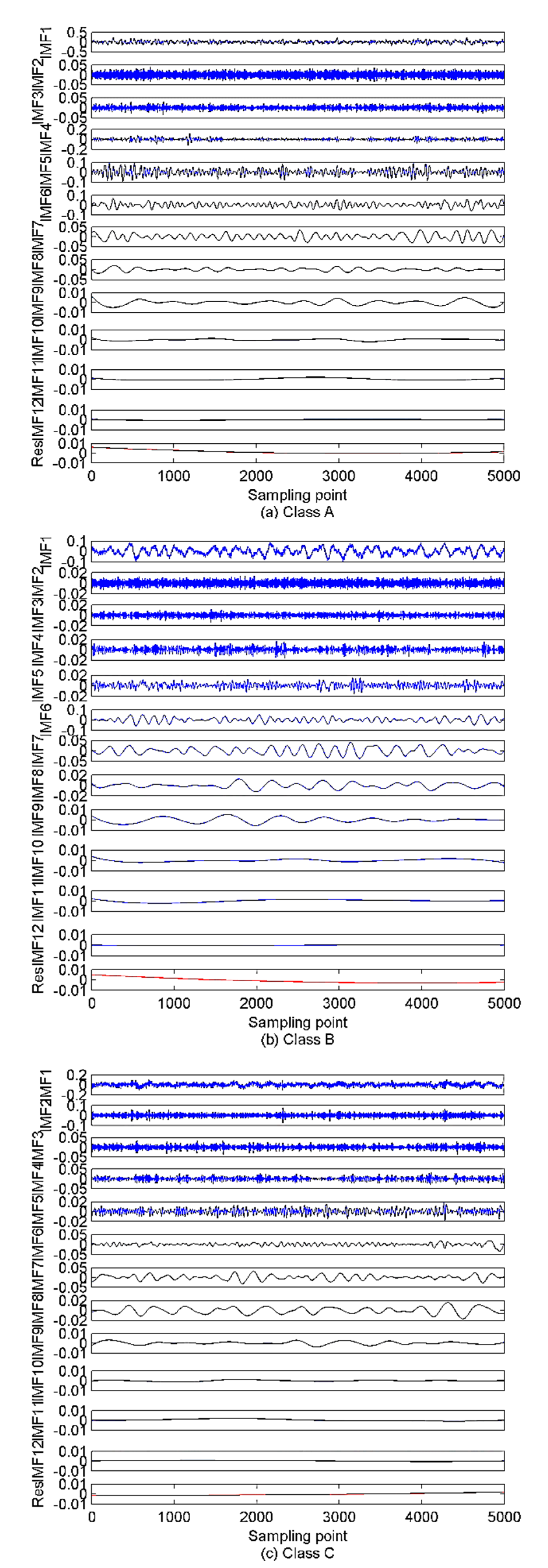
4.1. Analysis of Simulated Signals Based on EVMD
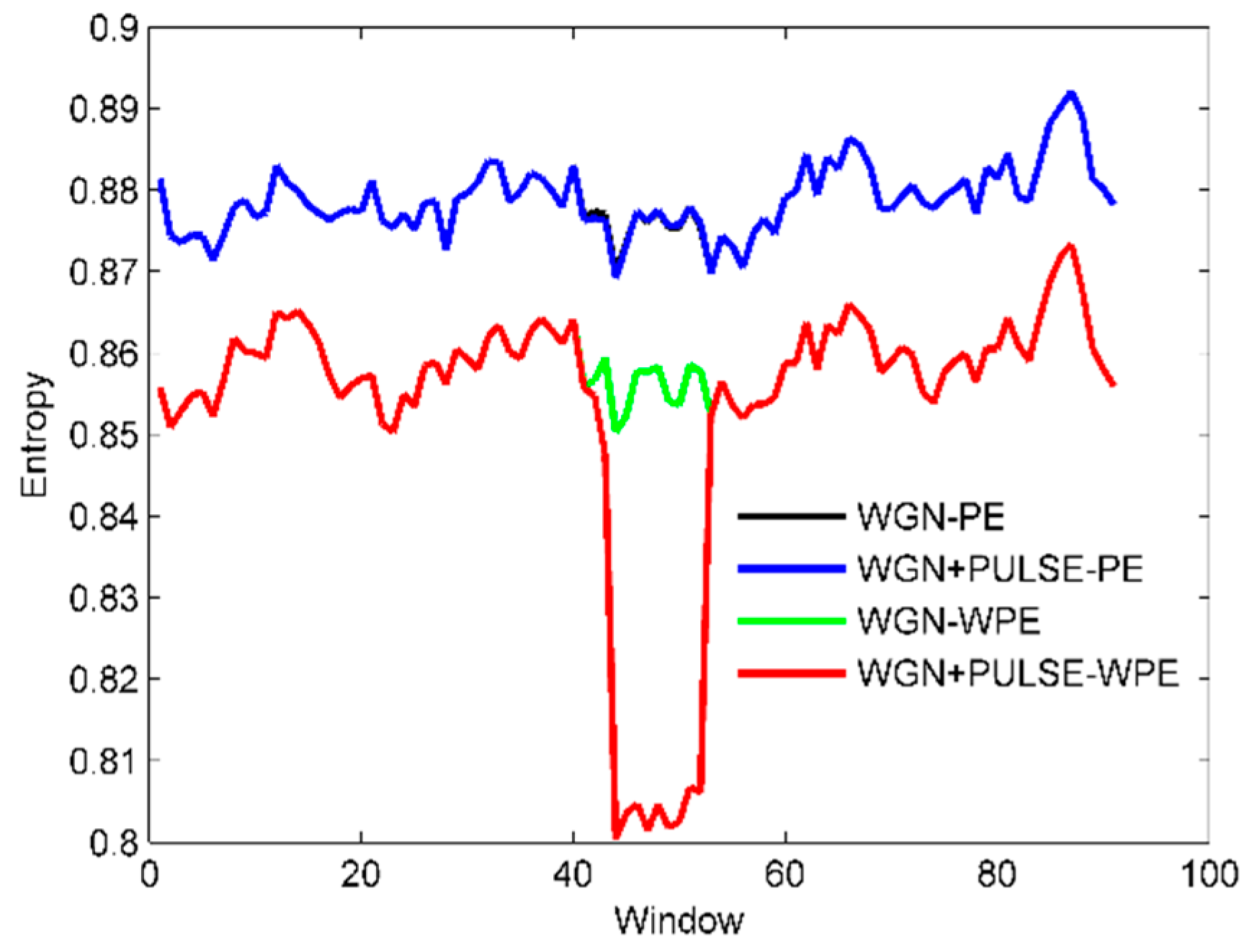
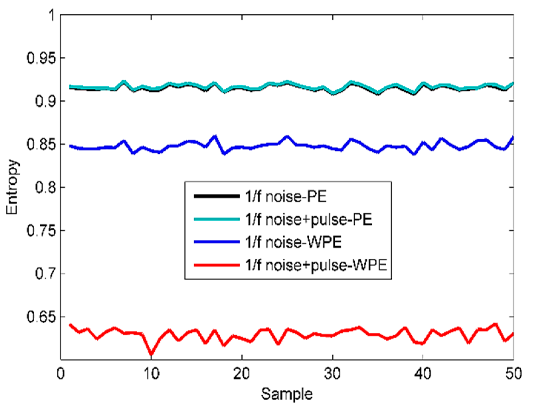
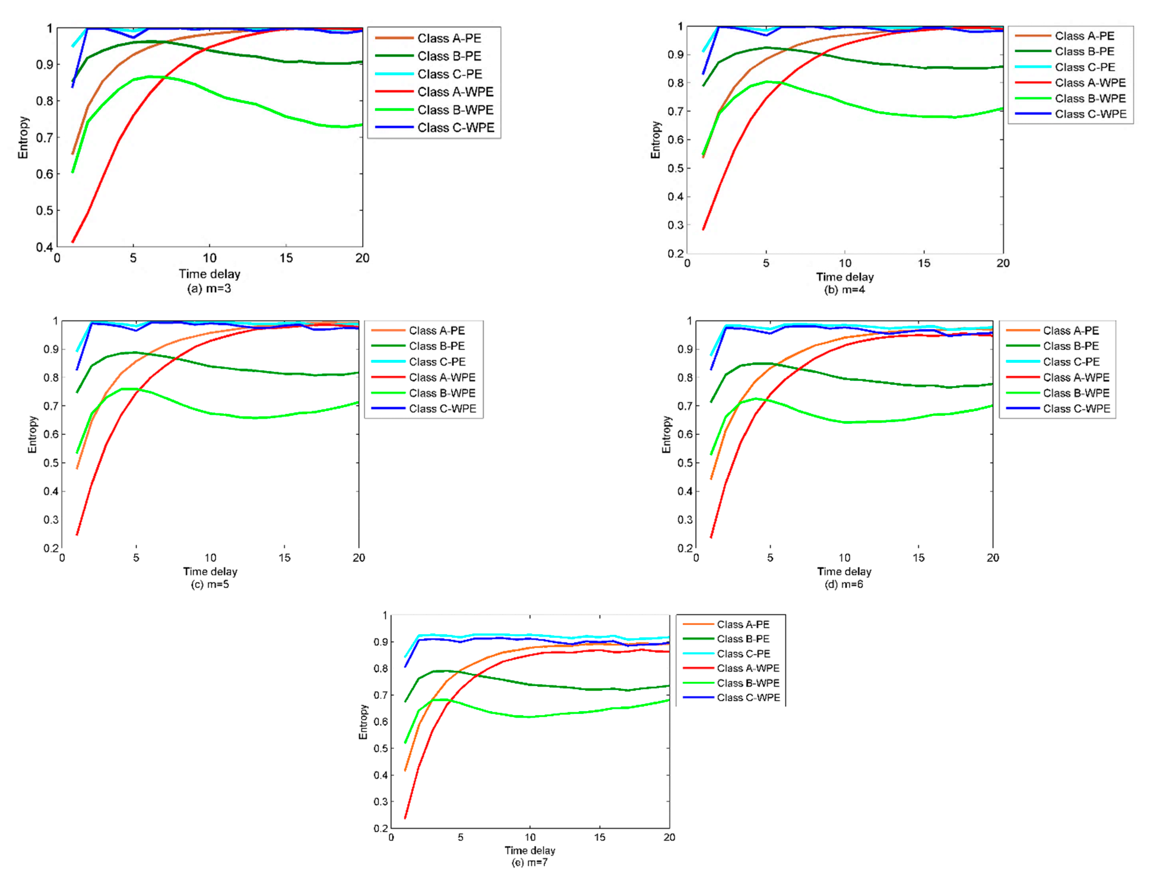
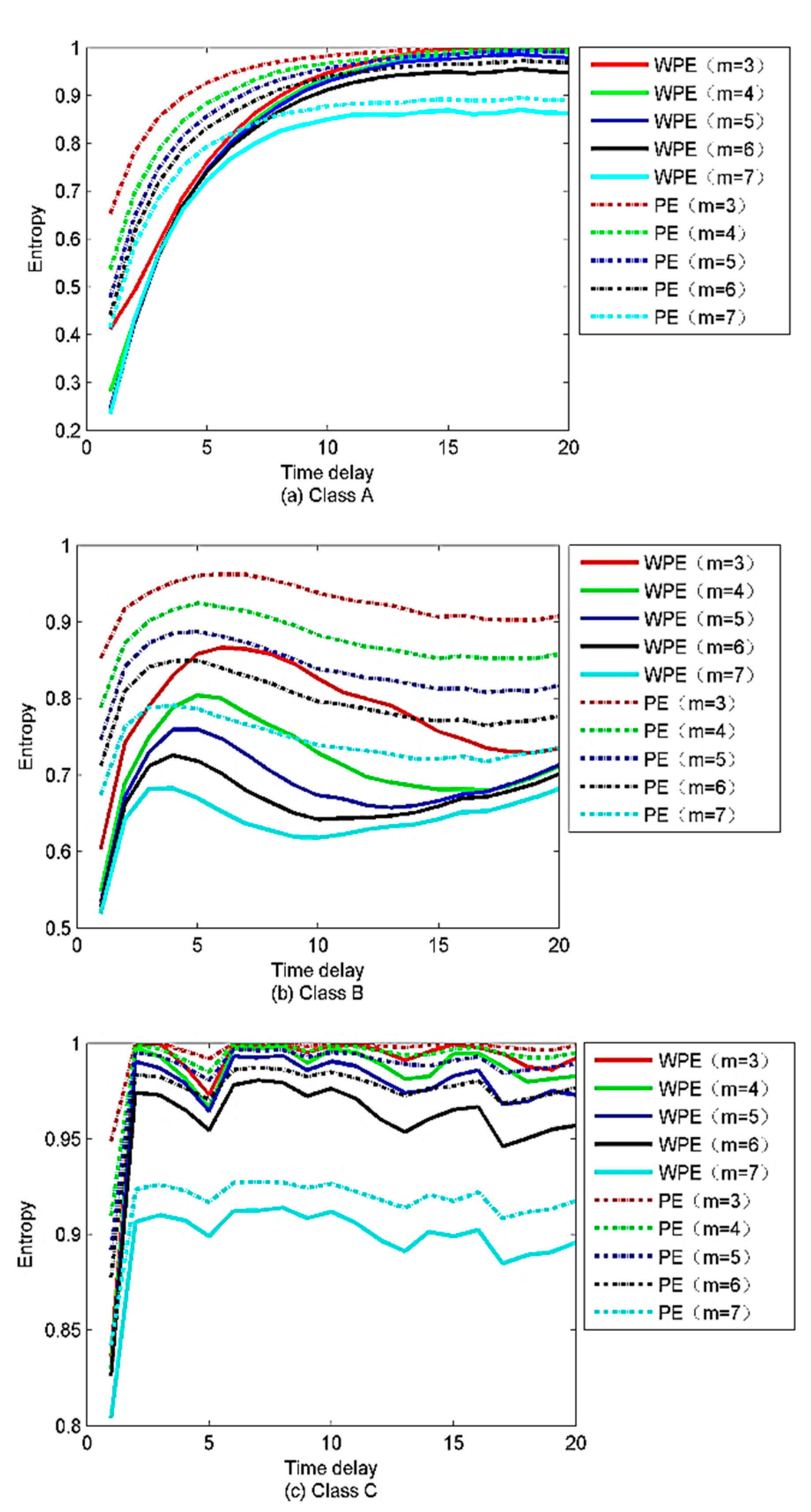
4.2. Analysis of the Properties Concerning Weighted Permutation Entropy (WPE) and Permutation Entropy (PE)
5. Feature Extraction of Ship-Radiated Noise Based on the Proposed Method
5.1. Parameter Selection
5.2. Decomposition of Ship-Radiated Noise Using VMD
5.3. Classification of Ship-Radiated Noise (SRN)
6. Conclusions
- (1)
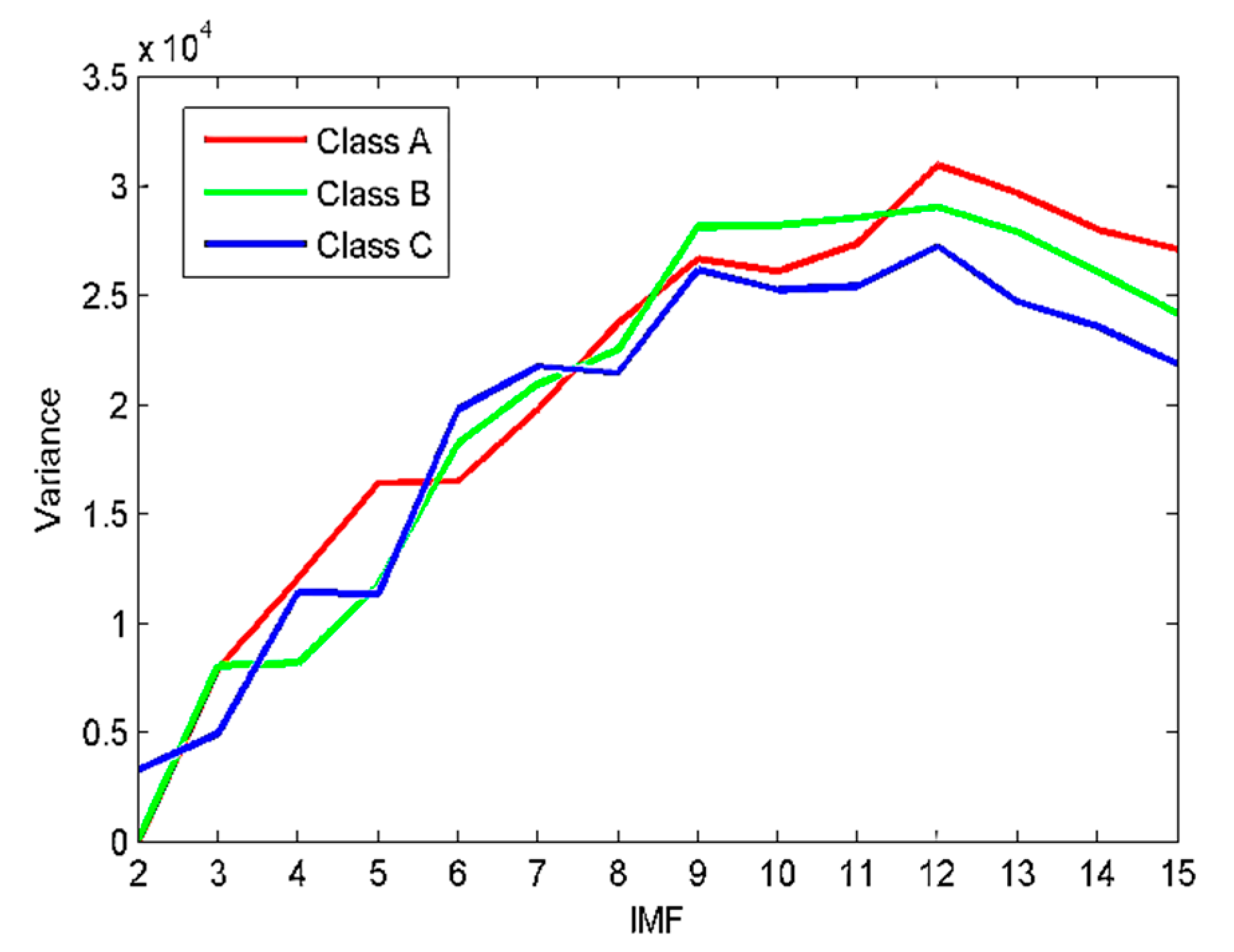
- The proposed EVMD method mode number was calculated based on the variance of IMFs’ center frequency.
- (2)
- WPE and LTSA were combined with the new EVMD and applied to underwater SRN signals for the first time.
- (3)
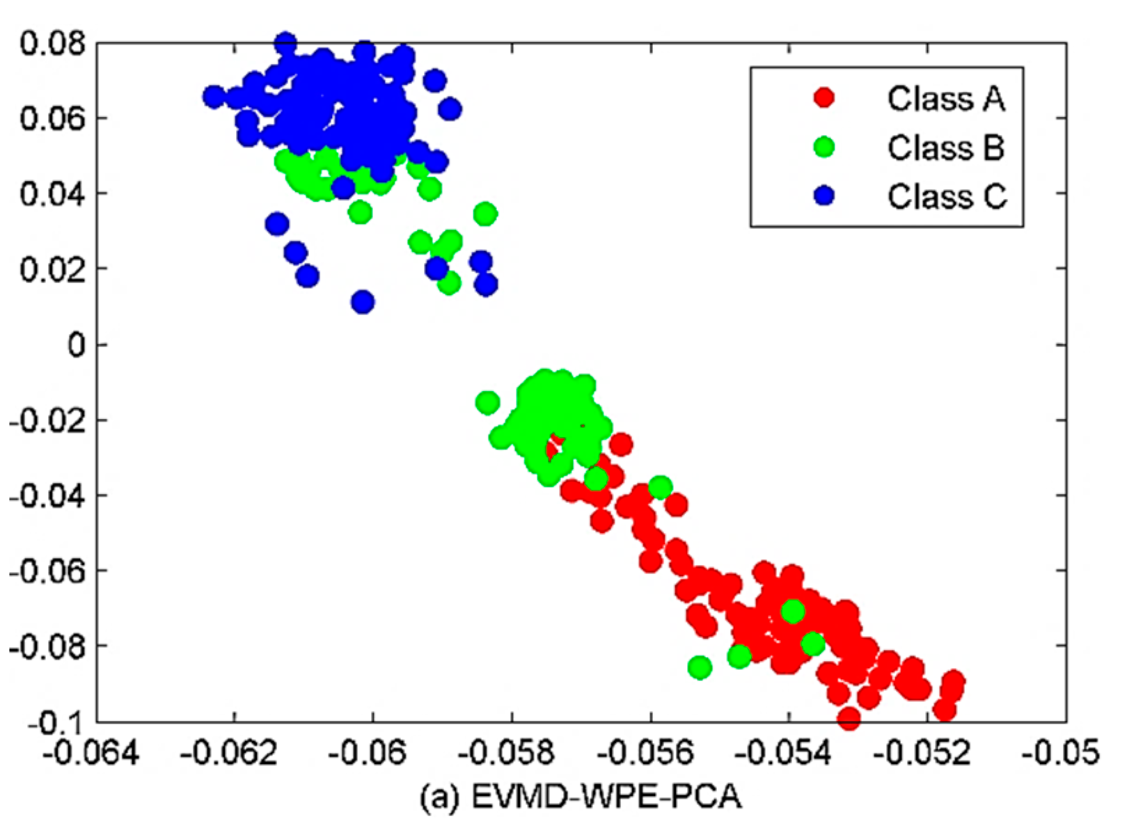
- The proposed EVMD-WPE-LTSA was successfully applied, and extracted the features of the underwater acoustic signals. Compared with other algorithms, EVMD-WPE-LTSA had a higher recognition rate and better classification performance at the cost of computational time.
Author Contributions
Funding
Data Availability Statement
Conflicts of Interest
References
- Xie, D.; Esmaiel, H.; Sun, H.; Qi, J.; Qasem, Z.A. Feature Extraction of Ship-Radiated Noise Based on Enhanced Variational Mode Decomposition, Normalized Correlation Coefficient and Permutation Entropy. Entropy 2020, 22, 468. [Google Scholar] [CrossRef] [PubMed] [Green Version]
- Rao, R. Wavelet Transforms. In Encyclopedia of Imaging Science and Technology; Wiley: New York City, NY, USA, 2002. [Google Scholar]
- Huang, N.E.; Shen, Z.; Long, S.R.; Wu, M.C.; Shih, H.H.; Zheng, Q.; Yen, N.-C.; Tung, C.C.; Liu, H.H. The empirical mode decomposition and the Hilbert spectrum for nonlinear and non-stationary time series analysis. Proc. R. Soc. Lond. Ser. A Math. Phys. Eng. Sci. 1998, 454, 903–995. [Google Scholar] [CrossRef]
- Wu, Z.; Huang, N.E. Ensemble empirical mode decomposition: A noise-assisted data analysis method. Adv. Adapt. Data Anal. 2009, 1, 1–41. [Google Scholar] [CrossRef]
- Dragomiretskiy, K.; Zosso, D. Variational mode decomposition. IEEE Trans. Signal Process. 2013, 62, 531–544. [Google Scholar] [CrossRef]
- Zhang, X.; Wang, J.; Lin, L. Feature extraction of ship radited noises based on wavelet transform. Acta Acust. Peking 1997, 22, 139–144. [Google Scholar]
- Shih, M.-T.; Doctor, F.; Fan, S.-Z.; Jen, K.-K.; Shieh, J.-S. Instantaneous 3D EEG signal analysis based on empirical mode decomposition and the hilbert–huang transform applied to depth of anaesthesia. Entropy 2015, 17, 928–949. [Google Scholar] [CrossRef] [Green Version]
- Xie, P.; Yang, F.-M.; Li, X.-X.; Yang, Y.; Chen, X.-L.; Zhang, L.-T. Functional coupling analyses of electroencephalogram and electromyogram based on variational mode decomposition-transfer entropy. Acta Phys. Sin. 2016, 65, 118701. [Google Scholar]
- Taran, S.; Bajaj, V. Clustering variational mode decomposition for identification of focal EEG signals. IEEE Sens. Lett. 2018, 2, 1–4. [Google Scholar] [CrossRef]
- Hsieh, N.-K.; Lin, W.-Y.; Young, H.-T. High-speed spindle fault diagnosis with the empirical mode decomposition and multiscale entropy method. Entropy 2015, 17, 2170–2183. [Google Scholar] [CrossRef] [Green Version]
- Zhang, X.; Liang, Y.; Zhou, J. A novel bearing fault diagnosis model integrated permutation entropy, ensemble empirical mode decomposition and optimized SVM. Measurement 2015, 69, 164–179. [Google Scholar] [CrossRef]
- Lei, Y.; He, Z.; Zi, Y. Application of the EEMD method to rotor fault diagnosis of rotating machinery. Mech. Syst. Signal Process. 2009, 23, 1327–1338. [Google Scholar] [CrossRef]
- Li, Y.; Li, Y.; Chen, X.; Yu, J. A novel feature extraction method for ship-radiated noise based on variational mode decomposition and multi-scale permutation entropy. Entropy 2017, 19, 342. [Google Scholar] [CrossRef] [Green Version]
- Yang, H.; Zhao, K.; Li, G. A new ship-radiated noise feature extraction technique based on variational mode decomposition and fluctuation-based dispersion entropy. Entropy 2019, 21, 235. [Google Scholar] [CrossRef] [PubMed] [Green Version]
- Bandt, C.; Pompe, B. Permutation entropy: A natural complexity measure for time series. Phys. Rev. Lett. 2002, 88, 174102. [Google Scholar] [CrossRef] [PubMed]
- Tian, Y.; Wang, Z.; Lu, C. Self-adaptive bearing fault diagnosis based on permutation entropy and manifold-based dynamic time warping. Mech. Syst. Signal Process. 2019, 114, 658–673. [Google Scholar] [CrossRef]
- de Araujo, F.H.A.; Bejan, L.; Rosso, O.A.; Stosic, T. Permutation entropy and statistical complexity analysis of Brazilian agricultural commodities. Entropy 2019, 21, 1220. [Google Scholar] [CrossRef] [Green Version]
- Henry, M.; Judge, G. Permutation entropy and information recovery in nonlinear dynamic economic time series. Econometrics 2019, 7, 10. [Google Scholar] [CrossRef] [Green Version]
- Li, R.; Wang, J. Interacting price model and fluctuation behavior analysis from Lempel–Ziv complexity and multi-scale weighted-permutation entropy. Phys. Lett. A 2016, 380, 117–129. [Google Scholar] [CrossRef]
- Fadlallah, B.; Chen, B.; Keil, A.; Príncipe, J. Weighted-permutation entropy: A complexity measure for time series incorporating amplitude information. Phys. Rev. E 2013, 87, 022911. [Google Scholar] [CrossRef] [Green Version]
- Wu, E.Q.; Zhu, L.-M.; Zhang, W.-M.; Deng, P.-Y.; Jia, B.; Chen, S.-D.; Ren, H.; Zhou, G.-R. Novel Nonlinear Approach for Real-Time Fatigue EEG Data: An Infinitely Warped Model of Weighted Permutation Entropy. IEEE Trans. Intell. Transp. Syst. 2019, 21, 2437–2448. [Google Scholar] [CrossRef]
- Wu, P.; Guo, L.; Duan, Y.; Zhou, W.; He, G. Control loop performance monitoring based on weighted permutation entropy and control charts. Can. J. Chem. Eng. 2019, 97, 1488–1495. [Google Scholar] [CrossRef]
- Wold, S.; Esbensen, K.; Geladi, P. Principal component analysis. Chemom. Intell. Lab. Syst. 1987, 2, 37–52. [Google Scholar] [CrossRef]
- Reza, M.S.; Ma, J. ICA and PCA Integrated Feature Extraction for Classification. In Proceedings of the IEEE 13th International Conference on Signal Processing (ICSP), Chengdu, China, 6–10 November 2016. [Google Scholar]
- Tharwat, A.; Gaber, T.; Ibrahim, A.; Hassanien, A.E. Linear discriminant analysis: A detailed tutorial. AI Commun. 2017, 30, 169–190. [Google Scholar] [CrossRef] [Green Version]
- Zhang, Z.; Zha, H. Principal Manifolds and Nonlinear Dimension Reduction via Local Tangent Space Alignment; Tech Rep CSE-02-019; Department of Computer Science, Pennsylvania State University: University Park, PA, USA, 2002. [Google Scholar]
- Ma, P.; Zhang, H.; Fan, W.; Wang, C. Early fault detection of bearings based on adaptive variational mode decomposition and local tangent space alignment. Eng. Comput. 2019, 36, 509–532. [Google Scholar] [CrossRef]
- Li, S.; Qian, P.; Gu, H. Fault Detection of Discriminant Improved Local Tangent Space Alignment. In Proceedings of the International Conference on Intelligent Informatics and Biomedical Sciences (ICIIBMS), Shanghai, China, 21–24 November 2019. [Google Scholar]
- Ye, Y.; Zhang, Y.; Wang, Q.; Wang, Z.; Teng, Z.; Zhang, H. Fault diagnosis of high-speed train suspension systems using multiscale permutation entropy and linear local tangent space alignment. Mech. Syst. Signal Process. 2020, 138, 106565. [Google Scholar] [CrossRef]
- Zhang, N.; Sun, Y.; Zhang, Y.; Yang, P.; Lin, A.; Shang, P. Distinguishing Stock Indices and Detecting Economic Crises Based on Weighted Symbolic Permutation Entropy. Fluct. Noise Lett. 2019, 18, 1950026. [Google Scholar] [CrossRef]
- Zheng, J.; Pan, H.; Yang, S.; Cheng, J. Generalized composite multiscale permutation entropy and Laplacian score based rolling bearing fault diagnosis. Mech. Syst. Signal Process. 2018, 99, 229–243. [Google Scholar] [CrossRef]
- Santos-Domínguez, D.; Torres-Guijarro, S.; Cardenal-López, A.; Pena-Gimenez, A. ShipsEar: An underwater vessel noise database. Appl. Acoust. 2016, 113, 64–69. [Google Scholar] [CrossRef]


| Center Frequency/Hz | ||||||||||||
|---|---|---|---|---|---|---|---|---|---|---|---|---|
| 2 | 7.79 | 52.50 | ||||||||||
| 3 | 7.77 | 52.50 | 310.22 | |||||||||
| 4 | 7.73 | 52.51 | 193.88 | 358.92 | ||||||||
| 5 | 7.71 | 52.52 | 178.13 | 306.10 | 429.27 | |||||||
| 6 | 7.63 | 52.53 | 132.93 | 231.63 | 325.67 | 438.33 | ||||||
| 7 | 5.04 | 55.14 | 30.02 | 178.15 | 281.03 | 365.89 | 468.10 | |||||
| 8 | 5.04 | 55.12 | 30.02 | 150.48 | 230.17 | 304.96 | 377.06 | 470.06 | ||||
| 9 | 5.04 | 55.11 | 30.02 | 133.53 | 202.41 | 280.99 | 349.96 | 413.83 | 476.09 | |||
| 10 | 5.04 | 55.09 | 30.01 | 122.45 | 181.76 | 240.15 | 300.08 | 359.29 | 418.56 | 477.08 | ||
| 11 | 5.03 | 55.09 | 30.01 | 118.11 | 173.42 | 227.27 | 276.65 | 321.81 | 369.88 | 424.40 | 478.29 | |
| 12 | 5.03 | 55.05 | 30.01 | 99.61 | 146.79 | 192.70 | 237.79 | 283.66 | 325.96 | 372.20 | 425.66 | 468.56 |
| EMD | EEMD | VMD | EVMD | |
|---|---|---|---|---|
| f1 | IMF6: 0.9244 | IMF7: 0.9665 | IMF1: 0.9938 | IMF1: 0.9944 |
| f2 | IMF4: 0.8959 | IMF5: 0.9806 | IMF3: 0.9914 | IMF3: 0.9925 |
| f3 | IMF3: 0.8875 | IMF4: 0.9460 | IMF2: 0.9872 | IMF2: 0.9880 |
| Method | NUMBER OF MISCLASSIFIED SAMPLES | ACCURACY RATE (%) | COMPUTATIONAL TIMES (SECOND) | ||
|---|---|---|---|---|---|
| CLASS A | CLASS B | CLASS C | |||
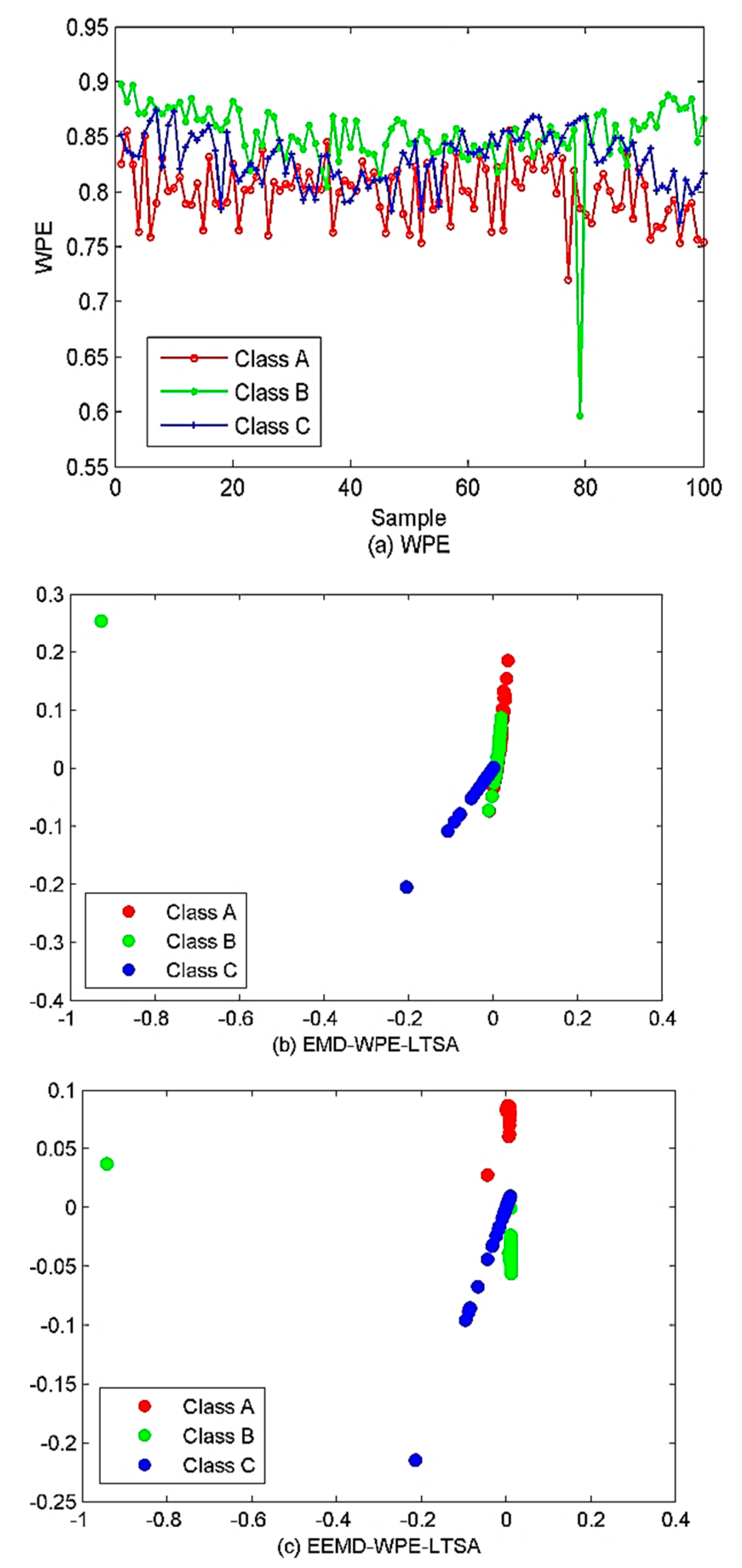
| WPE | 11 | 7 | 27 | 62.5 | 787.35041 |
| EMD-WPE-LTSA | 11 | 9 | 2 | 81.6667 | 6956.81681 |
| EEMD-WPE-LTSA | 0 | 12 | 0 | 90 | 23,643.2661 |
| EVMD-WPE-PCA | 2 | 5 | 5 | 90 | 22,254.0133 |
| EVMD-WPE-MDS | 4 | 2 | 0 | 95 | 22,255.2634 |
| EVMD-WPE-LLE | 1 | 4 | 0 | 95.8333 | 22,255.0276 |
| EVMD-WPE-LTSA | 3 | 0 | 1 | 96.6667 | 22,255.0041 |
| EMD-EIMF-PE | 5 | 0 | 8 | 89.1667 | 1342.94618 |
| VMD-WPE-LTSA | 3 | 5 | 0 | 93.3333 | 12,404.5999 |
Publisher’s Note: MDPI stays neutral with regard to jurisdictional claims in published maps and institutional affiliations. |
© 2021 by the authors. Licensee MDPI, Basel, Switzerland. This article is an open access article distributed under the terms and conditions of the Creative Commons Attribution (CC BY) license (https://creativecommons.org/licenses/by/4.0/).
Share and Cite
Esmaiel, H.; Xie, D.; Qasem, Z.A.H.; Sun, H.; Qi, J.; Wang, J. Multi-Stage Feature Extraction and Classification for Ship-Radiated Noise. Sensors 2022, 22, 112. https://doi.org/10.3390/s22010112
Esmaiel H, Xie D, Qasem ZAH, Sun H, Qi J, Wang J. Multi-Stage Feature Extraction and Classification for Ship-Radiated Noise. Sensors. 2022; 22(1):112. https://doi.org/10.3390/s22010112
Chicago/Turabian StyleEsmaiel, Hamada, Dongri Xie, Zeyad A. H. Qasem, Haixin Sun, Jie Qi, and Junfeng Wang. 2022. "Multi-Stage Feature Extraction and Classification for Ship-Radiated Noise" Sensors 22, no. 1: 112. https://doi.org/10.3390/s22010112
APA StyleEsmaiel, H., Xie, D., Qasem, Z. A. H., Sun, H., Qi, J., & Wang, J. (2022). Multi-Stage Feature Extraction and Classification for Ship-Radiated Noise. Sensors, 22(1), 112. https://doi.org/10.3390/s22010112