Abstract
This paper present simulation-based results on the impact of transmitter (Tx) position and orientation uncertainty on the accuracy of the visible light positioning (VLP) system based on the received signal strength (RSS). There are several constraining factors for RSS-based algorithms, particularly due to multipath channel characteristics and set-up uncertainties. The impact of Tx uncertainties on positioning error performance is studied, assuming a statistical modelling of the uncertainties. Simulation results show that the Tx uncertainties have a severe impact on the positioning error, which can be leveraged through the usage of more transmitters. Concerning a smaller Tx’s position uncertainty of 5 cm, the average positioning errors are 23.3, 15.1, and 13.2 cm with the standard deviation values of 6.4, 4.1, and 2.7 cm for 4-, 9-, and 16-Tx cases, respectively. While for a smaller Tx’ orientation uncertainty of 5°, the average positioning errors are 31.9, 20.6, and 17 cm with standard deviation values of 9.2, 6.3, and 3.9 cm for 4-, 9-, and 16-Tx cases, respectively.
1. Introduction
The demand for highly precise indoor positioning (IP) systems is growing rapidly due to its potential in the increasingly popular techniques of Internet of Thing (IoT), smart mobile devices, and artificial intelligence. Consequently, IP becomes a promising research domain that is getting wide attention due to its benefits in several working scenarios, such as, industries, health sectors, indoor public locations, and autonomous navigation [1]. The traditional positioning methods, which depend on satellites such as the global positioning system (GPS), is common nowadays for outdoor positioning; however, it is not well-suited for indoor environments. This is because the GPS signals from the satellites suffer from high penetration loss and multipath fading due to building walls. Some other systems also have been proposed for IP, for example, Bluetooth, ultrasound, ultra-wideband (UWB), wireless-Fidelity, radio frequency identification (RFID), and radio-frequency (RF)-based techniques [2,3,4]. For instance, the UWB technology transmits short RF pulses with a low duty cycle, which provides precise localization and tracking of mobile devices in indoor environments [4]. Despite the advantage of precise localization, the UWB technology is still not perfect for IP systems, and it has not been embraced widely because of its cost, complexity, and need for synchronization between transmitters (Txs) and the targets [5]. Moreover, these RF-based systems may not be suitable in RF restricted areas, such as hospitals due to the RF-induced interference [2].
Another developed technology that makes use of the pre-installed lighting infrastructure is visible light positioning (VLP). VLP is based on visible light communications (VLC), which is license-free, and free from RF induced electromagnetic interference-free, thus making it ideal in many applications including hospitals. In addition, VLC uses the pre-existing light-emitting diodes (LEDs) infrastructure as a Tx which has the ability to provide illuminance and communication simultaneously [6]. VLP is an emerging technology promising high accuracy, high security, low deployment cost, shorter time response, and low relative complexity when compared with RF-based positioning [7].
Existing VLP approaches estimate the position of a receiver (Rx) based on several characteristics of light including received signal strength (RSS) [8], angle of arrival (AOA)/angle difference of arrival (ADOA) [9], image [10], and time of arrival (TOA)/time difference of arrival (TDOA) [11]. It has been established that, VLP based on AOA/ADOA, image, and TOA/TDOA require auxiliary devices to capture angle/image/time. On the contrary, the RSS approach can be achieved by utilizing a single photodiode (PD) without the need of any additional auxiliary devices, which makes the RSS-based approach the most well-known method for VLP [12].
Recent research works have addressed the impact of (i) LED power uncertainty [13]; (ii) reflections from walls and objects within the transmission paths [14]; and (iii) noise on the positioning performance [15]. The multipath channel has a direct influence on the model for the estimation of the received signal power, which has been addressed previously using machine learning algorithms [16]. The Tx and the Rx design specifications, such as the Tx beam width and its tilting angle have been investigated before. For instance, in [13], the impact of LED output power uncertainty on the accuracy of the RSS-based VLP system was explored, with the maximum error of 17 and 40 cm for a tolerance (possible variations) value of 5% and 20%, respectively. The performance analysis of various VLP systems relies on line-of-sight (LOS) transmission path, which can underestimate the achievable error bounds, due to the fact that a real scenario will definitely include non-line of sight (NLOS) paths [14]. Therefore, NLOS transmission paths should not be neglected. In [15], an RSS-based VLP system using received optical power from the emitting LEDs was investigated considering signals from both LOS and NLOS paths. The results revealed that, the positioning accuracy of <10 cm on average can be achieved at a signal-to-noise ratio (SNR) of >12 dB.
The location of the Rx can be estimated by using different estimation methods, such as linear least square (LLS) and non-linear least square (NLLS) [14]. In [17], a polynomial regression-based method was used to investigate the accuracy of an RSS-based VLP system along with LLS and NLLS estimation algorithms. The results revealed that, the positioning error εp was <0.6 m by using the regression approach, which is much lower than other traditional methods. In [18], the impact of the Tx’s orientation (i.e., the tilting angle) on the positioning accuracy of the RSS-based VLP system was studied. Another estimation method, i.e., normalized least square estimation was utilized to estimate the positioning accuracy. In [19], an artificial neural network (ANN) based 4-LED VLP system was proposed to reduce εp for the LOS path, which is affected by the random and unknown static Tx tilt angle with a maximum variation of 2°. It was revealed that ANN achieved localization errors below 1 cm. In general, the positions and orientations of Txs may not be symmetrical, which (i) depends on the indoor environments such as museums, galleries, train stations, shopping centers, etc., where lights are pointing in different directions; and (ii) can change when replacing lights, carrying out maintenance, etc. Therefore, the random variations in the Tx’s orientation will lead to the random errors in VLP systems, which requires further studies. The impact of Tx’s position and its orientation uncertainties on the positioning estimation have not yet been systematically explored, which is the objective of this paper.
In this paper, we investigate the impact of Tx’s position and its orientation uncertainties on εp of the RSS-based VLP system under multipath reflections. The uniform distribution of light inside the illuminated place is a necessity in indoor environments. As a result, lighting uniformity becomes a vital aspect for a well-lit environment. Moreover, both lighting uniformity and the positioning performance are related to the Tx’s positions and the Lambertian half-power angles (HPA). Therefore, in this work we investigate (i) how the uniformity of light in the room changes for different HPA and the Tx positions; and (ii) the impact of Tx position and its orientation uncertainties on the positioning accuracy considering the optimized Tx positions from a lighting uniformity perspective. This works focused only on the LED uncertainties caused during installation and is an extension of our previous work [20], where the problem of Tx’s orientation uncertainty was not considered.
The rest of the paper is organized as follows, Section 2 introduces the set-up of the system and position estimation approaches in detail. The impact of different set-up uncertainties and uniformity are presented in Section 3. In Section 4, a discussion of the simulation results attained is made, followed by the final concluding remarks in Section 5.
2. VLP System Modelling
2.1. Channel Model
Our proposed VLP system is composed of a PD as an Rx, which is placed on the ground and a number of LEDs as the Txs (i.e., 4-, 9-, and 16-LED) that are installed on the ceiling of the room as depicted in Figure 1. The field of view (FOV) and the detection area Ar of the PD are 70° and 10−4 m2, respectively. All Txs are located at the same height h from the ground level and the coordinates of kth Tx (k = 1, …, K) is (), where K is the total number of Txs. The Rx coordinate is denoted by (). The position and orientation of the Txs is best illustrated by the , with the coordinate of () and the angles of , , and . Both and , and , , and , are assumed to be Gaussian variables with N(0, ) and N(0, ζ2) probability distribution functions, respectively. The distance between the Txs relies on the lighting uniformity considerations that are described in a later section. An empty room is considered as a reference to study the impact of Tx’s position and its orientation uncertainty on the positioning accuracy. In this work, both LOS and NLOS transmission paths are assumed between the Txs and the Rx. However, for the NLOS path, we only consider the first reflection due to the fact that the second order reflections have much reduced intensities and therefore can be neglected [21]. Each Tx broadcast a unique 2-bit ID information, which is encoded and modulated using on-off keying (OOK), which allows separation at the Rx using a correlation method that can be received at the Rx in advance of location identification.
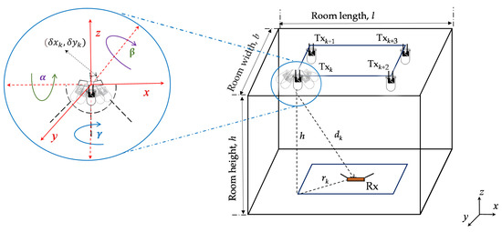
Figure 1.
Overview of the simulation set-up.
The total received optical power at the PD comprises the power from the LOS and NLOS paths, as given by:
where and represent the received power for LOS and NLOS, respectively. Generally, the SNR will be high (i.e., >20 dB) in standard VLC, which could be considered noise-free in normal cases [22]. Thus, in this study, no actual noise (e.g., shot noise or thermal noise) is considered as a source of “measurement noise”, to unambiguously evaluate the effect of the Tx’s position and its orientation uncertainty.
2.2. RSS-Based Positioning
Using the RSS algorithm, for the LOS path can be expressed as [22,23]:
where
where is the transmit power, is the distance between kth Tx and the Rx, K is the total number of Txs, and is the light source irradiance half-power angle (HPA) [22]. and φ are the irradiance angle from the kth Tx to the Rx and the receiving incident angle, respectively. Ar and are the PD’s active area and responsivity, respectively. and are the gains of the optical filter and the concentrator at the Rx, respectively. Note, and are set to unity.
Considering the NLOS path, i.e., the first-order reflection, the total received power can be expressed as [22]:
where , , and are the distances, receiving incident angle, and the irradiance angle between the kth Tx and the reflective area, respectively. , , and are the distances, receiving incident angle, and the irradiance angle between the reflective area and the Rx, respectively, see Figure 2. ρ is the reflection coefficient that relies on the reflective surface material, and is the reflection area. for the signals from the NLOS paths is obtained based on Matlab [22]. For each Tx, we integrate (4) over all the walls accompanied by the assumption of a grid area with a resolution of 0.1 m.
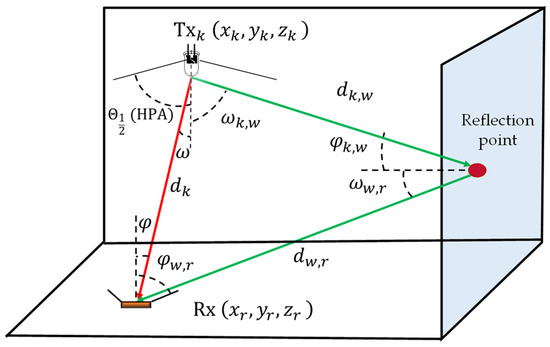
Figure 2.
Overview of the visible light channel.
2.3. Distance Estimation Using Polynomial Regression
The block diagram of the proposed VLP system is shown in Figure 3. In the case of LOS, the horizontal distance can be computed as and therefore can be determined from (2) as given by:
where h is the vertical distance between the Tx and the Rx. is the LOS received power at the Rx from the kth Tx. In (5), the cosine terms are clearly stated in terms of the set-up geometry, as . However, in case of NLOS links, high errors are introduced in the channel due to the presence of reflections [17,24], thus, the above method fails to determine the distance. Another method that can be used is to employ a polynomial fitted model for the power-distance relationship [25]. In this particular case, the relation between and for the kth Tx is represented as:
where is the total received power at the Rx from the kth Tx, and represent the coefficients of the fitted polynomial. Note, is computed using (6), which is later employed to determine .
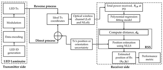
Figure 3.
Block diagram of the proposed system.
We estimated the best polynomial fitting using 3600 data points extracted from channel simulation, see Figure 4. Note that, the 3600 data points are considered as 3600 different locations each within the room. The best-fitted solution was exhibited by analyzing the value of R2 (coefficient of determination) for different orders, and a fourth order polynomial was selected with a value of R2 of 0.8942. Note, the polynomial fitting is not highly accurate. This is because of the data points considered within the entire room for both LOS and NLOS paths. At the center of the room, the impact of NLOS is negligible when compared to the regions near walls and corners. As such, fitting all the data will be dominated by the data near walls and corners. However, it shows the best fitted solution considering that the data points corresponding to lower received power have higher contributions to the error compared with the data points in the center of the room. The values of polynomial coefficients are listed in Table 1.
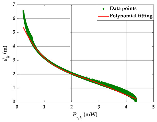
Figure 4.
Estimation using the polynomial fitting method.

Table 1.
The value of polynomial coefficients for the best polynomial fitting.
2.4. Estimation Using Nonlinear Least Squares
The relation between the Tx coordinates () and the Rx coordinates () are described using the following equations:
where K is the total number of Txs. NLLS estimation can be utilized to estimate the target location, in which the solution can be estimated by attaining that minimizes a cost function given by [15]:
An iterative procedure is utilized to estimate by employing the trust-region reflective algorithm [26]. In this algorithm, first, an estimate is introduced as , followed by computing the corresponding cost function . Next, several points in the neighborhood of are replaced in (8), and the one that minimizes the cost is selected as . The Rx coordinates will eventually be obtained following several iterative steps to ensure convergence of . In the proposed system, the initial value for is estimated using a linear least square approach.
2.5. Performance Metrics
εp is assumed to be a random variable (as it may rely on the uncertainties, i.e., the Tx’s position or its orientation uncertainties, estimation process, or noise); thus, it is reasonable to use the standard statistical analyses to access error performance. Here we use the probability distribution function (PDF) and the cumulative distribution function (CDF), as a mean to calculate the 95% quantile on εp. Hence, the PDF and CDF are composed of the spatial distribution of εp within the entire room. The PDF of εp is defined as:
where ε defines an error interval centered around p, and N is the number of samples. The cardinal operator # signifies the counting of occurrences were |-p| < ε. The limiting process is naturally implied by the discrete nature of the simulation. The CDF can be expressed as:
Figure 5 depicts the CDF against εp for NLLS estimation with and without polynomial regression. The maximum εp values estimated by NLLS and NLLS with polynomial regression are 0.6 and 1.57 m, respectively. It is observed that, there is an evident improvement in the positioning accuracy by using NLLS estimation with polynomial regression for power-distance modeling. Therefore, the polynomial regression can improve the accuracy of position estimation without the inclusion of high complexity algorithms. However, there are some limitations of the polynomial regression; for instance, the coefficients of the polynomial model must be provided along with the Tx’s positions in practical scenarios. Moreover, the polynomial model can deal with the empty and non-empty rooms with the fixed furniture and objects, but with no user’s mobility.
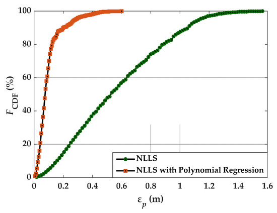
Figure 5.
CDF of the εp computed by NLLS and NLLS with polynomial regression estimation.
3. Set-Up Uncertainties
The major challenge in studying the Tx’s position or orientation uncertainties occurs in simulation, i.e., we must use random Tx positions in order to investigate the uncertainties. This raises the necessity to re-simulate the channel for each iteration (new random TX position). Give that the channel estimation is by itself complex and time-consuming, this problem becomes complex. We have developed two approaches for both Tx’s position and its orientation uncertainties to fully analyze the problem, which is termed direct and reverse processes. The reason for these designations is straightforward. The direct process entails the estimation of the position given the effect of the uncertainties on the channel. It is in this sense, complex and time-consuming. In the reverse process, the channel is assumed fixed and the effects of the Tx uncertainties are coupled directly into the estimation equations, this avoids the channel simulation at each set of newly generated Tx positions.
3.1. Uncertainties of the Tx’s Position
For Tx’s position uncertainties, in the direct process, we assume that the channel is re-stimulated for each newly generated set of Tx positions. The Tx positions are composed by the ideal position (fixed) and a random perturbation in two-dimensions. While in the reverse process, we assume that the channel is fixed for a set of ideal Tx positions, and the uncertainties are directly coupled into the estimation Equation (7). To illustrate the concept, let us consider one of the terms in (7), in the direct process, the effect of the uncertainties is on the right side of the equation, as follows:
where () and () are the coordinates of the Rx and the Tx (ideal positions), respectively. () express the uncertainty at the Tx coordinates. Both and are assumed to be Gaussian variables with N(0, ). The channel needs to be re-simulated at each iteration in order to obtain fR.
In the reverse process, it is not required to re-simulate the channel at each iteration as the uncertainties are part of the Tx position, as follows:
Subtracting (11) and (12) and extracting the mathematical expectation of both sides gives:
where is the Tx’s uncertainty of the reverse process. The reverse process has an expectation as stated in (13), which is given by (after solving (13)):
Performing the same analysis for the direct process we have:
Here, the value of is estimated using numerical simulation, where is the Tx’s uncertainty of the direct process. Assuming that, the reverse and direct processes are equivalent, the expectation values and must be equal. In this case, it is possible to infer the relation between and . This relation can be estimated assuming that the Rx is placed at the center of the room and a single Tx is placed in a uniform grid of positions for the whole room. Using mathematical simulation, we have computed the values of for different values of , see Figure 6. Note, the two processes generate uncertainties, i.e., and and these processes would be equivalent if these uncertainties are the same for certain values of and . This indicates that, the uncertainties from the reverse process can be generated with the knowledge of the direct process as given by:
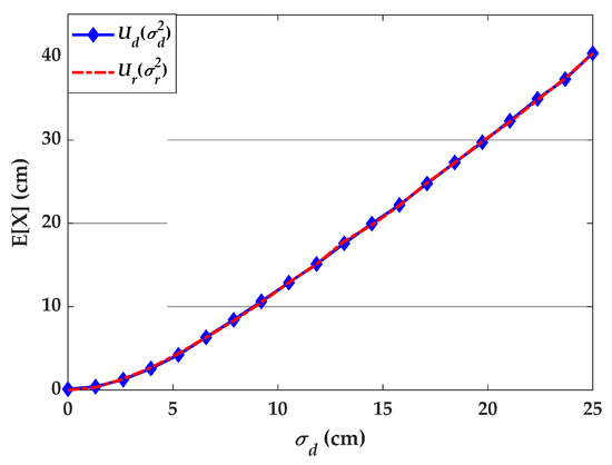
Figure 6.
Study on Tx’s position uncertainty based on the direct and reverse processes.
Simulating the uncertainty for the reverse process using the correction in (16) provides the same values for the expectation as depicted in Figure 6 (curve labelled ).
3.2. Uncertainties of the Tx’s Orientation
The Tx’s orientation uncertainties can be treated in a similar fashion as before. There are, however, some aspects that need addressing. In this paper, the Tx’ orientation uncertainties are modeled via three random axis-rotations of the Tx’s heading vector. Let us consider the kth Tx’s heading vector, , which is given by:
where , and represent the three rotation matrix relative to the x-axis, y-axis, and z-axis, respectively, , , and are three random angles with probability distribution function N(0, ζ2), finally, represents the unperturbed heading vector of the kth Tx. is a composed rotation matrix. The effect of (17) on the Tx’s heading is due to the cosine terms due to the Txs in (2) and (4), showing that a rotation will impact the received signal. The next step resorts to the evaluation of the expectations due to the direct and reverse process. In the direct process, the channel is re-simulated for each random iteration, generating an expectation value, for the kth Tx, which is given by:
cannot be cast in a closed-form solution. Instead, we resorted to simulation using the approach described in the previous section, results are depicted in Figure 7.
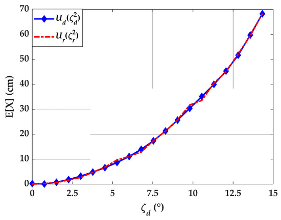
Figure 7.
Study on Tx’s orientation uncertainty based on the direct and reverse processes.
The expectation of the reverse process reveals some difficulties. The quadratic forms in the left side of (7) are invariant to rotations, which would imply that orientation uncertainties do not affect error performance. Since this is not the case, we approach the problem in a similar manner as in the case of Tx’s position uncertainties, that is, assuming that the effect of random headings can be reproduced by affecting the Tx’s positions with a random perturbation. Following this approach, the expectation of the reverse process can be cast as:
where and are the equivalent position perturbations, which are functions of the random orientation angles , , and . Equating and , allows to retrieve the correction values for the angle uncertainty, as a function of . To show that the processes are indeed equivalent, we performed the simulation for , the results are depicted in Figure 7. As it can be seen the two expectations match well and reveal that the effect of orientation uncertainty is worse than the position uncertainty.
3.3. Lighting Uniformity
In the indoor environments, it is essential to uniformly distribute inside the illuminated zone [27]. This constraint is generally assumed in well-lit spaces, where the uniformity of light is linked to the best perception of the objects. The uniform distribution of light in the room, , is represented as the ratio of the minimum to maximum power intensity at the receiving plane, which is given by:
Lighting uniformity relies on the three factors related to the Txs, i.e., the distance between the Txs, HPA, and the number of Txs. Figure 8 illustrates the lighting uniformity as a function of the number of Txs (i.e., 4 and 9) and for different values of HPA.
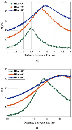
Figure 8.
Comparison of uniformity for different HPA and distance between the Txs in case of (a) 4-Tx, and (b) 9-Tx.
It is noticed from the figure that, a higher number of Txs provide improved uniformity. The maximum uniformity is achieved at distances of 3.4 and 2.6 m for HPA of 60° for 4- and 9-Tx, respectively. It is interesting to notice that, the same factors influence both lighting uniformity and positioning accuracy. It is usually believed that, positioning accuracy can be enhanced with higher uniformity. However, our study reveals that, this is not a general rule, moreover, HPA seems to have a more prominent impact on the positioning accuracy than the uniformity.
4. Simulation Results
In this section, the performance of the proposed VLP system is evaluated by simulation results. We consider the scenario where the LED-based Txs are located on the ceiling of a room of dimension 6 × 6 × 3 m3, which are assumed to be the same and modelled as pointwise Lambertian sources with order m depending ζ on the value of HPA, see (2). In practical environments also, the square LED placement layout is common. We have considered three different cases of 4-, 9-, and 16-LEDs, which are arranged in a square grid on the ceiling plane. The Rx is located on the ground plane. For all simulation purposes, the resolution of the grid is fixed at 1 cm, which implies that the PD can be placed at 3600 different locations. All the key parameters for the simulation are detailed in Table 2.
Table 2.
The key parameters for the indoor VLP system.
4.1. Positioning Error Dependence on Lighting Uniformity
This section analyses the influence of lighting uniformity and HPA on εp. Here, we vary the uniformity between 0.5 and 0.8 in steps of 0.05 and for HPA of 40° and 60°. For this, we first select the values of distance between the Txs according to the results of Figure 8. Following this, we estimate εp for each set of conditions using NLLS and the polynomial regression power-distance model. εp for different values of uniformity for 4-, 9-, and 16-Tx are illustrated in Figure 9. It is observed that the minimum εp is attained for the case of 4-Tx with HPA and uniformity of 60° and 0.65, respectively, whereas, in the case of 9-Tx, the minimum εp is achieved with HPA of 60° and uniformity equal to 0.55. For the 16-Tx case, the minimum εp is accomplished with an HPA of 40° and with the uniformity of 0.65. It is clear from Figure 9 that, (i) low to a moderate value of lighting uniformity can support low εp; and (ii) an optimal value for the number of Txs and the associated HPA, which do not match the optimal value of lighting uniformity conditions. Under the simulated conditions, the optimal values for the HPA, uniformity, and distance between the Tx based on the lowest εp are shown in Table 3.
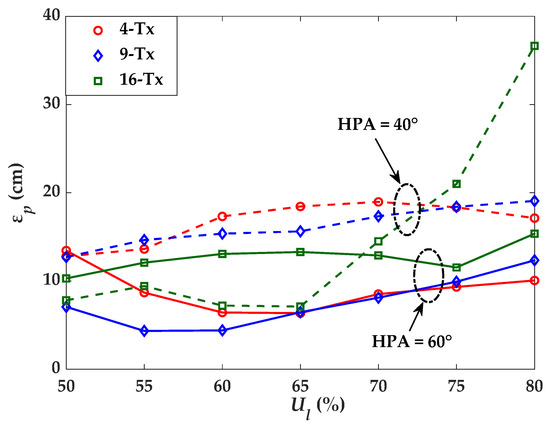
Figure 9.
Comparison of εp for different Txs and uniformity.
Table 3.
The optimized values for all cases of Txs.
4.2. Impact of Tx’s Position and Orientation Uncertainty on Error Performance
In this section, we investigate the impact of Tx’s position uncertainties σ and the Tx’s orientation uncertainties on the error performance. We follow the same approach that has been described in detail in Section 3.1. The simulation follows the reverse method with 1000 random iterations for each σ value using the adjusted variance values given by (16), where a random displacement vector () is added in the ideal Tx positions as explained in (11). The quantile function is employed as a performance metric considering both, its average and standard deviation, over the 1000 random iterations to obtain the confidence interval of εp, which is given by:
where is the percentage of the confidence interval.
Figure 10 illustrates the average and standard deviation of the 95% quantile of εp as a function of σ for 4-, 9-, and 16-Tx for the Tx’s positioning uncertainty. It is observed that the effect of Tx’s position uncertainty, σ, traduces in an increasing error dependence, which is more prominent for set-ups with a lower number of Txs. The standard deviation of the error quantile, i.e., the increasing error also confirms an increasing trend with σ, is more evident for the 4-Tx case. It is noticed that, for σ of 5 cm the average positioning errors are 23.3, 15.1, and 13.2 cm, with the standard deviation values of 6.4, 4.1, and 2.7 cm for 4-, 9-, and 16-Tx cases, respectively. Figure 10 suggests that the error dependence on the Tx’s position uncertainty can be lowered by increasing the number of Txs.
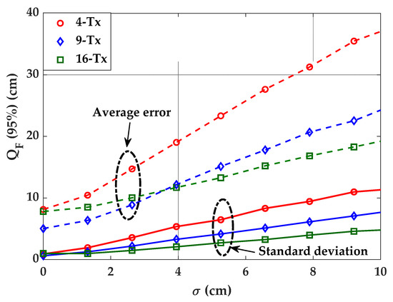
Figure 10.
Comparison of positioning error for different Txs and σ.
Figure 11 depicts the average and standard deviation of the 95% quantile of εp or as a function of for 4-, 9-, and 16-Tx for the Tx’s orientation uncertainty. It is clear from the figure that, alike the case of Tx’s position uncertainty, the effect has more significant error dependence for set-ups with a lower number of Txs. It is observed that for of 5°, the average positioning errors are 31.9, 20.6, and 17 cm, with the standard deviation values of 9.2, 6.3, and 3.9 cm for 4-, 9-, and 16-Tx cases, respectively. The increasing error also proves an increasing trend with , therefore, the placement of Tx with the accurate Tx’s position and its orientation should be taken into consideration, as the error may rise even with low values of set-up uncertainties.
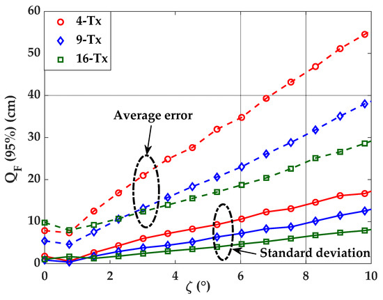
Figure 11.
Comparison of positioning error for different Txs and .
5. Conclusions
In this paper, we demonstrated the influence of Tx’s position and orientation uncertainty on the performance of VLP systems based on RSS. From the results, we can conclude that light uniformity and Tx’s HPA are crucial design parameters for developing an efficient VLP system. The selection of the Tx’s HPA as well as the optimum distance between Txs have to be carefully implemented. Moreover, we showed that the best uniformity and optimum error performance were not met for the same conditions, inferring necessary design trade-offs. Furthermore, the effect of error dependence on Tx’s position and orientation uncertainty reduced with increasing the number of Txs. In case of square grid Tx placement for a VLP system, the number of Txs can be further explored as an added variable to optimize both light uniformity and error performance, as it reduces the HPA for smaller distances between Txs.
Author Contributions
The contributions of the authors in this paper are the following: conceptualization: N.C. and L.N.A.; investigation: N.C.; methodology: N.C., L.N.A. and Z.G.; project administration: L.N.A. and Z.G.; software: N.C.; validation: L.N.A. and Z.G. All authors have read and agreed to the published version of the manuscript.
Funding
This research was funded by H2020/MSCA-ITN funding program under the framework of the European Training Network on Visible Light Based Interoperability and Networking, project (VisIoN) grant agreement no 764461.
Institutional Review Board Statement
Not applicable.
Informed Consent Statement
Not applicable.
Data Availability Statement
Not applicable.
Acknowledgments
This paper was raised under the frameworks of the COST Action NEWFOCUS (CA19111), supported by COST (European Cooperation in Science and Technology).
Conflicts of Interest
The authors declare no conflict of interest.
Nomenclature
| ADOA | Angle difference of arrival |
| ANN | Artificial neural network |
| AOA | Angle of arrival |
| CDF | Cumulative distribution function |
| FOV | Field of view |
| GPS | Global positioning system |
| HPA | Half power angle |
| IoT | Internet of things |
| IP | Indoor positioning |
| LEDs | Light-emitting diodes |
| LLS | Linear least square |
| LOS | Line of sight |
| NLLS | Nonlinear least square |
| NLOS | Non-line of sight |
| OOK | On-off keying |
| PD | Photodiode |
| Probability distribution function | |
| PR | Polynomial regression |
| RF | Radio frequency |
| RFID | Radio frequency identification |
| RSS | Received signal strength |
| Rx | Receiver |
| SNR | Signal-to-noise ratio |
| TDOA | Time difference of arrival |
| TOA | Time of arrival |
| Tx | Transmitter |
| UWB | Ultra-wide band |
| VLC | Visible light communication |
| VLP | Visible light positioning |
References
- Chaudhary, N.; Alves, L.N.; Ghassemblooy, Z. Current Trends on Visible Light Positioning Techniques. In Proceedings of the 2019 2nd West Asian Colloquium on Optical Wireless Communications (WACOWC), Tehran, Iran, 27–28 April 2019; pp. 100–105. [Google Scholar]
- Do, T.-H.; Yoo, M. An In-Depth Survey of Visible Light Communication Based Positioning Systems. Sensors 2016, 16, 678. [Google Scholar] [CrossRef] [PubMed]
- Yassin, A.; Nasser, Y.; Awad, M.; Al-Dubai, A.; Liu, R.; Yuen, C.; Raulefs, R.; Aboutanios, E. Recent Advances in Indoor Localization: A Survey on Theoretical Approaches and Applications. IEEE Commun. Surv. Tutor. 2017, 19, 1327–1346. [Google Scholar] [CrossRef]
- Gezici, S.; Tian, Z.; Giannakis, G.B.; Kobayashi, H.; Molisch, A.F.; Poor, H.V.; Sahinoglu, Z. Localization via Ultra-Wideband Radios: A Look at Positioning Aspects for Future Sensor Networks. IEEE Signal Process. Mag. 2005, 22, 70–84. [Google Scholar] [CrossRef]
- Tariq, Z.B.; Cheema, D.M.; Kamran, M.Z.; Naqvi, I.H. Non-GPS Positioning Systems: A Survey. ACM Comput. Surv. 2017, 50, 1–34. [Google Scholar] [CrossRef]
- Luo, J.; Fan, L.; Li, H. Indoor Positioning Systems Based on Visible Light Communication: State of the Art. IEEE Commun. Surv. Tutor. 2017, 19, 2871–2893. [Google Scholar] [CrossRef]
- Armstrong, J.; Sekercioglu, Y.; Neild, A. Visible Light Positioning: A Roadmap for International Standardization. IEEE Commun. Mag. 2013, 51, 68–73. [Google Scholar] [CrossRef]
- Zhuang, Y.; Wang, Q.; Shi, M.; Cao, P.; Qi, L.; Yang, J. Low-Power Centimeter-Level Localization for Indoor Mobile Robots Based on Ensemble Kalman Smoother Using Received Signal Strength. IEEE Internet Things J. 2019, 6, 6513–6522. [Google Scholar] [CrossRef]
- Zhu, B.; Cheng, J.; Wang, Y.; Yan, J.; Wang, J. Three-Dimensional VLC Positioning Based on Angle Difference of Arrival With Arbitrary Tilting Angle of Receiver. IEEE J. Sel. Areas Commun. 2018, 36, 8–22. [Google Scholar] [CrossRef]
- Xu, J.; Gong, C.; Xu, Z. Experimental Indoor Visible Light Positioning Systems With Centimeter Accuracy Based on a Commercial Smartphone Camera. IEEE Photonics J. 2018, 10, 1–17. [Google Scholar] [CrossRef]
- Naeem, A.; Hassan, N.U.; Pasha, M.A.; Yuen, C.; Sikora, A. Performance Analysis of TDOA-Based Indoor Positioning Systems Using Visible LED Lights. In Proceedings of the 2018 IEEE 4th International Symposium on Wireless Systems within the International Conferences on Intelligent Data Acquisition and Advanced Computing Systems (IDAACS-SWS), Lviv, Ukraine, 20–21 September 2018; pp. 103–107. [Google Scholar]
- Xie, C.; Guan, W.; Wu, Y.; Fang, L.; Cai, Y. The LED-ID Detection and Recognition Method Based on Visible Light Positioning Using Proximity Method. IEEE Photonics J. 2018, 10, 1–16. [Google Scholar] [CrossRef]
- Plets, D.; Bastiaens, S.; Stevens, N.; Martens, L.; Joseph, W. Monte-Carlo Simulation of the Impact of LED Power Uncertainty on Visible Light Positioning Accuracy. In Proceedings of the 2018 11th International Symposium on Communication Systems, Networks & Digital Signal Processing (CSNDSP), Budapest, Hungary, 18–20 July 2018; pp. 1–6. [Google Scholar]
- Gu, W.; Aminikashani, M.; Deng, P.; Kavehrad, M. Impact of Multipath Reflections on the Performance of Indoor Visible Light Positioning Systems. J. Light. Technol. 2016, 34, 2578–2587. [Google Scholar] [CrossRef]
- Mousa, F.I.K.; Almaadeed, N.; Busawon, K.; Bouridane, A.; Binns, R.; Elliot, I. Indoor Visible Light Communication Localization System Utilizing Received Signal Strength Indication Technique and Trilateration Method. Opt. Eng. 2018, 57, 1. [Google Scholar] [CrossRef]
- Wang, X.; Shen, J. Machine Learning and Its Applications in Visible Light Communication Based Indoor Positioning. In Proceedings of the 2019 International Conference on High Performance Big Data and Intelligent Systems (HPBD&IS), Shenzhen, China, 9–11 May 2019; pp. 274–277. [Google Scholar]
- Shawky, S.; El-Shimy, M.A.; El-Sahn, Z.A.; Rizk, M.R.M.; Aly, M.H. Improved VLC-Based Indoor Positioning System Using a Regression Approach with Conventional RSS Techniques. In Proceedings of the 2017 13th International Wireless Communications and Mobile Computing Conference (IWCMC), Valencia, Spain, 26–30 June 2017; pp. 904–909. [Google Scholar]
- Plets, D.; Bastiaens, S.; Martens, L.; Joseph, W. An Analysis of the Impact of LED Tilt on Visible Light Positioning Accuracy. Electronics 2019, 8, 389. [Google Scholar] [CrossRef]
- Plets, D.; Bastiaens, S.; Martens, L.; Joseph, W. Performance Assessment of Artificial Neural Networks on the RSS-Based Visible Light Positioning Accuracy with Random Transmitter Tilt. In Proceedings of the CSNDSP, Porto, Portugal, 20–22 July 2020; Volume 8, p. 389. [Google Scholar]
- Chaudhary, N.; Alves, L.N.; Ghassemlooy, Z. Impact of Transmitter Positioning Uncertainty on RSS-Based Visible Light Positioning Accuracy. In Proceedings of the 2020 12th International Symposium on Communication Systems, Networks and Digital Signal Processing (CSNDSP), Porto, Portugal, 20 July 2020; pp. 1–6. [Google Scholar]
- Shi, G.; Li, Y.; Cheng, W. Accuracy Analysis of Indoor Visible Light Communication Localization System Based on Received Signal Strength in Non-Line-of-Sight Environments by Using Least Squares Method. Opt. Eng. 2019, 58, 1. [Google Scholar] [CrossRef]
- Ghassemblooy, Z.; Popoola, W.; Rajbhandari, S. Optical Wireless Communications: System and Channel Modelling with Matlab®; CRC Press: Boca Raton, FL, USA, 2019. [Google Scholar]
- Chaudhary, N.; Alves, L.N.; Ghassemblooy, Z. Feasibility Study of Reverse Trilateration Strategy with a Single Tx for VLP. In Proceedings of the 2019 2nd West Asian Colloquium on Optical Wireless Communications (WACOWC), Tehran, Iran, 27–28 April 2019; pp. 121–126. [Google Scholar]
- Sun, X.; Duan, J.; Zou, Y.; Shi, A. Impact of Multipath Effects on Theoretical Accuracy of TOA-Based Indoor VLC Positioning System. OSA Publishing: Washington, DC, USA, 2015; Volume 4. [Google Scholar]
- Chaudhary, N.; Younus, O.I.; Alves, L.N.; Ghassemlooy, Z.; Zvanovec, S.; Le-Minh, H. An Indoor Visible Light Positioning System Using Tilted LEDs with High Accuracy. Sensors 2021, 21, 920. [Google Scholar] [CrossRef] [PubMed]
- Shiquan, W. Computation of a Trust Region Step. ACTA Math. Appl. Sin. 1991, 7, 354–362. [Google Scholar]
- Hu, Y.; Luo, M.R.; Yang, Y. A Study on Lighting Uniformity for LED Smart Lighting System. In Proceedings of the 2015 12th China International Forum on Solid State Lighting (SSLCHINA), Shenzhen, China, 2–4 November 2015; pp. 127–130. [Google Scholar]


Publisher’s Note: MDPI stays neutral with regard to jurisdictional claims in published maps and institutional affiliations. |
© 2021 by the authors. Licensee MDPI, Basel, Switzerland. This article is an open access article distributed under the terms and conditions of the Creative Commons Attribution (CC BY) license (https://creativecommons.org/licenses/by/4.0/).