
Double-Scale Adaptive Transmission in Time-Varying Channel for Underwater Acoustic Sensor Networks


Abstract
1. Introduction
- To improve the energy efficiency and reliability of data transmission, we propose a double-scale adaptive transmission mechanism for UASNs. Specifically, the historical channel state series is used for channel state prediction, and then the transmission mode is determined adaptively.
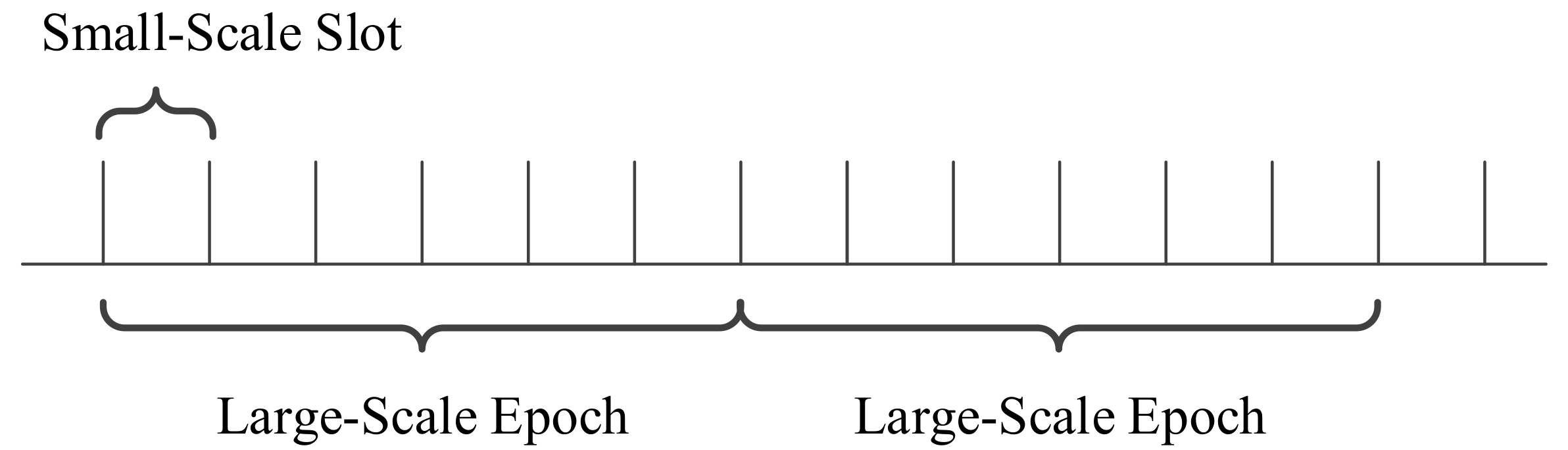
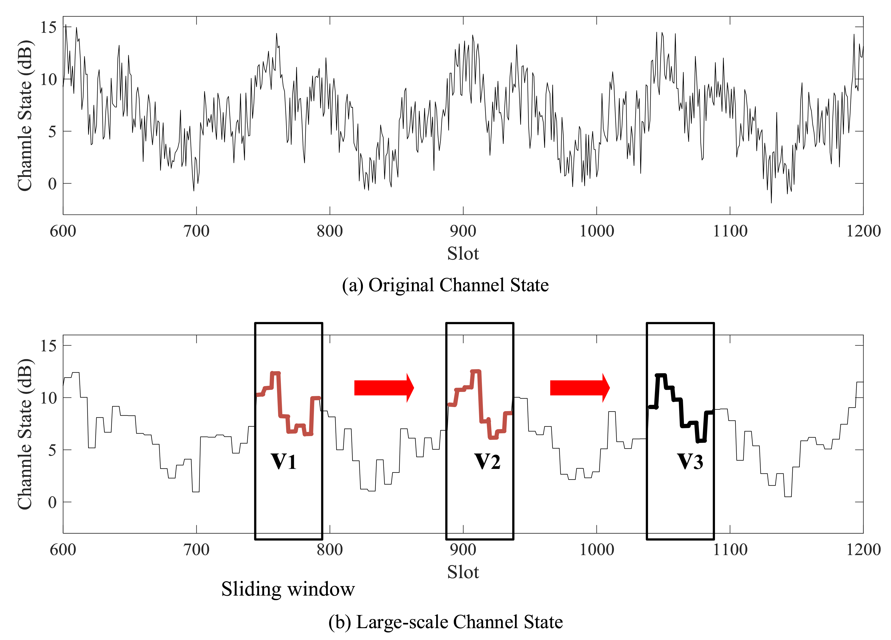
- To balance the accuracy and computational complexity of channel states prediction, we propose to decompose the channel state series with two different time scales. For the large-scale channel state, a k-nearest neighbor algorithm with sliding window is designed to predict the fluctuation tendency, and then a small-scale channel state prediction algorithm is developed to enhance the accuracy.
- To determine the specific configuration of data communication in UASNs, we design an energy-efficient transmission algorithm. In particular, the long-term modulation and coding problem is formulated and optimized with the constraint of limited energy cost.
2. Related Works
2.1. Channel State Prediction
2.2. Adaptive Data Transmission
3. Double-Scale Adaptive Transmission Mechanism for UASNs
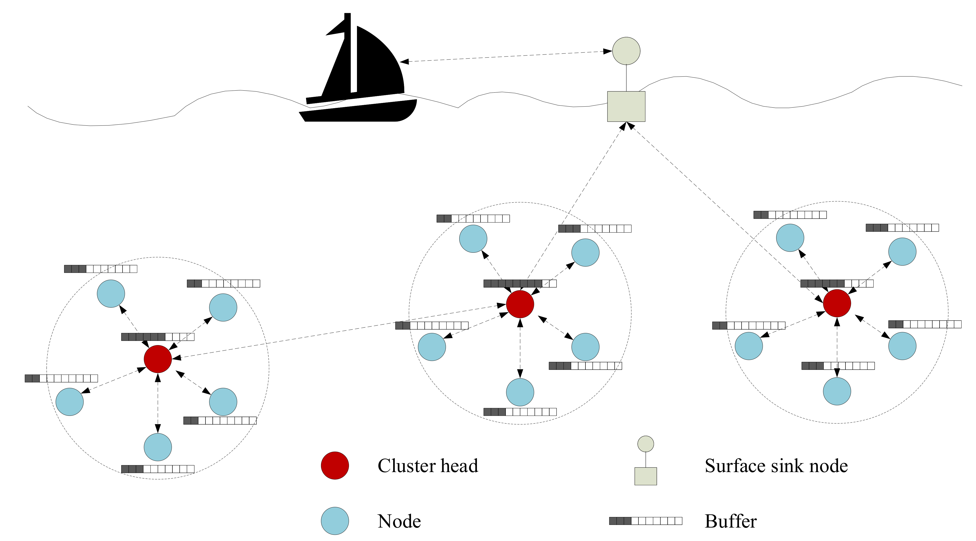
3.1. System Model
3.2. Underwater Acoustic Channel Model
3.3. Adaptive Transmission Framework
4. Double-Scale Channel State Prediction
4.1. Large-Scale Channel State Prediction
4.1.1. k-Nearest Neighbor Prediction Algorithm with Sliding Window
| Algorithm 1: large-scale channel state prediction |
| Input: training set , test vector Output: predicted large-scale channel state
|
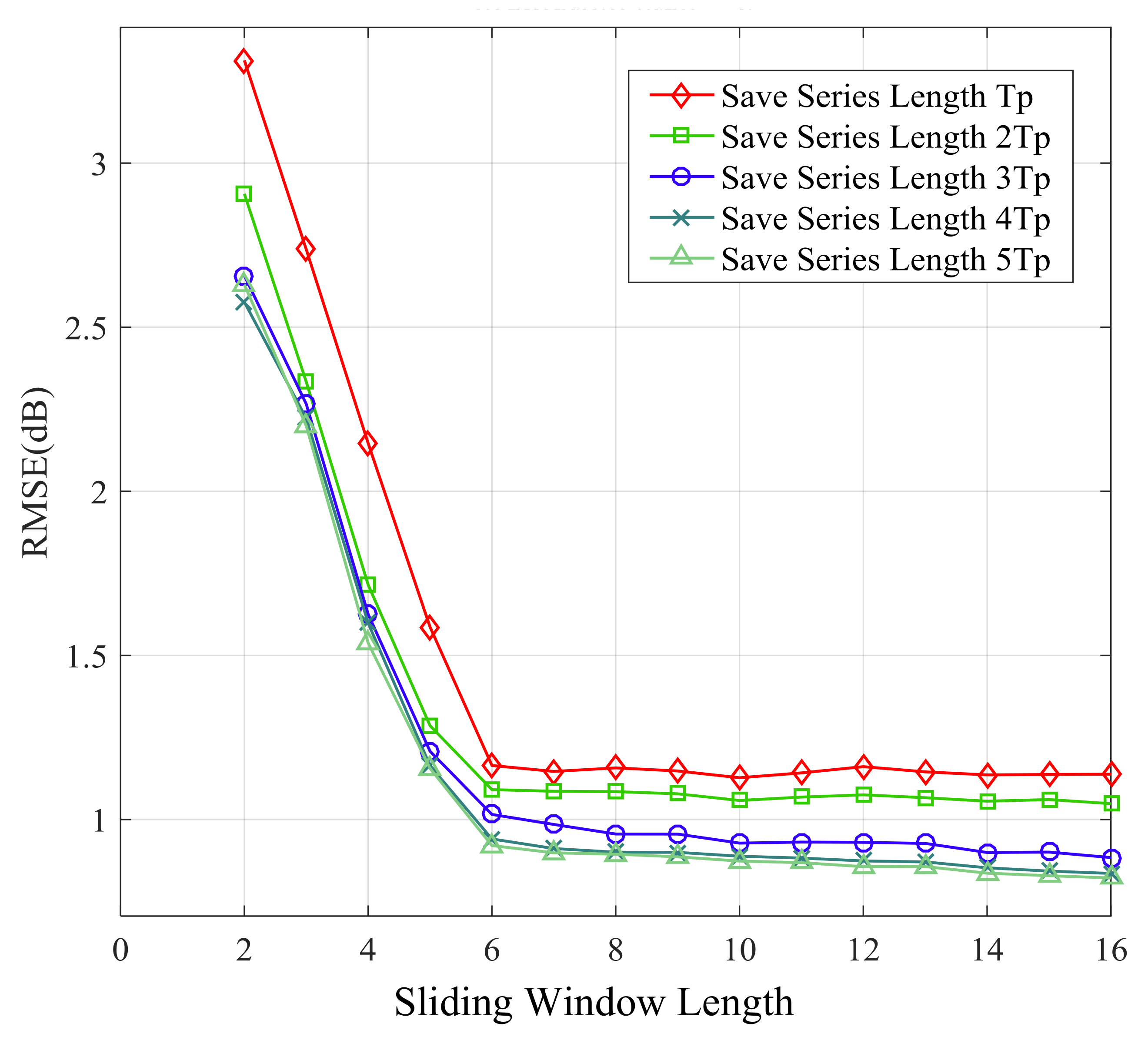
4.1.2. Calculation of Stored Series Length
4.2. Small-Scale Channel State Prediction
4.2.1. Small-Scale Channel Fluctuating Features
4.2.2. Residual Series Prediction
5. Energy-Efficient Transmission Algorithm
5.1. Problem Formulation
- (1)
- When the bits arrival rate is less than the maximum transmission capacity, and the buffer size is less than the buffer threshold, the amount of successfully transmitted bits should be more than the expected arrival bits.
- (2)
- When the bits arrival rate is less than the maximum transmission capacity, and the buffer size is greater than the buffer threshold, the amount of successfully transmitted bits should be more than the expected arrival bits plus a certain proportion of the buffer length, .
- (3)
- When the bits arrival rate is greater than the maximum transmission capacity, the message should be sent according to the maximum transmission capacity.
5.2. Modulation Coding Method Selection
| Algorithm 2: Modulation and coding mode scheduling |
| Input: predicted large-scale channel state, buffer state, data arrival rate Output: modulation and coding modes
|
6. Performance Analysis and Computational Complexity
6.1. Performance Analysis
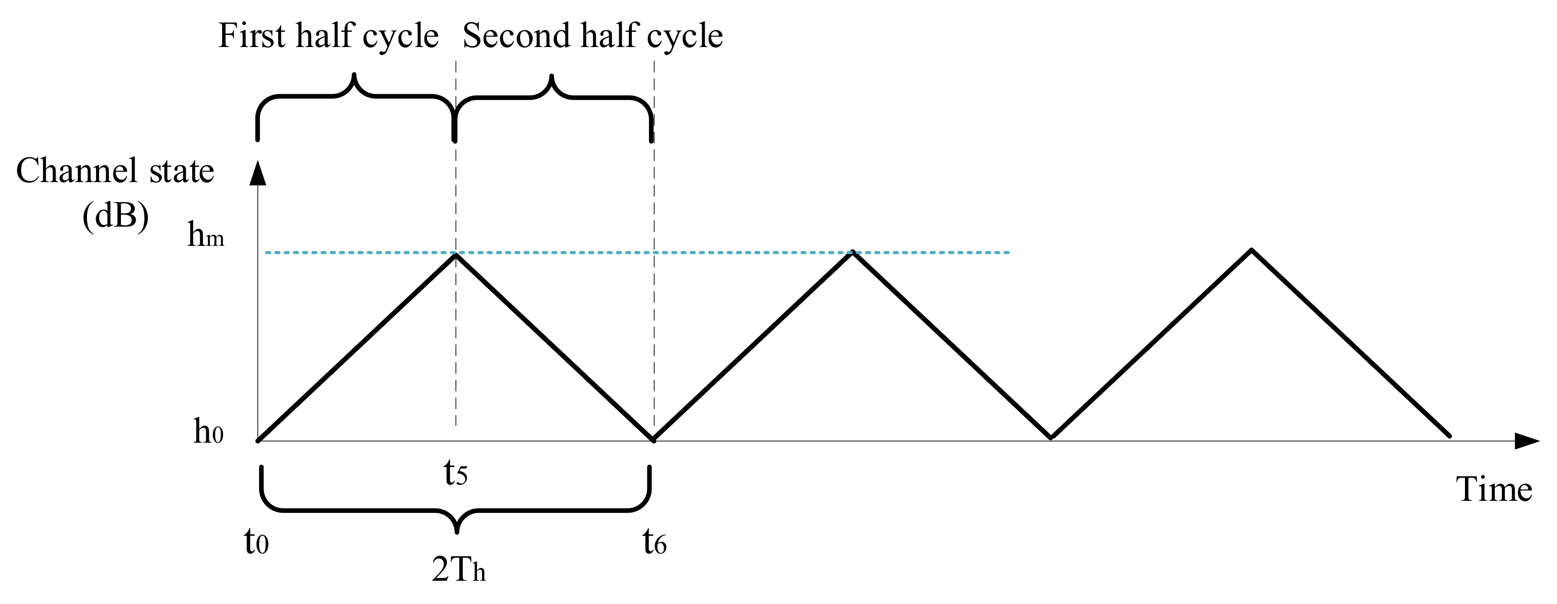
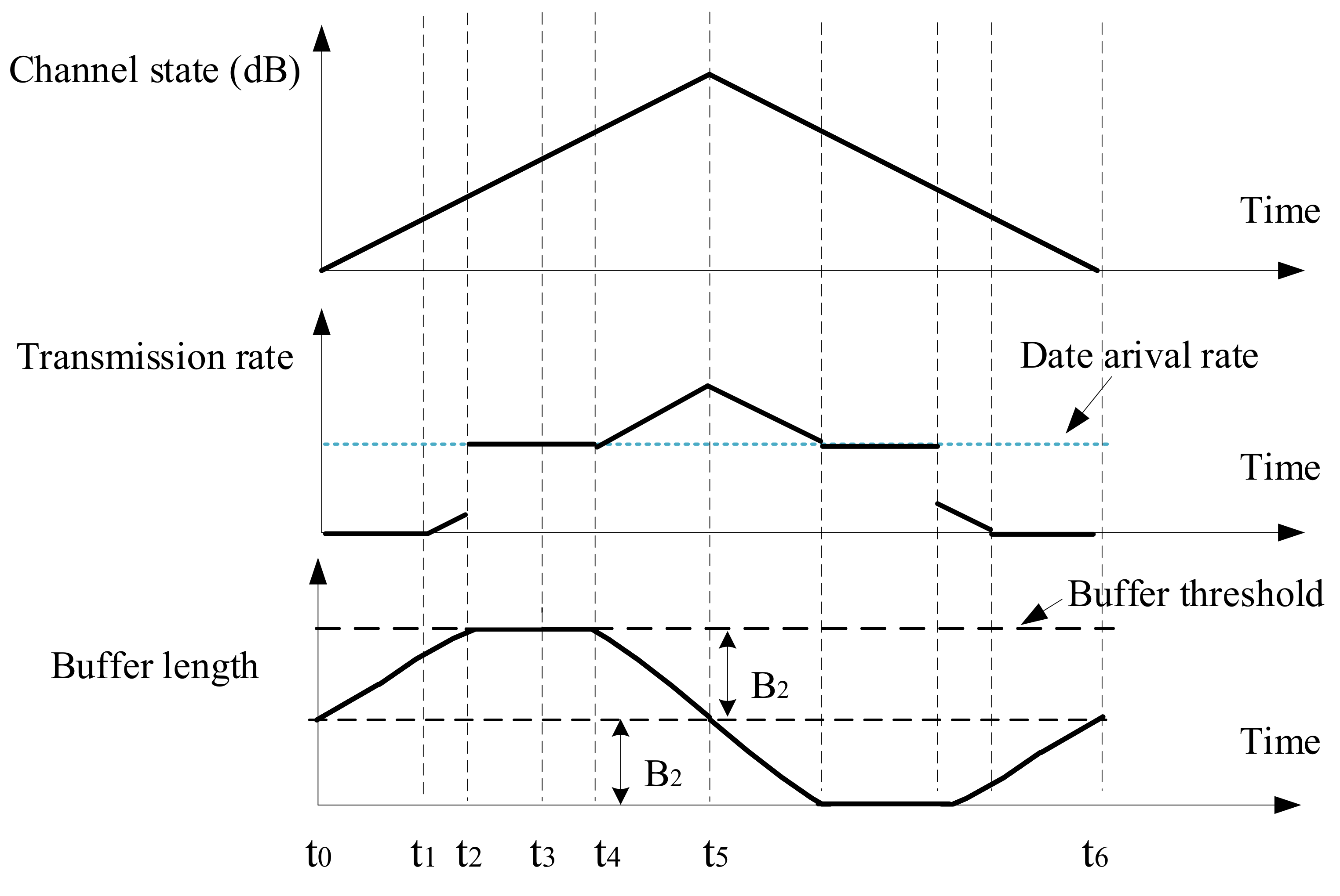
6.1.1. Special Channel State Series
6.1.2. Energy Cost Minimization Problem
6.1.3. Reasonable Buffer Threshold
6.1.4. Performance with Large Buffer Threshold
6.1.5. Performance with Small Buffer Threshold
6.2. Computational Complexity
7. Performance Evaluation
7.1. Simulation Setting
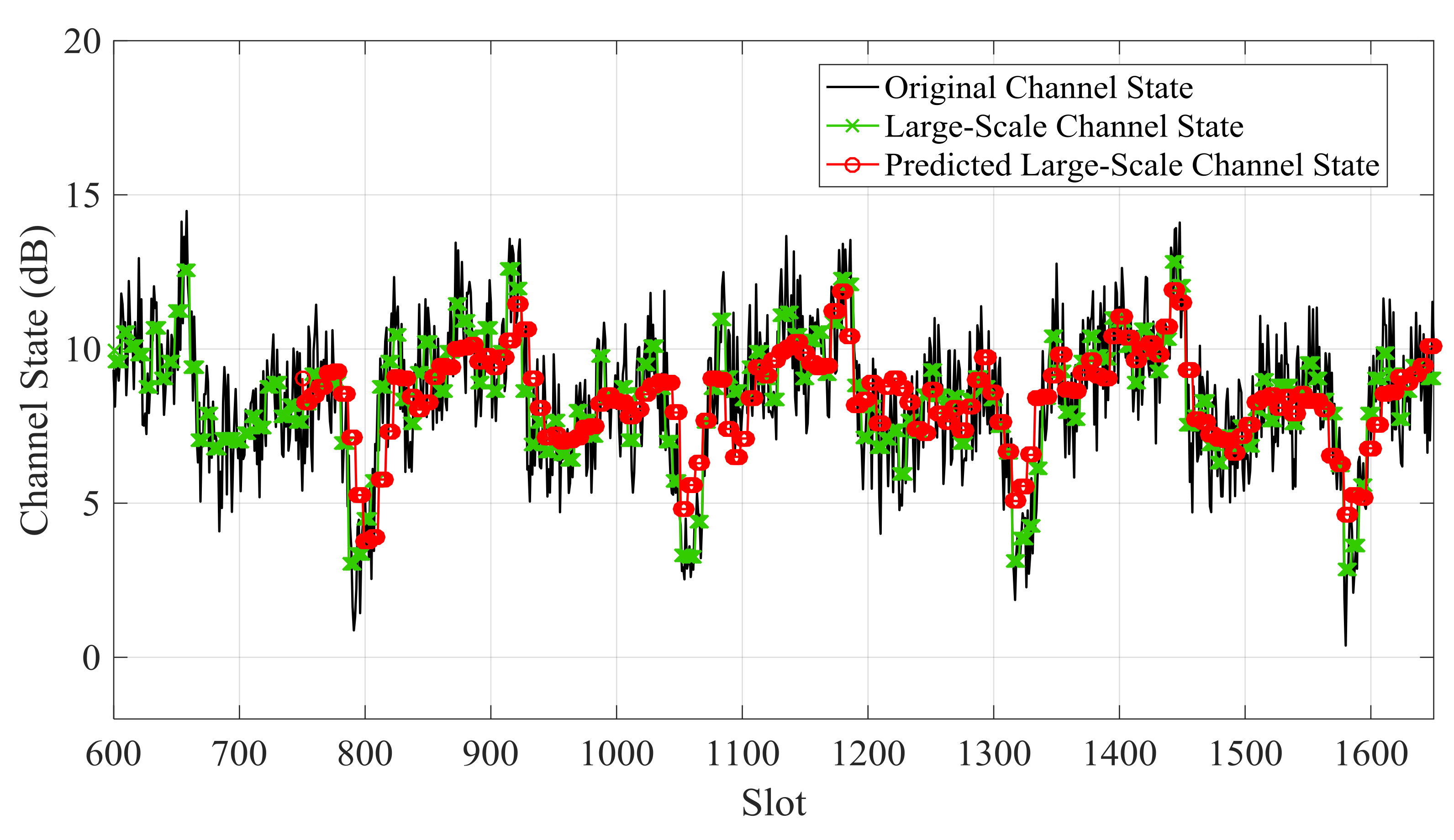
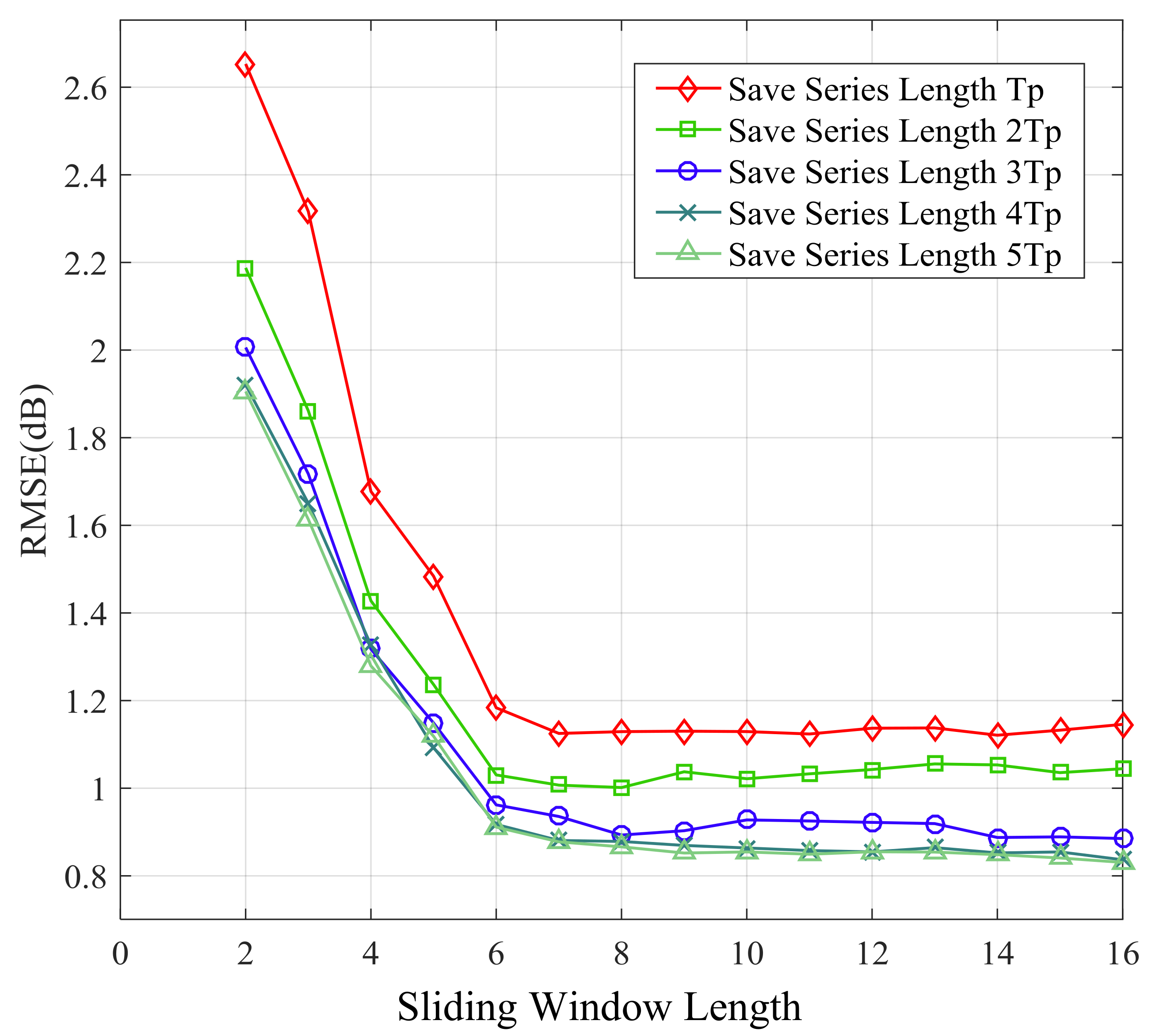
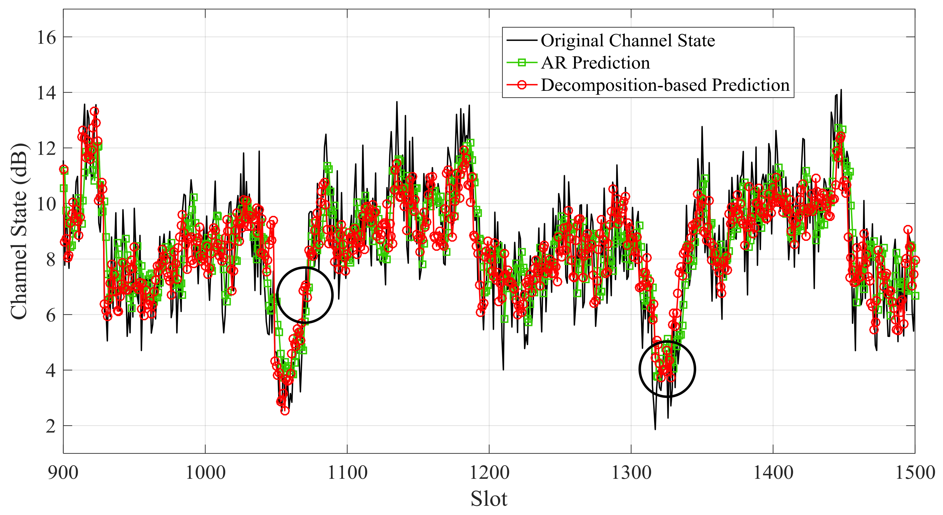
7.2. Channel Prediction Performance
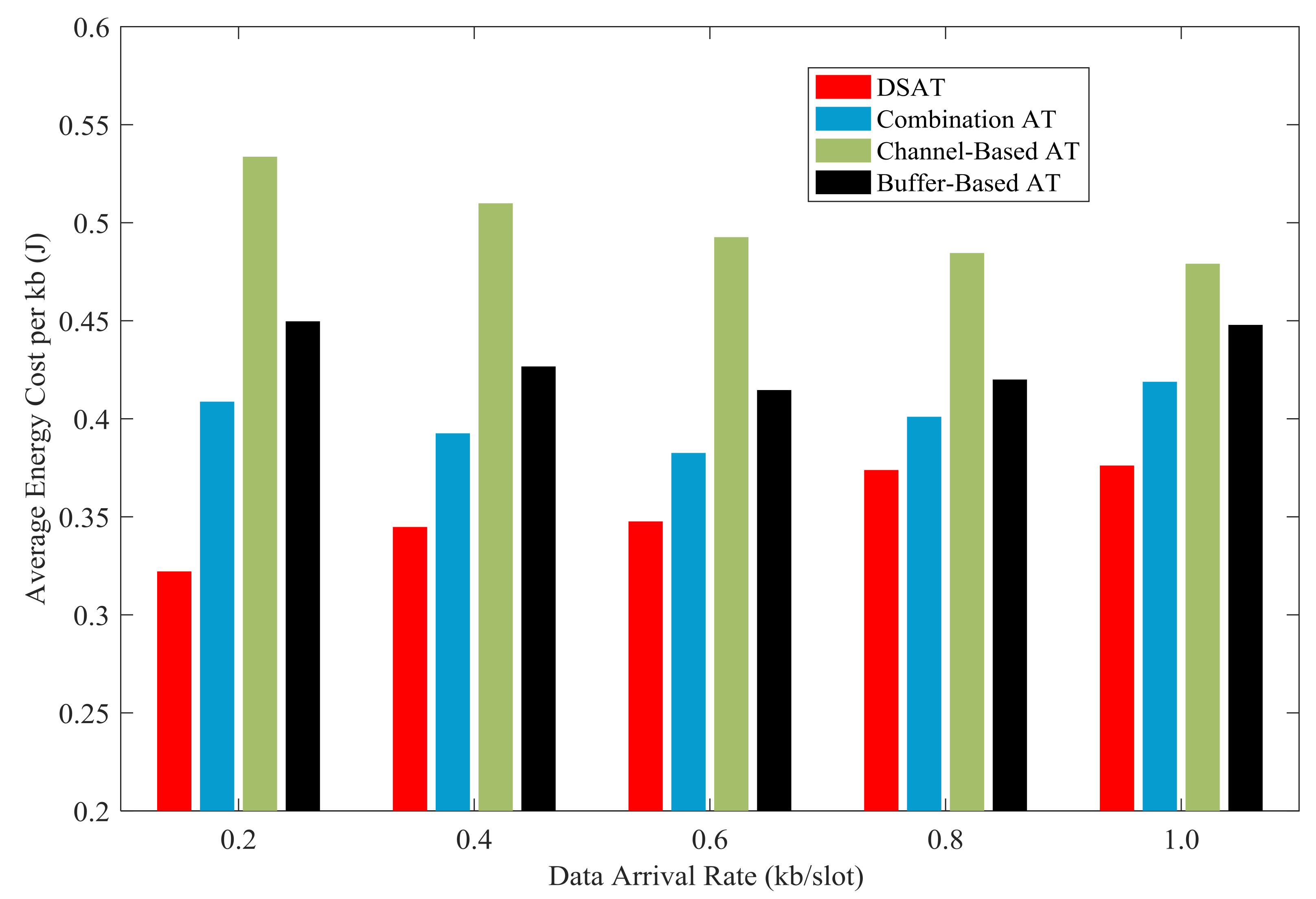
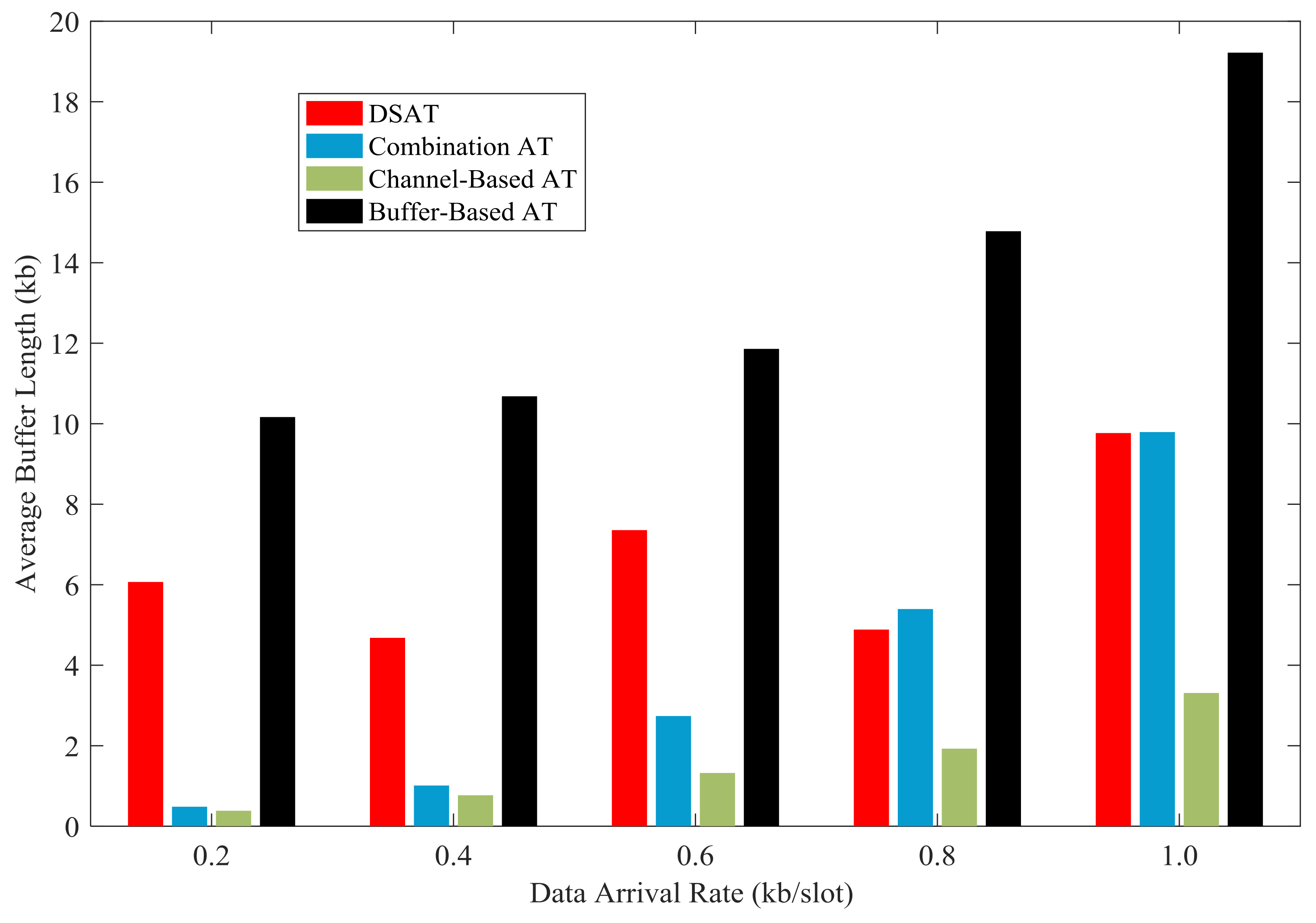
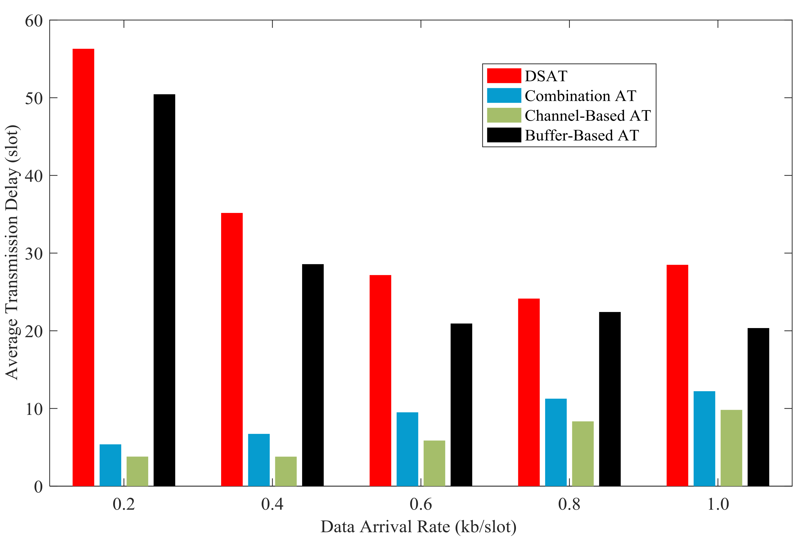
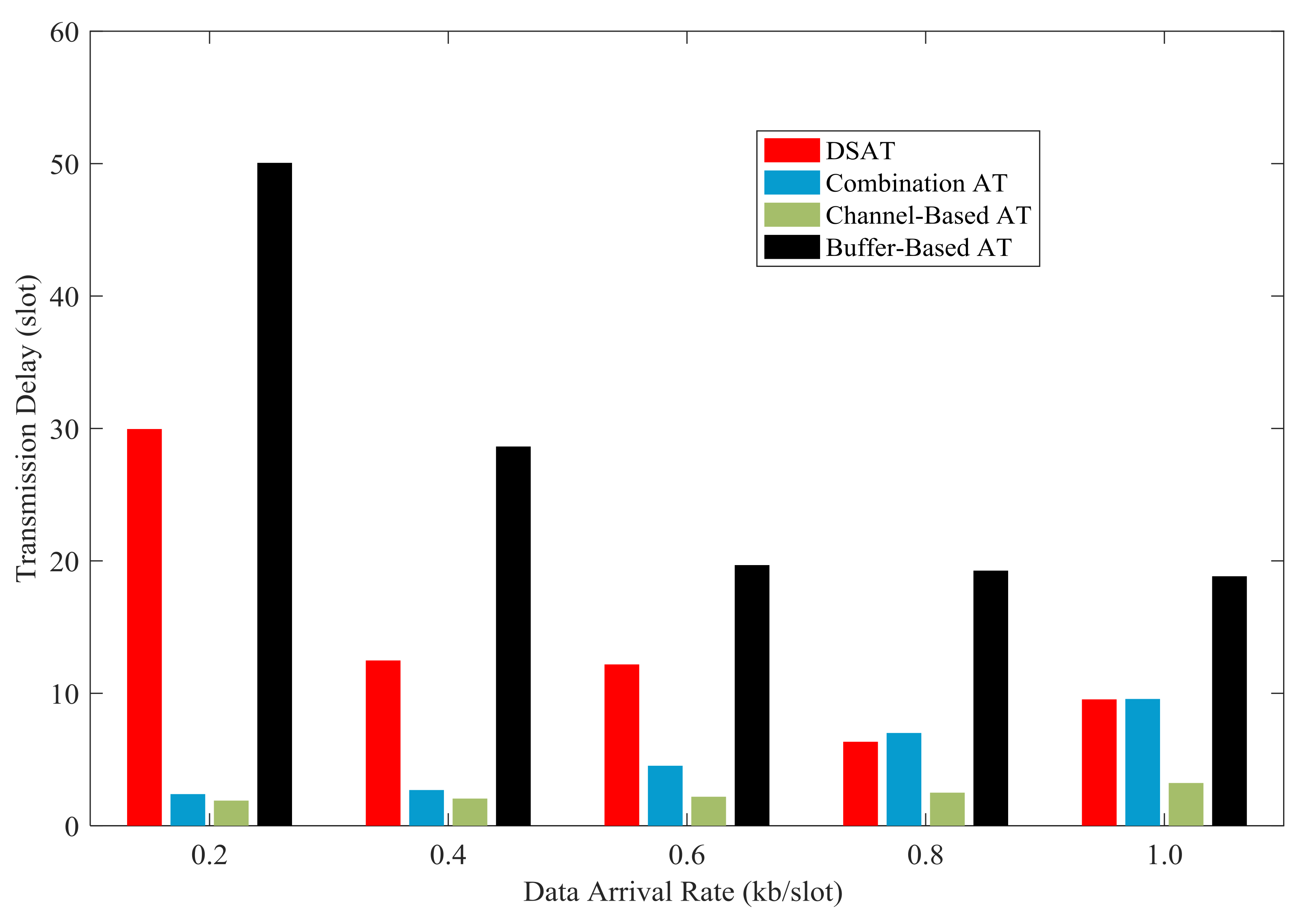
7.3. Data Transmission Performance Comparison
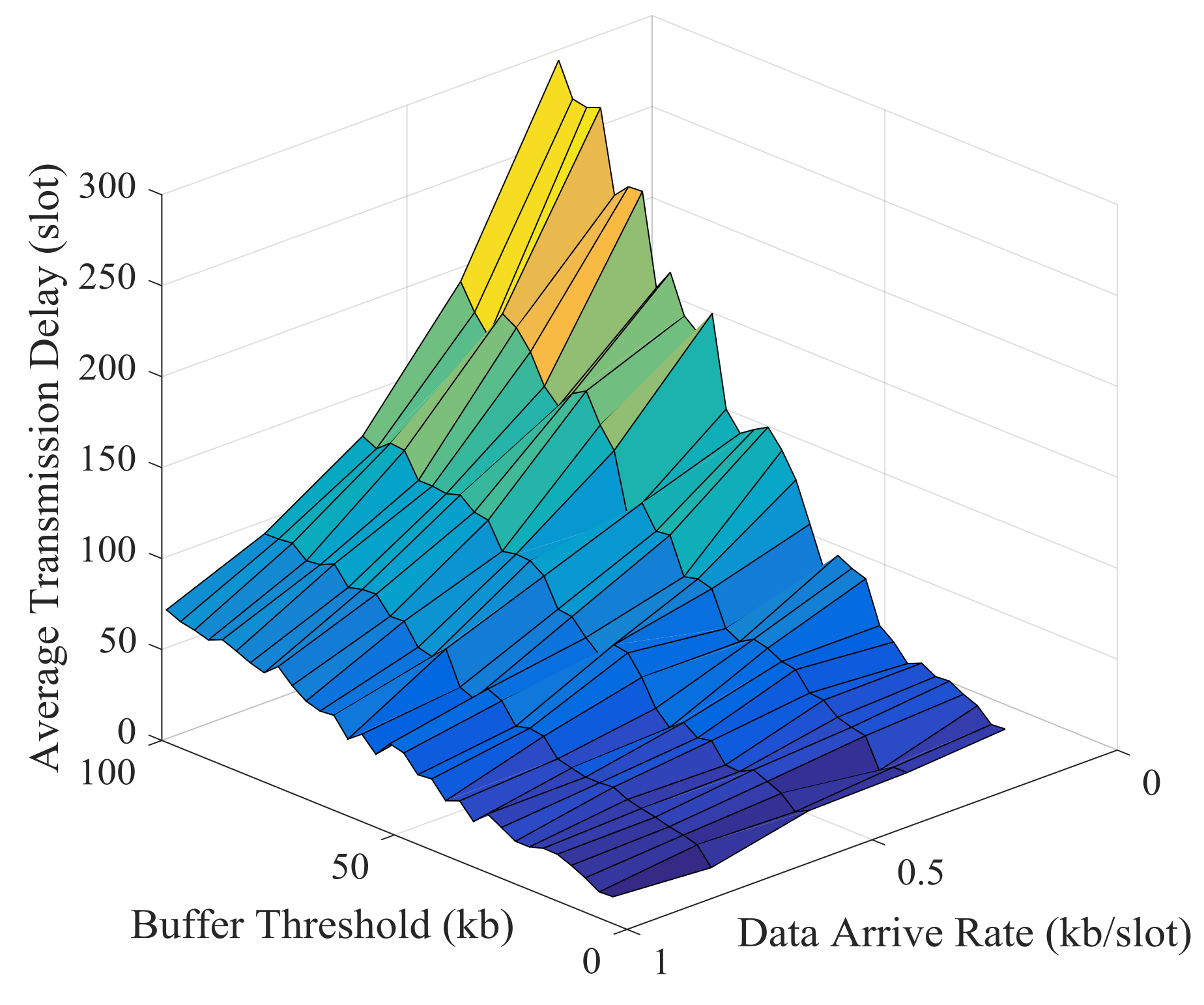
7.4. Influence of Buffer Threshold
8. Conclusions
Author Contributions
Funding
Institutional Review Board Statement
Informed Consent Statement
Data Availability Statement
Conflicts of Interest
References
- Wan, L.; Zhou, H.; Xu, X.; Huang, Y.; Zhou, S.; Shi, Z.; Cui, J.-H. Adaptive Modulation and Coding for Underwater Acoustic OFDM. IEEE J. Ocean. Eng. 2015, 40, 327–336. [Google Scholar] [CrossRef]
- Wang, H.; Wang, S.L.; Zhang, E.Y.; Lu, L.X. An Energy Balanced and Lifetime Extended Routing Protocol for Underwater Sensor Networks. Sensors 2018, 18, 1596. [Google Scholar] [CrossRef]
- Wei, X.H.; Guo, H.; Wang, X.W.; Wang, X.N.; Wang, C.; Guizani, M.; Du, X.J. A Co-Design-Based Reliable Low-Latency and Energy-Efficient Transmission Protocol for UWSNs. Sensors 2020, 20, 6370. [Google Scholar] [CrossRef] [PubMed]
- Han, S.; Li, L.; Li, X.B. Deep Q-Network-Based Cooperative Transmission Joint Strategy Optimization Algorithm for Energy Harvesting-Powered Underwater Acoustic Sensor Networks. Sensors 2020, 20, 6519. [Google Scholar] [CrossRef]
- Sun, W.S.; Wang, Z.H. Modeling and Prediction of Large-Scale Temporal Variation in Underwater Acoustic Channels. In Proceedings of the OCEANS Conference 2016, Shanghai, China, 10–13 April 2016; pp. 1–6. [Google Scholar]
- Merchant, N.D.; Brookes, K.L.; Faulkner, R.C.; Bicknell, A.W.J.; Godley, B.J.; Witt, M.J.J.S.R. Underwater Noise Levels in UK Waters. Sci. Rep. 2016, 6, 36942. [Google Scholar] [CrossRef]
- van Walree, P.A. Propagation and Scattering Effects in Underwater Acoustic Communication Channels. IEEE J. Ocean. Eng. 2013, 38, 614–631. [Google Scholar] [CrossRef]
- Huang, W.; Li, D.; Jiang, P. Underwater sound speed inversion by joint artificial neural network and ray theory. In Proceedings of the 13th International Conference on Underwater Networks & Systems, Shenzhen, China, 3–5 December 2018. [Google Scholar]
- Sun, W.S.; Wang, Z.H.; Jamalabdollahi, M.; Zekavat, S.A. Experimental Study on the Difference between Acoustic Communication Channels in Freshwater Rivers/Lakes and in Oceans. In Proceedings of the IEEE 48nd Asilomar Conference on Signals, Pacific Grove, CA, USA, 2–5 November 2014; pp. 333–337. [Google Scholar]
- El-Banna, A.A.A.; Wu, K.; ElHalawany, B.M. Opportunistic Cooperative Transmission for Underwater Communication Based on the Water’s Key Physical Variables. IEEE Sens. J. 2020, 20, 2792–2802. [Google Scholar] [CrossRef]
- Kuai, X.Y.; Sun, H.X.; Qi, J.; Cheng, E.; Xu, X.K.; Guo, Y.H.; Chen, Y.G. CSI Feedback-Based CS for Underwater Acoustic Adaptive Modulation OFDM System with Channel Prediction. China Ocean Eng. 2014, 28, 391–400. [Google Scholar] [CrossRef]
- Huda, M.; Putri, N.B.; Santoso, T.B. OFDM System with Adaptive Modulation for Shallow Water Acoustic Channel Environment. In Proceedings of the 6th IEEE International Conference on Communication, Semarang, Indonesia, 5–7 October 2017; pp. 55–58. [Google Scholar]
- Tomasi, B.; Preisig, J.C. Energy-Efficient Transmission Strategies for Delay Constrained Traffic with Limited Feedback. IEEE Trans. Wirel. Commun. 2015, 14, 1369–1379. [Google Scholar] [CrossRef]
- Jing, L.Y.; He, C.B.; Huang, J.G.; Ding, Z. Energy Management and Power Allocation for Underwater Acoustic Sensor Network. IEEE Sens. J. 2017, 17, 6451–6462. [Google Scholar] [CrossRef]
- Wang, C.; Wang, Z.; Sun, W.; Fuhrmann, D.R. Reinforcement Learning-Based Adaptive Transmission in Time-Varying Underwater Acoustic Channels. IEEE Access 2018, 6, 2541–2558. [Google Scholar] [CrossRef]
- Su, W.; Lin, J.; Chen, K.; Xiao, L.; En, C. Reinforcement Learning-Based Adaptive Modulation and Coding for Efficient Underwater Communications. IEEE Access 2019, 7, 67539–67550. [Google Scholar] [CrossRef]
- Radosevic, A.; Ahmed, R.; Duman, T.M.; Proakis, J.G.; Stojanovic, M. Adaptive OFDM Modulation for Underwater Acoustic Communications: Design Considerations and Experimental Results. IEEE J. Ocean. Eng. 2014, 39, 357–370. [Google Scholar] [CrossRef]
- Wang, Z.; Wang, C.; Sun, W. Adaptive Transmission Scheduling in Time-Varying Underwater Acoustic Channels. In Proceedings of the OCEANS Conference 2015, Washington, DC, USA, 19–22 October 2015; pp. 1–6. [Google Scholar]
- Sharma, P.; Chandra, K. Prediction of State Transitions in Rayleigh Fading Channels. IEEE Trans. Veh. Technol. 2007, 56, 416–425. [Google Scholar] [CrossRef]
- Liu, L.; Feng, H.; Yang, T.; Hu, B. MIMO-OFDM Wireless Channel Prediction by Exploiting Spatial-Temporal Correlation. IEEE Trans. Wirel. Commun. 2014, 13, 310–319. [Google Scholar] [CrossRef]
- Heidari, A.; Khandani, A.K.; McAvoy, D. Adaptive modelling and long-range prediction of mobile fading channels. IET Commun. 2010, 4, 39–50. [Google Scholar] [CrossRef]
- Schmidt, J.F.; Cousseau, J.E.; Wichman, R.; Werner, S. Low-Complexity Channel Prediction Using Approximated Recursive DCT. IEEE Trans. Circuits Syst. I Regul. Pap. 2011, 58, 2520–2530. [Google Scholar] [CrossRef]
- Bharamagoudra, M.R.; Manvi, S.S.; Gonen, B. Event Driven Energy Depth and Channel Aware Routing for Underwater Acoustic Sensor Networks: Agent Oriented Clustering Based Approach. Comput. Electr. Eng. 2017, 58, 1–19. [Google Scholar] [CrossRef]
- Basagni, S.; Petrioli, C.; Petroccia, R.; Spaccini, D. CARP: A Channel-Aware Routing Protocol for Underwater Acoustic Wireless Networks. Ad Hoc Netw. 2015, 34, 92–104. [Google Scholar] [CrossRef]
- Zhang, Y.; Venkatesan, R.; Dobre, O.A.; Li, C. Efficient Estimation and Prediction for Sparse Time-Varying Underwater Acoustic Channels. IEEE J. Ocean. Eng. 2020, 45, 1112–1125. [Google Scholar] [CrossRef]
- Zhao, X.N.; Hou, C.P.; Wang, Q. A New SVM-Based Modeling Method of Cabin Path Loss Prediction. Int. J. Antennas Propag. 2013, 2013, 1–7. [Google Scholar] [CrossRef]
- Zhao, Y.S.; Gao, H.; Beaulieu, N.C.; Chen, Z.H.; Ji, H. Echo State Network for Fast Channel Prediction in Ricean Fading Scenarios. IEEE Commun. Lett. 2017, 21, 672–675. [Google Scholar] [CrossRef]
- Tripathi, S.; De, S. Channel-Adaptive Transmission Protocols for Smart Grid IoT Communication. IEEE Internet Things J. 2020, 7, 7823–7835. [Google Scholar] [CrossRef]
- Joo, J.; Park, M.C.; Han, D.S.; Pejovic, V. Deep Learning-Based Channel Prediction in Realistic Vehicular Communications. IEEE Access 2019, 7, 27846–27858. [Google Scholar] [CrossRef]
- Diao, B.Y.; Xu, Y.J.; Li, C.; An, Z.L.; Wang, Q.; Chen, Z. A Nearest Neighbor Regression based Channel Estimation Algorithm for Acoustic Channel-Aware Routing. In Proceedings of the OCEANS Conference 2018, Shanghai, China, 28–31 May 2018; pp. 1–7. [Google Scholar]
- Long, X.B.; Sikdar, B. A Wavelet Based Long Range Signal Strength Prediction in Wireless Networks. In Proceedings of the 2008 IEEE International Conference on Communications, Beijing, China, 19–23 May 2008; pp. 2043–2047. [Google Scholar]
- Mi, X.; Liu, H.; Li, Y. Wind Speed Prediction Model Using Singular Spectrum Analysis, Empirical Mode Decomposition and Convolutional Support Vector Machine. Energy Conv. Manag. 2019, 180, 196–205. [Google Scholar] [CrossRef]
- Yu, L.; Wang, S.; Lai, K.K. Forecasting Crude Oil Price with an EMD-Based Neural Network Ensemble Learning Paradigm. Energy Econ. 2008, 30, 2623–2635. [Google Scholar] [CrossRef]
- Chen, C.-F.; Lai, M.-C.; Yeh, C.-C. Forecasting tourism demand based on empirical mode decomposition and neural network. Knowl. Based Syst. 2012, 26, 281–287. [Google Scholar] [CrossRef]
- Huang, W.L.; Letaief, K.B. Cross-Layer Scheduling and Power Control Combined with Adaptive Modulation for Wireless Ad Hoc Networks. IEEE Trans. Commun. 2007, 55, 728–739. [Google Scholar] [CrossRef]
- Zhu, J.; Song, Y.; Jiang, D.; Song, H. A New Deep-Q-Learning-Based Transmission Scheduling Mechanism for the Cognitive Internet of Things. IEEE Internet Things J. 2018, 5, 2375–2385. [Google Scholar] [CrossRef]
- Li, M.; Zhao, X.; Liang, H.; Hu, F. Deep Reinforcement Learning Optimal Transmission Policy for Communication Systems with Energy Harvesting and Adaptive MQAM. IEEE Trans. Veh. Technol. 2019, 68, 5782–5793. [Google Scholar] [CrossRef]
- An, K.; Liang, T. Hybrid Satellite-Terrestrial Relay Networks with Adaptive Transmission. IEEE Trans. Veh. Technol. 2019, 68, 12448–12452. [Google Scholar] [CrossRef]
- Ekerete, K.-M.; Awoseyila, A.; Evans, B. Robust Adaptive Margin for ACM in Satellite Links at EHF Bands. IEEE Commun. Lett. 2020, 24, 169–172. [Google Scholar] [CrossRef]
- Gu, S.; Jiao, J.; Huang, Z.; Wu, S.; Zhang, Q. ARMA-Based Adaptive Coding Transmission Over Millimeter-Wave Channel for Integrated Satellite-Terrestrial Networks. IEEE Access 2018, 6, 21635–21645. [Google Scholar] [CrossRef]
- Xiao, L.; Jiang, D.; Chen, Y.; Su, W.; Tang, Y. Reinforcement-Learning-Based Relay Mobility and Power Allocation for Underwater Sensor Networks Against Jamming. IEEE J. Ocean. Eng. 2020, 45, 1148–1156. [Google Scholar] [CrossRef]
- Valerio, V.D.; Petrioli, C.; Pescosolido, L.; Schaar, M.V.D. A Reinforcement Learning-based Data-Link Protocol for Underwater Acoustic Communications. In Proceedings of the 10th International Conference on Underwater Networks & Systems, Arlington, VA, USA, 22–24 October 2015. [Google Scholar]
- Luo, Y.; Pu, L.; Mo, H.; Zhu, Y.; Peng, Z.; Cui, J.-H. Receiver-Initiated Spectrum Management for Underwater Cognitive Acoustic Network. IEEE Trans. Mob. Comput. 2017, 16, 198–212. [Google Scholar] [CrossRef]
- Liu, Y.; Yu, J.J.Q.; Kang, J.; Niyato, D.; Zhang, S. Privacy-Preserving Traffic Flow Prediction: A Federated Learning Approach. IEEE Internet Things J. 2020, 7, 7751–7763. [Google Scholar] [CrossRef]
- Urick, R.J. Principles of Underwater Sound; Tata McGraw-Hill Education: New York, NY, USA, 1983. [Google Scholar]
- Stojanovic, M. On the relationship between capacity and distance in an underwater acoustic communication channel. In Proceedings of the 1st ACM International Workshop on Underwater Networks, Los Angeles, CA, USA, 25–26 September 2006; pp. 41–47. [Google Scholar]
- Liu, Q.W.; Zhou, S.L.; Giannakis, G.B. Cross-layer Combining of Adaptive Modulation and Coding with Truncated ARQ over Wireless Links. IEEE Trans. Wirel. Commun. 2004, 3, 1746–1755. [Google Scholar] [CrossRef]
- Galicia, H.J.; He, Q.P.; Wang, J. A reduced order soft sensor approach and its application to a continuous digester. J. Process Control 2011, 21, 489–500. [Google Scholar] [CrossRef]
- Lv, Y.; Hong, F.; Yang, T.; Fang, F.; Liu, J. A dynamic model for the bed temperature prediction of circulating fluidized bed boilers based on least squares support vector machine with real operational data. Energy 2017, 124, 284–294. [Google Scholar] [CrossRef]


| Parameter | Value |
|---|---|
| Transmission distance | 1 km |
| Acoustic speed | 1500 m/s |
| Carrier frequency | 10 kHz |
| bandwidth | 5 kHz |
| Time slot | 2 s |
| Block size | 1000 symbols |
| Buffer Capacity | 100 kb |
| Transmission Mode | Modulation Methods | Coding Rate |
|---|---|---|
| Mode 0 | stop transmitting | |
| Mode 1 | BPSK | 1/2 |
| Mode 2 | QAM | 1/2 |
| Mode 3 | QAM | 3/4 |
| Mode 4 | 16QAM | 1/2 |
| Adaptive Schemes | Name | AMC Strategy | Channel Prediction Method |
|---|---|---|---|
| scheme 1 | DSAT | Energy-Efficient Transmission | Decomposition-based Prediction algorithm |
| scheme 2 | Combination AT | Combination AMC | AR Prediction algorithm |
| scheme 3 | Channel-Based AT | Channel-based AMC | AR Prediction algorithm |
| scheme 4 | Buffer-Based AT | Buffer-based AMC | AR Prediction algorithm |
| Channel State | Mode |
|---|---|
| h≤ | stop |
| < h≤ | Mode 1 |
| < h≤ | Mode 2 |
| < h≤ | Mode 3 |
| h > | Mode 4 |
| Buffer State | Mode |
|---|---|
| Buffer = 0 kb | stop |
| 0 kb < Buffer ≤ 5 kb | Mode 1 |
| 5 kb < Buffer ≤ 15 kb | Mode 2 |
| 15 kb < Buffer ≤ 25 kb | Mode 3 |
| Buffer > 25 kb | Mode 4 |
| Condition | Buffer ≤ 10 kb | 10 kb < Buffer ≤ 30 kb | Buffer > 30 kb |
|---|---|---|---|
| h > | Mode 2 | Mode 3 | Mode 4 |
| < h ≤ | Mode 1 | Mode 2 | Mode 3 |
| h≤ | stop | Mode 1 | Mode 2 |
Publisher’s Note: MDPI stays neutral with regard to jurisdictional claims in published maps and institutional affiliations. |
© 2021 by the authors. Licensee MDPI, Basel, Switzerland. This article is an open access article distributed under the terms and conditions of the Creative Commons Attribution (CC BY) license (http://creativecommons.org/licenses/by/4.0/).
Share and Cite
Cen, Y.; Liu, M.; Li, D.; Meng, K.; Xu, H. Double-Scale Adaptive Transmission in Time-Varying Channel for Underwater Acoustic Sensor Networks. Sensors 2021, 21, 2252. https://doi.org/10.3390/s21062252
Cen Y, Liu M, Li D, Meng K, Xu H. Double-Scale Adaptive Transmission in Time-Varying Channel for Underwater Acoustic Sensor Networks. Sensors. 2021; 21(6):2252. https://doi.org/10.3390/s21062252
Chicago/Turabian StyleCen, Yi, Mingliu Liu, Deshi Li, Kaitao Meng, and Huihui Xu. 2021. "Double-Scale Adaptive Transmission in Time-Varying Channel for Underwater Acoustic Sensor Networks" Sensors 21, no. 6: 2252. https://doi.org/10.3390/s21062252
APA StyleCen, Y., Liu, M., Li, D., Meng, K., & Xu, H. (2021). Double-Scale Adaptive Transmission in Time-Varying Channel for Underwater Acoustic Sensor Networks. Sensors, 21(6), 2252. https://doi.org/10.3390/s21062252