
SHM System and a FEM Model-Based Force Analysis Assessment in Stay Cables


Abstract
1. Introduction
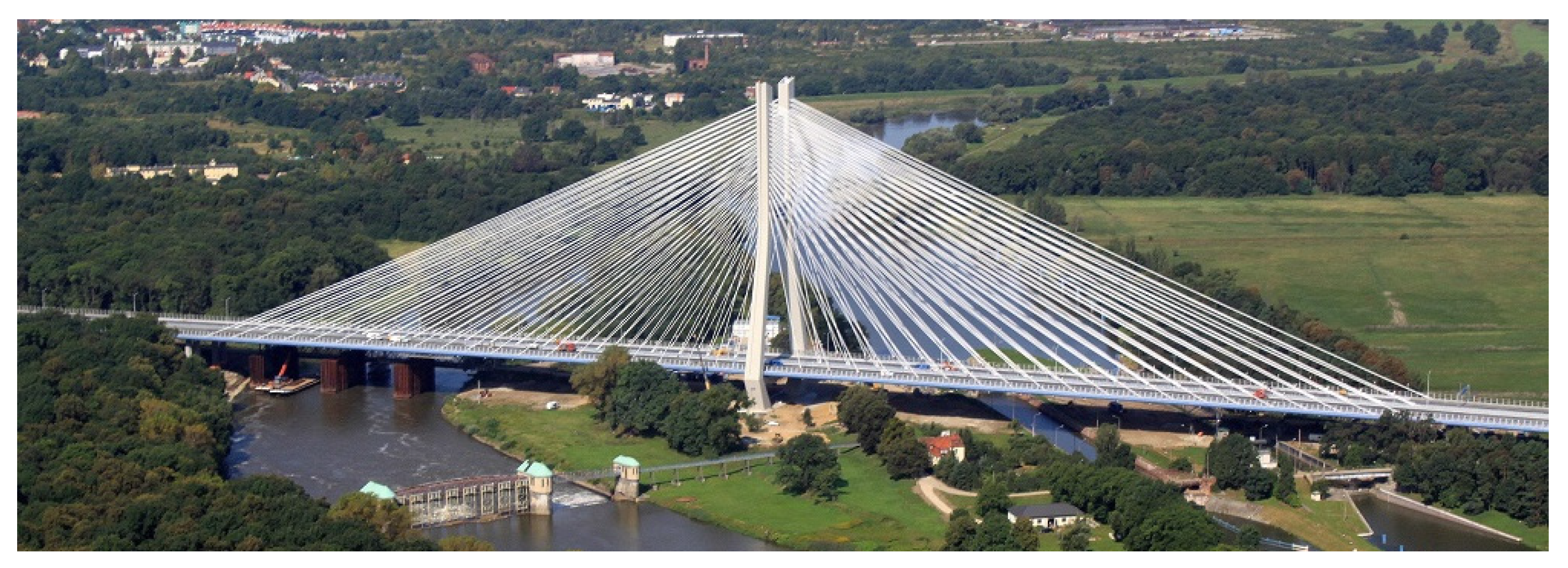
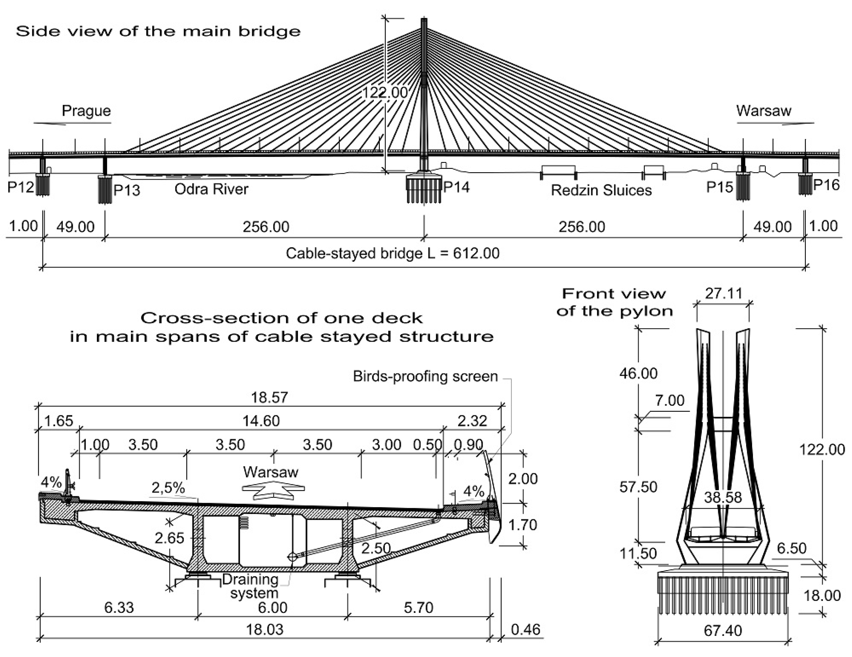
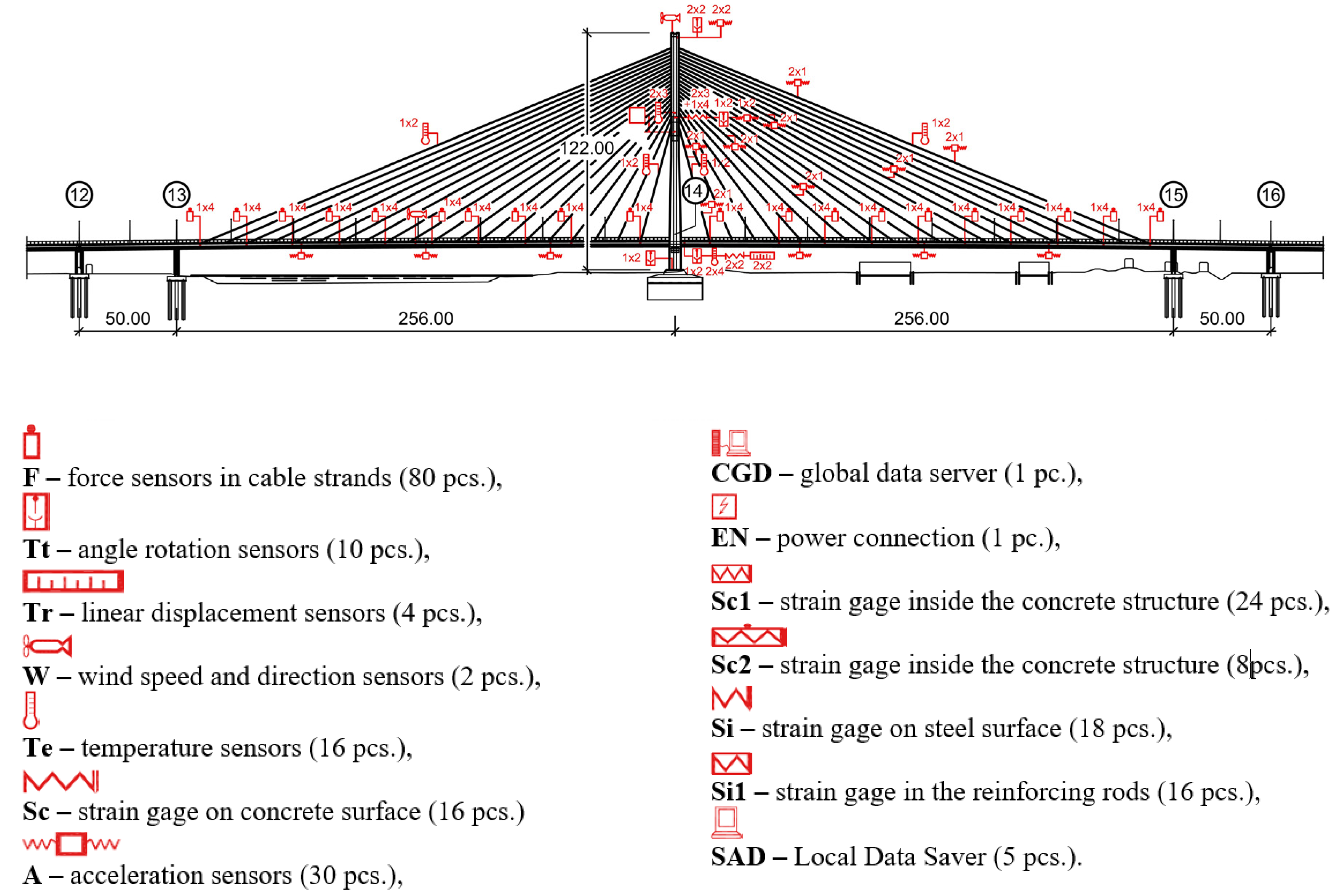
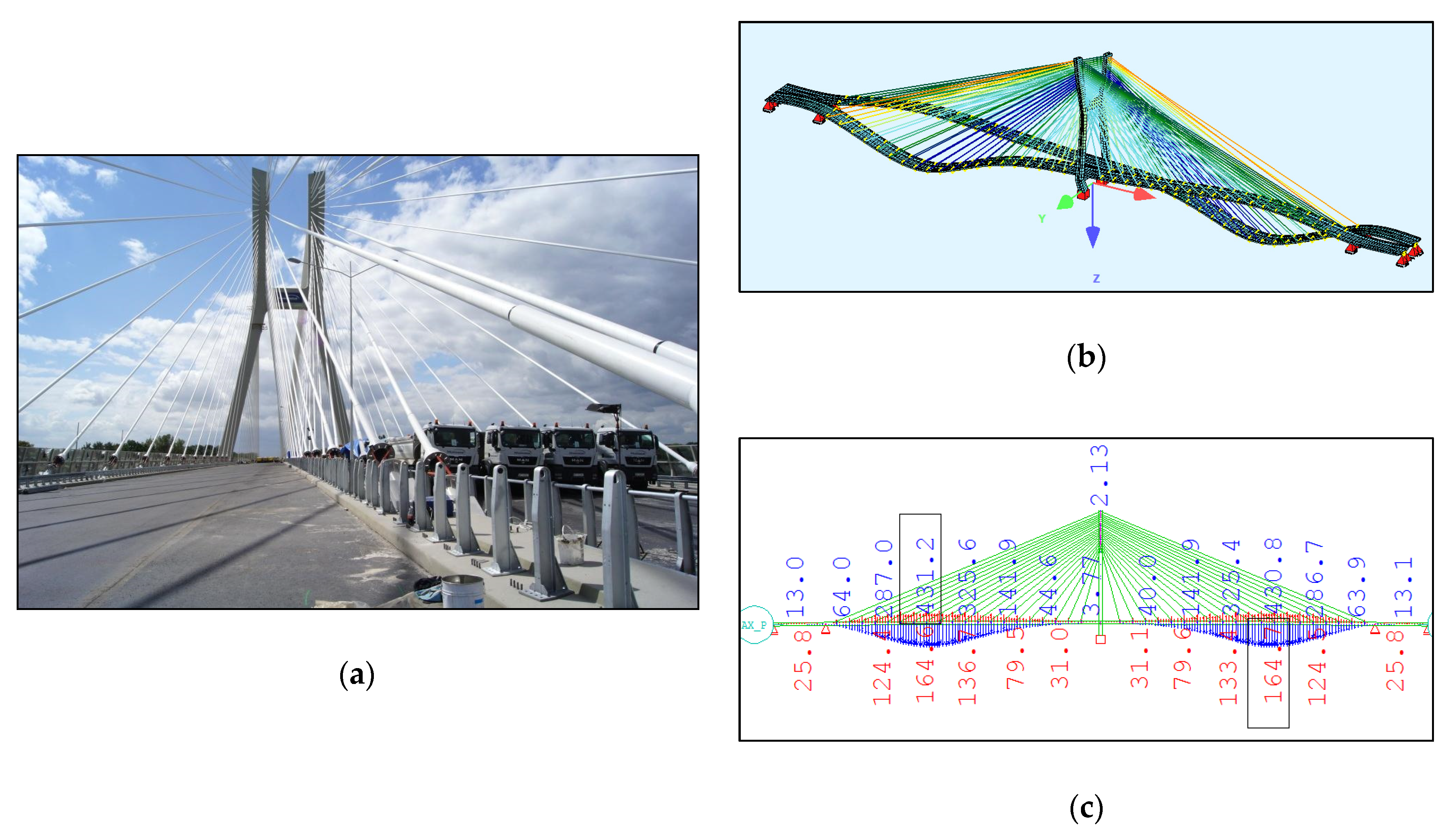
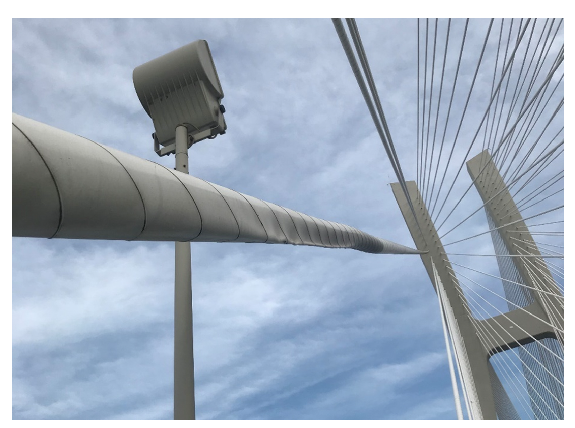
2. The Rędziński Bridge and its SHM System
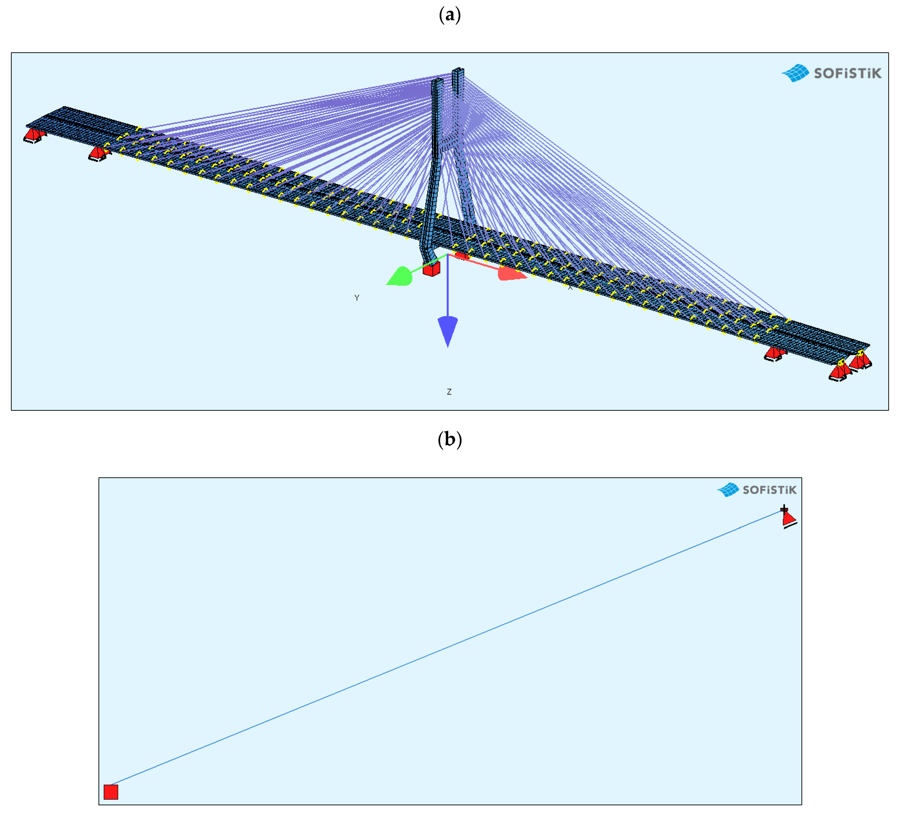
3. The FEM Models
4. Comparison of the Measured Data
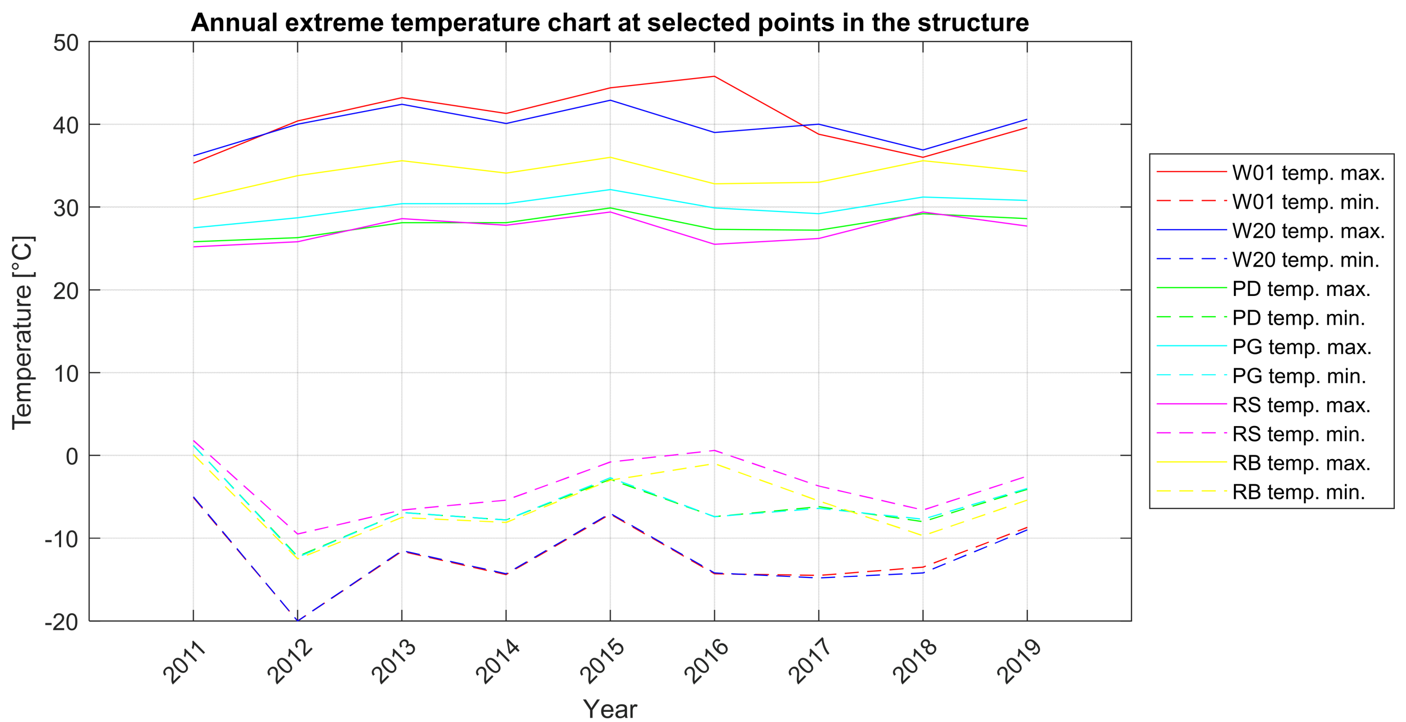
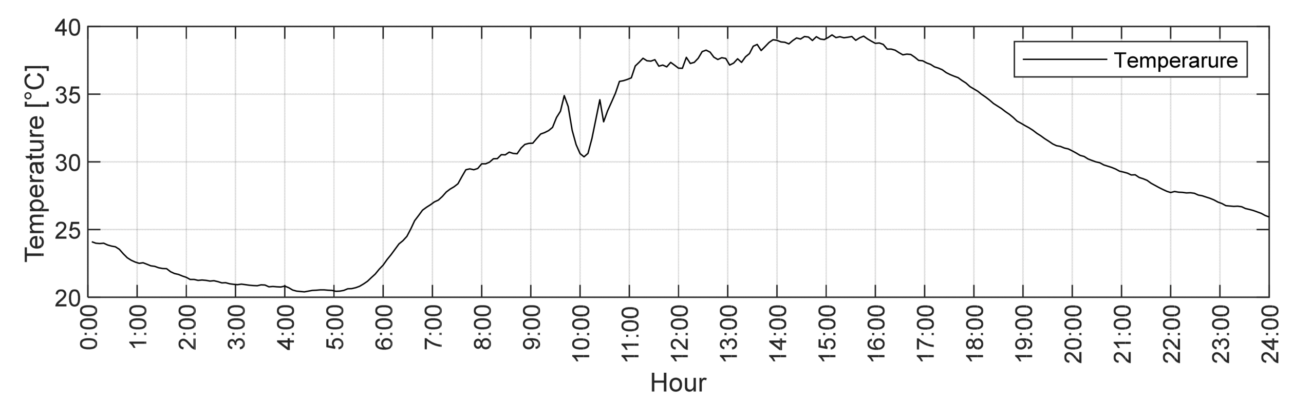
4.1. Temperatures
- the longest stay cable (symbol W-20),
- the shortest stay cable (symbol W-01),
- bottom of the deck section (symbol PD),
- top of the deck section (symbol PG),
- steel in the pylon’s upper cross-beam (RS symbol),
- concrete in the pylon’s upper cross-beam (symbol RB).
4.2. Traffic Loads
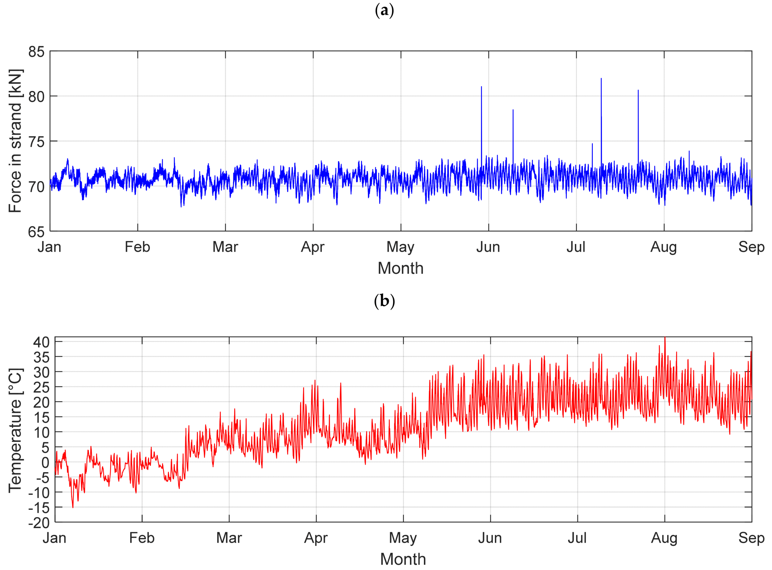
5. Cable Forces Analysis
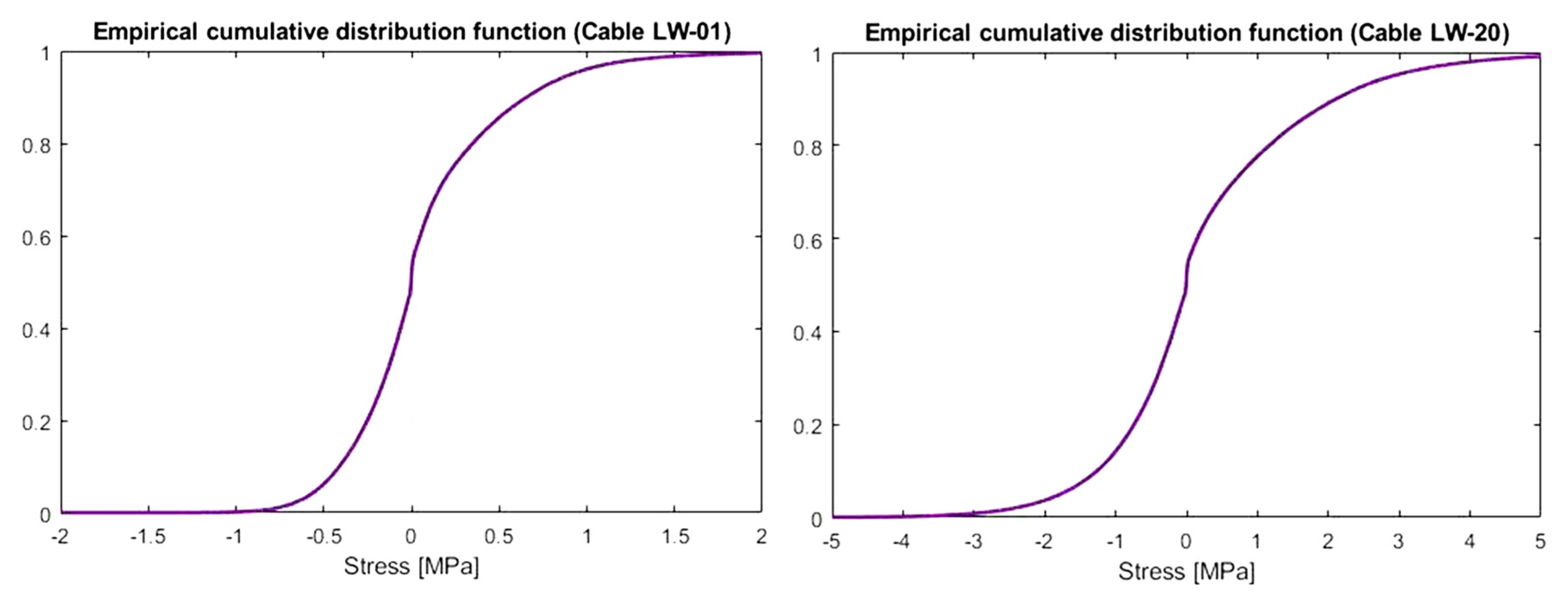
6. Histogram Interpretation
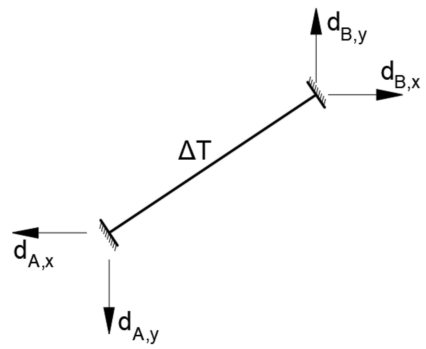
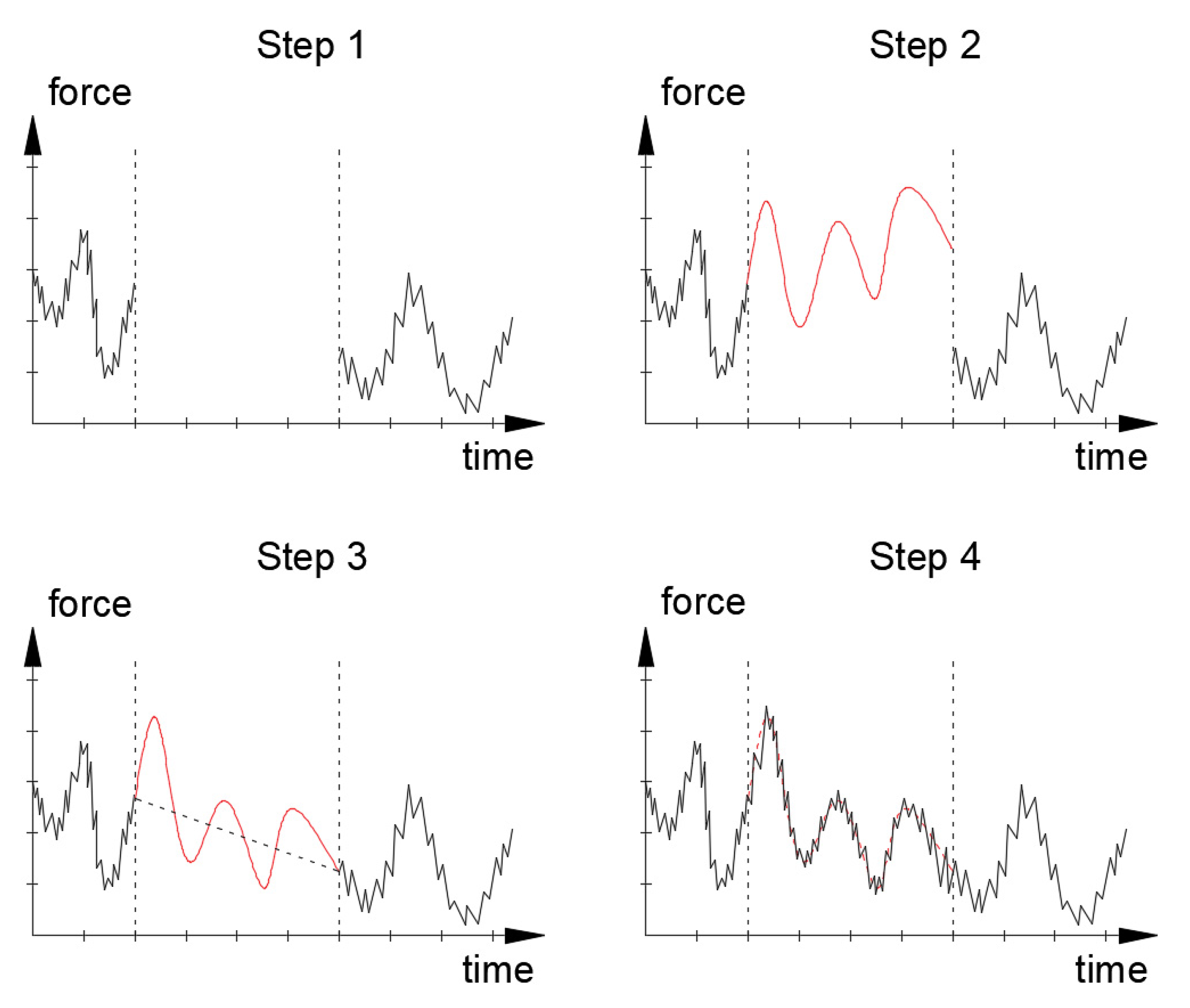
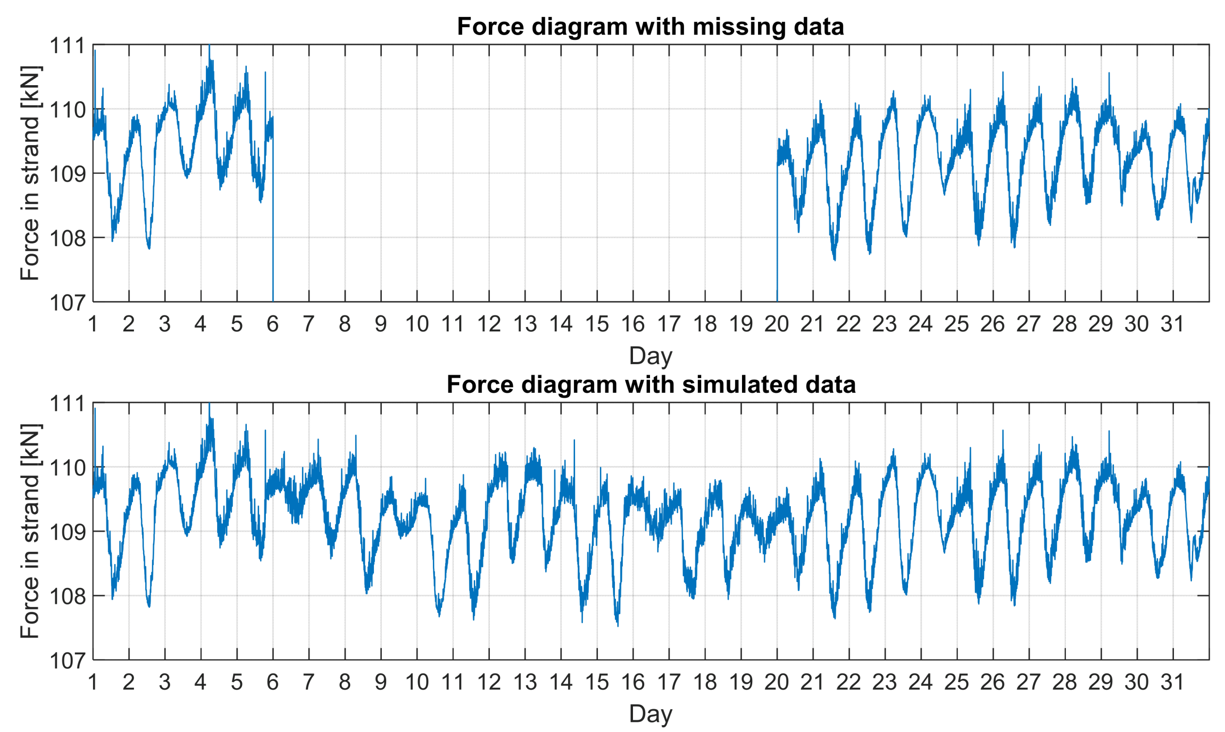
7. Data Simulations
8. Characteristics of the Influence of Individual Loads on the Cable Tension Force
9. Discussion
Author Contributions
Funding
Institutional Review Board Statement
Informed Consent Statement
Data Availability Statement
Acknowledgments
Conflicts of Interest
References
- Wenzel, H. Health Monitoring of Bridges; John Wiley & Sons Ltd.: Chichester, UK, 2009. [Google Scholar]
- Maljaars, J.; Vrouwenvelder, T. Fatigue failure analysis of stay cables with initial defects: Ewijk bridge case study. Struct. Saf. 2014, 51, 47–56. [Google Scholar] [CrossRef]
- Tokujama, S.; Ishihara, S.; Taniyama, S. Full Scale Fatigue Tests for Stay Cable Systems; ETH Zürich: Zürich, Switzerland, 1995. [Google Scholar] [CrossRef]
- Winkler, J.; Georgias, C.; Fischer, G.; Wood, S.; Ghannoum, W. Structural response of a multi-strand stay cable to cyclic bending load. Struct. Eng. Int. 2015, 2, 141–150. [Google Scholar] [CrossRef]
- Winkler, J. Parallel Monostrand Stay Cable Bending Fatigue. Ph.D. Thesis, Technical University of Denmark, Copenhagen, Denmark, 2014. [Google Scholar]
- Biliszczuk, J.; Hawryszków, P.; Teichgraeber, M. Structural health monitoring system of a concrete cable-stayed bridge. Archit. Civ. Eng. Environ. 2018, 11, 69–77. [Google Scholar] [CrossRef]
- Biliszczuk, J.; Barcik, W.; Onysyk, J.; Toczkiewicz, R.; Tukendorf, A.; Tukendorf, K. Rędziński Bridge in Wrocław—The largest concrete cable-stayed bridge in Poland. Struct. Eng. Int. 2014, 24, 285–292. [Google Scholar] [CrossRef]
- Hawryszków, P.; Hildebrand, M. Installation of the largest stay cable system in Poland—the Rędziński bridge in Wrocław. In Proceedings of the 18th IABSE Congress On Innovative Infrastructures—Toward Human Urbanism, Seoul, Korea, 19–21 September 2012. [Google Scholar] [CrossRef]
- Hawryszków, P. Investigation of tension forces in a stay cable systems of a road bridge using vibration methods. In Proceedings of the EVACES’15, 6th International Conference on Experimental Vibration Analysis for Civil Engineering Structures, MATEC Web of Conferences, Zurich, Switzerland, 19–21 October 2015. [Google Scholar] [CrossRef]
- Bień, J.; Kużawa, M.; Kamiński, T. Validation of numerical models of concrete box bridges based on load test results. Arch. Civ. Mech. Eng. 2015, 15, 1046–1060. [Google Scholar] [CrossRef]
- Hildebrand, M.; Nowak, Ł. Measurement of temperature distribution within steel box girder of Vistula River bridge in Central Europe. Balt. J. Road Bridge Eng. 2020, 15, 71–95. [Google Scholar] [CrossRef]
- Kang, F.; Li, J.; Zhao, S.; Wang, Y. Structural health monitoring of concrete dams using long-term air temperature for thermal effect simulation. Eng. Struct. 2019, 180, 642–653. [Google Scholar] [CrossRef]
- Kang, F.; Li, J.; Dai, J. Prediction of long-term temperature effect in structural health monitoring of concrete dams using support vector machines with Jaya optimizer and salp swarm algorithms. Adv. Eng. Softw. 2019, 131, 60–76. [Google Scholar] [CrossRef]
- Caetano, E. Cable Vibrations in Cable-Stayed Bridges, 9th ed.; IABSE International Association for Bridge and Structural Engineering: Switzerland, Zürich, 2007. [Google Scholar]
- Gimsing, N.J.; Georgakis, C.T. Cable Supported Bridges: Concept and Design; John Wiley & Sons, Ltd.: Chichester, UK, 2011. [Google Scholar]
- Greco, F.; Lonetti, P.; Pascuzzo, A. Dynamic Analysis of Cable-Stayed Bridges Affected by Accidental Failure Mechanisms under Moving Loads. Math. Probl. Eng. 2013, 2013, 302706. [Google Scholar] [CrossRef]
- Mankar, A.; Bayane, I.; Sørensen, J.D.; Brühwiler, E. Probabilistic reliability framework for assessment of concrete fatigue of existing RC bridge deck slabs using data from monitoring. Eng. Struct. 2019, 201. [Google Scholar] [CrossRef]
- Szala, G. Application of two-parameter fatigue characteristics in fatigue persistence calculations of structural components under conditions of a broad spectrum of loads. Pol. Marit. Res. 2016, 4, 138–145. [Google Scholar] [CrossRef][Green Version]
- Heywood, R.B. Designing Against Fatigue; Chapman Hall: London, UK, 1962. [Google Scholar]
- Schijve, J. Fatigue of Structures and Materials; Springer: Dordrecht, The Netherlands, 2009. [Google Scholar]
- Panontin, T.; Sheppard, S. (Eds.) Fatigue and Fracture Mechanics; ASTM International: West Conshohocken, PA, USA, 1999; Volume 29. [Google Scholar] [CrossRef]
- Serensen, S.V.; Kogayev, V.P.; Shnejderovich, R.M. Permissible Loading and Strength Calculations of Machine Components; Maschinostroenie: Mosow, Russia, 1975. [Google Scholar]
- Winkelmann, K.; Żyliński, K.; Górski, J. Probabilistic analysis of settlements under a pile foundation of a road bridge pylon. Soils Found. 2020, 61, 80–94. [Google Scholar] [CrossRef]
- Jang, M.; Lee, Y.; Won, D.; Kang, Y.-J.; Kim, S. Static Behaviors of a Long-span Cable-Stayed Bridge with a Floating Tower under Dead Loads. J. Mar. Sci. Eng. 2020, 8, 816. [Google Scholar] [CrossRef]
- Seeram, M.; Manohar, Y. Two-Dimensional Analysis of Cable Stayed Bridge under Wave Loading. J. Inst. Eng. India Ser. A 2018, 99, 351–357. [Google Scholar] [CrossRef]
- Bayane, I.; Brühwiler, E. Structural condition assessment of reinforced-concrete bridges based on acoustic emission and strain measurements. J. Civ. Struct. Health Monit. 2020, 10, 1037–1055. [Google Scholar] [CrossRef]
- Song, G.; Wang, C.; Wang, B. Structural Health Monitoring (SHM) of Civil Structures. Appl. Sci. 2017, 7, 789. [Google Scholar] [CrossRef]
- Svensson, H. Cable-Stayed Bridges, 40 Years of Experience Worldwide; Ernst und Sohn: Berlin, Germany, 2012. [Google Scholar]
- Chakraborty, J.; Katunin, A.; Klikowicz, P.; Salamak, M. Embedded ultrasonic transmission sensors and signal processing techniques for structural change detection in the Gliwice bridge. Procedia Struct. Integr. 2019, 17, 387–394. [Google Scholar] [CrossRef]
- Wang, X.; Chakraborty, J.; Niederleithinger, E. Noise Reduction for Improvement of Ultrasonic Monitoring Using Coda Wave Interferometry on a Real Bridge. J. Nondestruct. Eval. 2021, 40, 14. [Google Scholar] [CrossRef]
- Sheer, J. Failed Bridges: Case Studies, Causes and Consequences; Ernst und Sohn: Berlin, Germany, 2010. [Google Scholar]
- Hui, L.; Shunlong, L.; Jinping, O.; Hongwei, L. Reliability assessment of cable-stayed bridges based on structural health monitoring techniques. Struct. Infrastruct. Eng. 2012, 8, 829–845. [Google Scholar]


 |  | ||||
|---|---|---|---|---|---|
| Stay Cable Number | Number of Strands | Horizontal Length Lh [m] | Vertical Length Lv [m] | Total Length L [m] | |
| 1 | 21 | 24 | 19.06 | 64.64 | 67.39 |
| 2 | 22 | 28 | 30.51 | 67.58 | 74.15 |
| 3 | 23 | 28 | 42.33 | 69.94 | 81.75 |
| 4 | 24 | 30 | 54.29 | 72.03 | 90.20 |
| 5 | 25 | 32 | 66.30 | 74.07 | 99.41 |
| 6 | 26 | 34 | 78.31 | 76.01 | 109.14 |
| 7 | 27 | 38 | 90.37 | 77.95 | 119.35 |
| 8 | 28 | 40 | 102.41 | 79.85 | 129.86 |
| 9 | 29 | 46 | 114.45 | 81.75 | 140.65 |
| 10 | 30 | 48 | 126.51 | 83.62 | 151.64 |
| 11 | 31 | 48 | 138.54 | 85.52 | 162.81 |
| 12 | 32 | 48 | 150.57 | 87.41 | 174.10 |
| 13 | 33 | 48 | 162.61 | 89.29 | 185.51 |
| 14 | 34 | 48 | 174.59 | 91.16 | 196.96 |
| 15 | 35 | 48 | 186.63 | 93.06 | 208.55 |
| 16 | 36 | 48 | 198.66 | 94.97 | 220.20 |
| 17 | 37 | 48 | 210.70 | 96.90 | 231.91 |
| 18 | 38 | 48 | 222.75 | 98.84 | 243.70 |
| 19 | 39 | 48 | 234.79 | 100.77 | 255.50 |
| 20 | 40 | 40 | 246.82 | 102.71 | 267.34 |
| Measured Quantity | Sample Mark | Description |
|---|---|---|
| Force in the stay cable | W16-LW/F | The sensor located in the stay cable No. 16 (W16), which supports the left deck (L) from the inside (W), measuring the tension force of the stay cable (F). |
| Temperature | W21-LZ/Te | The sensor located on the stay cable No. 21 (W21), on the left deck (L) from the outside (Z), measuring the temperature (Te). |
| No. | Description | Function | Photo * |
|---|---|---|---|
| 1. | Vibrating wire strain gages integrated with temperature sensors: Geokon model 4000 | Strain and temperature measurements in the pylon and decks |  |
| 2. | Vibrating wire strain gages integrated with temperature sensors: Geokon model 4100/4150 | Strain and temperature measurements in the pylon and decks |  |
| 3. | Vibrating wire strain gages integrated with temperature sensors: Geokon model 4420 | Measurement of linear displacements |  |
| 4. | Accelerometers: Haneywell model MA321 | Measurement of structure accelerations |  |
| 5. | Temperature sensors: Geokon model 3800 | Temperature measurement of individual elements of the structure |  |
| 6. | Vibrating wire tiltmeters: Geokon model 6350 | Measurement of angular displacements |  |
| 7. | Force sensor: Advitam Permanent Monostrand Load Cell Model MLC C P | Measurement of forces in stay cables |  |
| Form Number | Frequency Number and Form | FEM [Hz] | Tests [Hz] |
|---|---|---|---|
| 1. |  | 0.25 | 0.25 |
| 2. |  | 0.32 | 0.31 |
| 3. |  | 0.50 | 0.48 |
| 4. |  | 0.51 | 0.48 |
| 5. |  | 0.61 | 0.62 |
| Element | Lowest Daily Average Temperature in January 2017 (°C) | Highest Daily Average Temperature in August 2017 (°C) | ΔT (°C) |
|---|---|---|---|
| decks | −2.40 | 22.90 | +25.30 |
| pylon | −2.40 | 22.80 | +25.20 |
| cables | −8.35 | 26.00 | +34.35 |
| Position | The Shortest Cable (LZ-W21) (kN) | The Shortest Cable (LW-W1) (kN) | The Longest Cable (LZ-W20) (kN) | The Longest Cable (LW-W20) (kN) |
|---|---|---|---|---|
| Highest daily average force in January 2017 (06/01/17) | 63.14 | 51.82 | 73.17 | 68.31 |
| Lowest daily average force in August 2017 (18/08/17) | 62.80 | 51.04 | 73.04 | 67.91 |
| ΔF (SHM) | −0.34 | −0.78 | −0.13 | −0.40 |
| ΔF (FEM) | −2.60 | −2.63 | −4.25 | −4.21 |
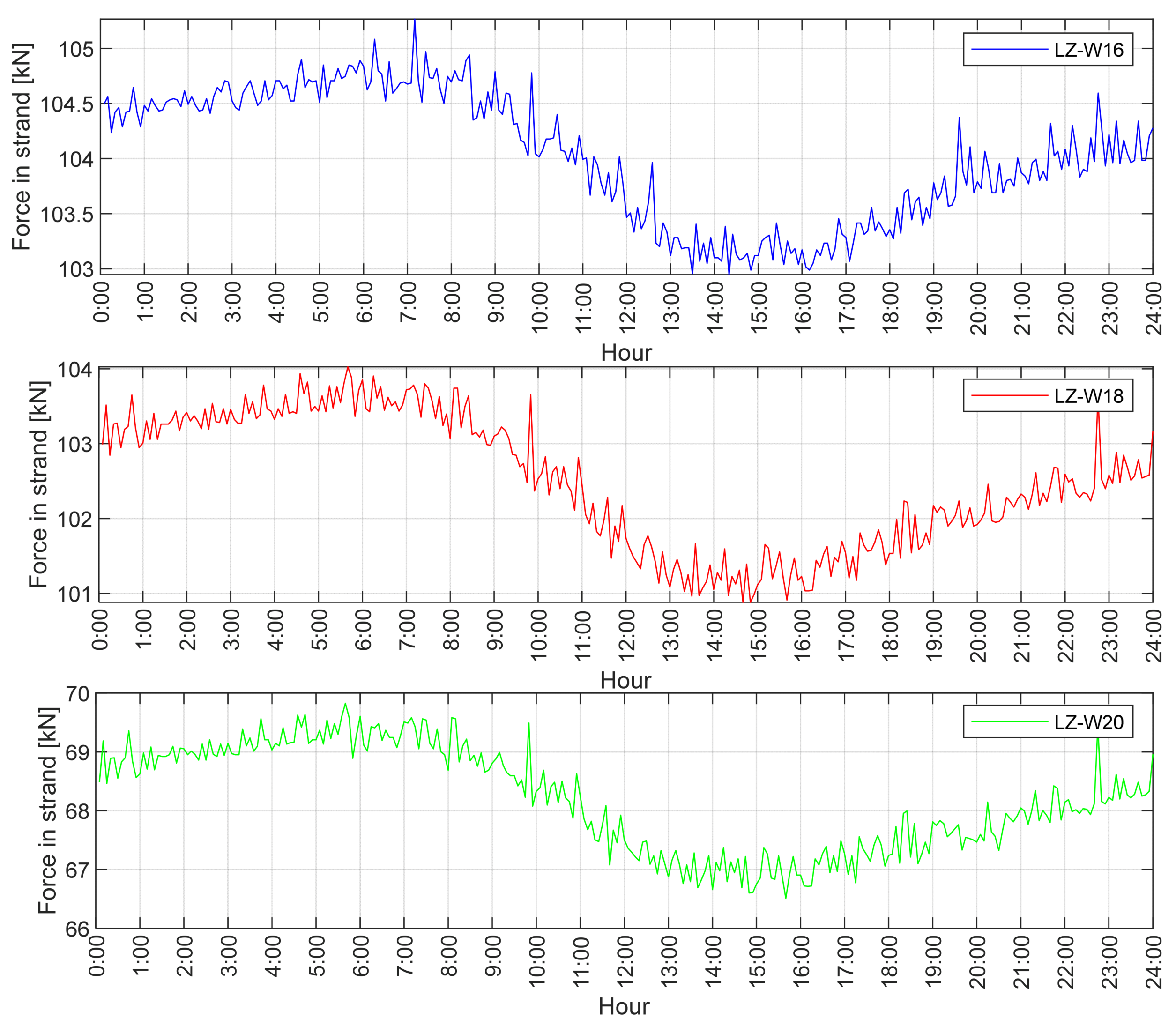
| Cable Number | Initial Force (kN) | Maximum Force Range (kN) | Minimum Force Range (kN) | −ΔT (°C) | +ΔT (°C) | Calculated Maximum Force (kN) | Calculated Minimum Force (kN) |
|---|---|---|---|---|---|---|---|
| LZ-W16 | 104.5 | 104.7–105.3 | 102.9–103.4 | −3.7 | +15.3 | 104.91 | 102.78 |
| LZ-W18 | 103.5 | 103.4–104.4 | 100.9–101.3 | −3.7 | +15.3 | 103.41 | 101.28 |
| LZ-W20 | 68.5 | 69.3–69.9 | 66.5–67.2 | −3.7 | +15.3 | 69.31 | 67.18 |
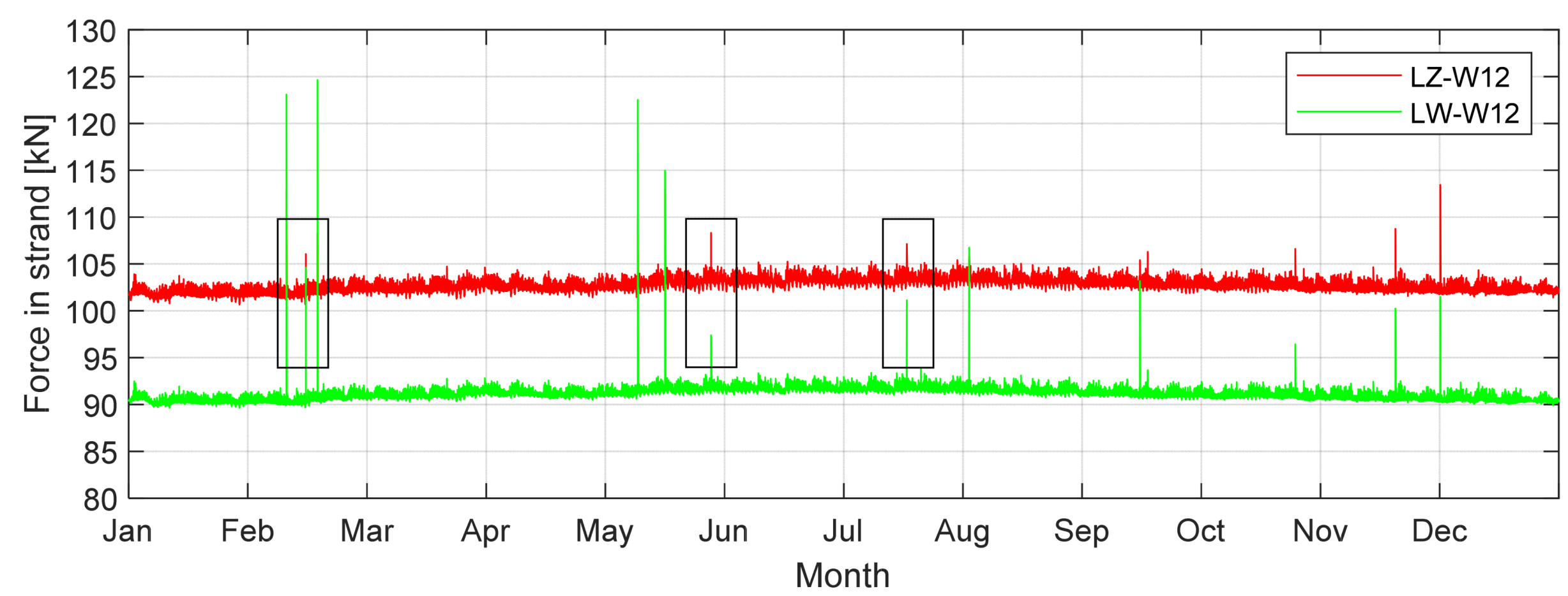
| Peak Number (Month) | Peak Value | Monthly Average Strand Force | Force Difference in Strand | Force Difference in Cable (48 Strands) | Estimated Loading on Whole Deck | Example Vehicles |
|---|---|---|---|---|---|---|
| 1 (February) | 101.8 kN | 97.3 kN | 4.5 kN | 216.0 kN | 360 t | 3 loaded concrete mixers (3 × 40 t) + 10 lorries (10 × 15 t) and cars |
| 2 (May) | 103.6 kN | 97.9 kN | 5.7 kN | 273.6 kN | 460 t | Military transport (e.g., Stanag MLC 150) + lorries (15 t) and cars |
| 3 (July) | 105.0 kN | 98.0 kN | 7.0 kN | 336.0 kN | 570 t | Military transport (e.g., Stanag MLC 150) + lorries (15 t) and cars |
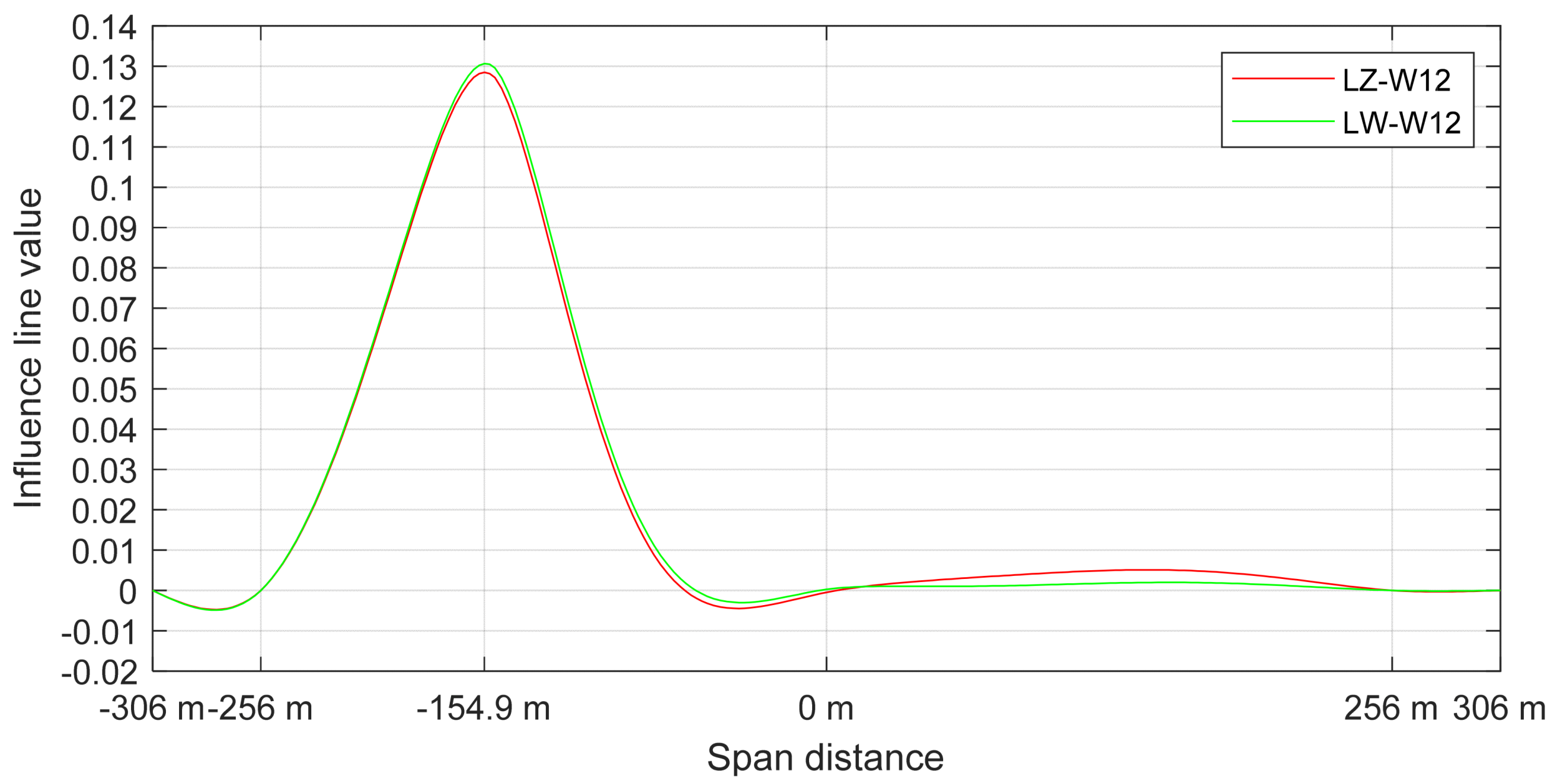
| Stay Cable Number | Force Change Calculated from Influence Lines | Force Change Read from the FEM Model during the Dynamic Crossing |
|---|---|---|
| LZ-W12 | 1.07 kN | 1.20 kN |
| LW-W12 | 1.05 kN | 0.94 kN |
| Cable | SSE | R-Sqr | RMSE |
|---|---|---|---|
| LZ-W20 | 1.2 | 0.984 | 0.067 |
| LZ-W16 | 2.1 | 0.981 | 0.089 |
| LZ-W01 | 5.4 | 0.976 | 0.141 |
| Stay Cable | Ds | Da | Ds/Da |
|---|---|---|---|
| LZ-W01 | 16,705.2 | 13,983.9 | 1.19 |
| LZ-W16 | 34,320.3 | 28,593.4 | 1.20 |
| LZ-W20 | 52,831.9 | 44,848.1 | 1.18 |
| Probability Distribution Function (PDF) | Distribution Parameters | |
|---|---|---|
| Average stress | Normal | σ—average value µ—standard deviation |
| Stress amplitudes | Weibull | λ—scale parameter k—shape parameter |
| Year | Cable LW-20 | Cable LW-16 | Cable LW-01 |
|---|---|---|---|
| 2011 | 0.00 | 0.00 | 0.00 |
| 2012 | 0.00 | 0.00 | 0.00 |
| 2013 | 1.71 × 10⁻⁶ | 7.57 × 10⁻⁷ | 1.74 × 10⁻⁹ |
| 2014 | 3.48 × 10⁻⁶ | 1.46 × 10⁻⁶ | 3.67 × 10⁻⁹ |
| 2015 | 5.62 × 10⁻⁶ | 1.97 × 10⁻⁶ | 4.73 × 10⁻⁹ |
| 2016 | 8.04 × 10⁻⁶ | 2.58 × 10⁻⁶ | 5.88 × 10⁻⁹ |
| 2017 | 1.08 × 10⁻⁵ | 3.33 × 10⁻⁶ | 7.32 × 10⁻⁹ |
| 2018 | 1.43 × 10⁻⁵ | 4.15 × 10⁻⁶ | 8.85 × 10⁻⁹ |
| 2025 * | 8.75 × 10⁻⁵ | 2.15 × 10⁻⁵ | 4.24 × 10⁻⁸ |
| 2050 * | 5.02 × 10⁻³ | 5.80 × 10⁻⁴ | 1.26 × 10⁻⁶ |
| 2075 * | 3.89 × 10⁻² | 2.83 × 10⁻³ | 6.30 × 10⁻⁶ |
Publisher’s Note: MDPI stays neutral with regard to jurisdictional claims in published maps and institutional affiliations. |
© 2021 by the authors. Licensee MDPI, Basel, Switzerland. This article is an open access article distributed under the terms and conditions of the Creative Commons Attribution (CC BY) license (http://creativecommons.org/licenses/by/4.0/).
Share and Cite
Biliszczuk, J.; Hawryszków, P.; Teichgraeber, M. SHM System and a FEM Model-Based Force Analysis Assessment in Stay Cables. Sensors 2021, 21, 1927. https://doi.org/10.3390/s21061927
Biliszczuk J, Hawryszków P, Teichgraeber M. SHM System and a FEM Model-Based Force Analysis Assessment in Stay Cables. Sensors. 2021; 21(6):1927. https://doi.org/10.3390/s21061927
Chicago/Turabian StyleBiliszczuk, Jan, Paweł Hawryszków, and Marco Teichgraeber. 2021. "SHM System and a FEM Model-Based Force Analysis Assessment in Stay Cables" Sensors 21, no. 6: 1927. https://doi.org/10.3390/s21061927
APA StyleBiliszczuk, J., Hawryszków, P., & Teichgraeber, M. (2021). SHM System and a FEM Model-Based Force Analysis Assessment in Stay Cables. Sensors, 21(6), 1927. https://doi.org/10.3390/s21061927