2.1. Experimental Setup and Wear-Noise Generation Scheme
Authors have used the experimental rig as described in their recent work on noise and wear correlation [
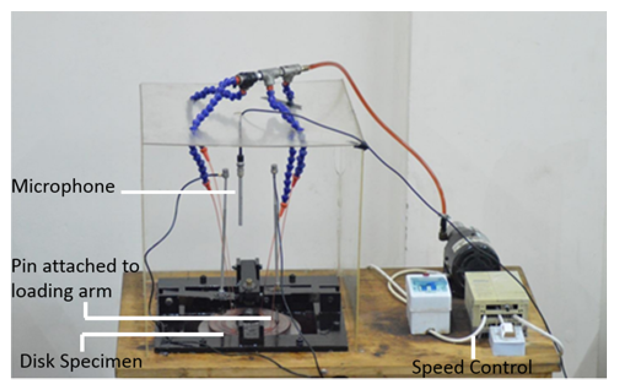
1]. In total, 37 experiments were performed on a pin on disc tribometer as shown in
Figure 1 and considered for the statistical model development and validation.
The tribometer was composed of metallic arms to act as pin holders. A circular mild steel disc was mounted on a shaft and motor assembly that allowed the disc to rotate at a constant speed of 250 rpm. A high speed steel material pin was used and assembled with the help of the pin holder in a way so that it made a prefect mechanical contact with the circular disc as shown in
Figure 1. The pin had a diameter of 5
and a contact diameter of
mm. Additional details about the pin’s material are listed in
Table 1.
The pin tip at contact was made semi-circular in shape. It was assumed that the pin would not be worn out under sliding conditions at any time of experiments and hence the change in airborne noise would only be caused due the surface wear of the disc as it was made of a softer material. Threads of up to 10 in length were present on the other end of the pin, which were used to mount metallic weights and allowed to provide a tangential loading condition on the pin and disc contact during experiments. An oil pump was also used to provide lubrication at the contact and at a rate of 5 mL/s. The selected grade of lubricant was 10W-30 with a density of 877 kg/m.
The noise was recorded by a GRAS 40PP free-field microphone (GRAS Sound & Vibration, Holte, Denmark). The frequency range of the selected microphone was 20 kHz, and it was able to record noises with an upper limit of 128 db. It was vertically placed at the center of the disc as shown in
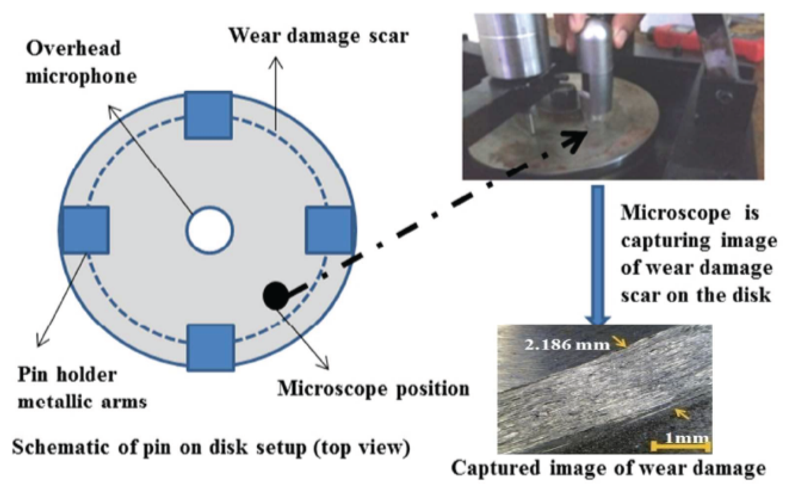
Figure 1. The raw noise signals were acquired by an NI 9234 data acquisition module (National Instruments, Austin, TX, USA) in terms of sound pressure (units pascal) and sampling rate of 25.6 kHz. Images of the wear scars on the disc were taken from six different positions, the same as it was performed in the previous work, with a portable microscope (Dino-Lite AM413T, AnMo Electronics Corporation, Hsinchu, Taiwan) at a magnification of 200× as shown in
Figure 2 [
1].
Using ASTM standard G99 (Standard Test Method for Wear Testing with a Pin-on-Disc Apparatus), disk volume loss
V due to wear scar was calculated [
17]. The wear scar sliding length measurements were measured from the captured images and used in ASTM standard formulation as provided in Equation (
1):
where
R = wear track radius,
d = wear track width,
r = pin end radius, and
V is the volumetric wear, assuming no significant pin wear.
The load and lubrication specification breakdown for the 37 experiments is given in
Table 2. The duration of each experiment was 6 min, with the wear on a disc measured after 30 s intervals, thus resulting in a total of 444 measurements.
2.2. Signal Analysis and Feature Extraction
Cutting processes tend to be stochastic [
30] with generated noise consequently dependent upon the progression of the tool wear [
31]. Hence, the stationarity of the collected data needs to be determined in order to decide the features extraction methodology. If the acquired signals turn out to be non-stationary, then Time-Frequency features would need to be computed; otherwise, frequency domain features would suffice [
32]. To help with the analysis for stationarity, the mean and Autocorrelation Sequence (ACS) of one of the 30 s measurements was computed. The ACS of a process
X can be defined as:
where
n is the time index,
k the lag index, and
E the expectation operator. Hence, the ACS is a measure of the correlation between two samples of the same stochastic process separated by a lag
k.
The evolution of the mean of a 30 s long measurement, computed using a moving average, is plotted against time in
Figure 3.
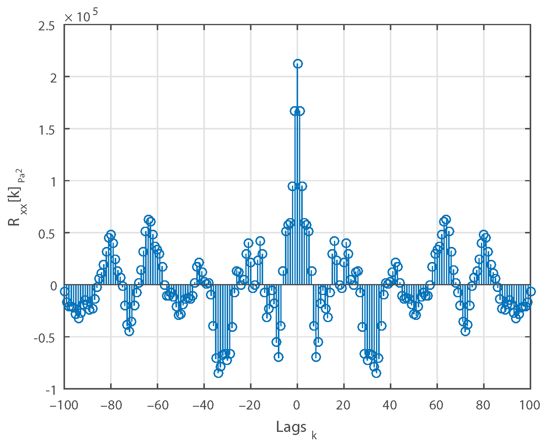
Figure 4 shows the computed ACS against the lag indexes for the same measurement.
Figure 5 displays the same ACS with the lag index limited to
. Observing the three figures, we can conclude that:
The mean is relatively constant.
For , is positive.
is an even function.
is .
approaches as k increases.
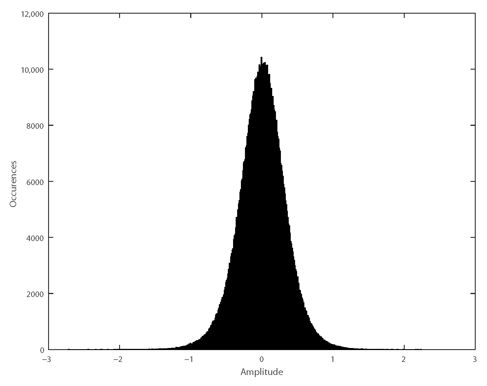
Hence, the measurement can be classified as a wide-sense stationary (WSS) process [
33]. Moreover, since the measured signal resembles a Gaussian distribution, as seen in
Figure 6, this WSS process can be considered strict stationary (SS) as well [
34].
Given the result of the stationarity analysis, the power spectral density (PSD) can be estimated. According to the Wiener–Khinchin theorem, the PSD is the squared discrete Fourier transform (DFT) of the ACS of each measurement signal [
35]. The conventional periodogram estimator is considered analogous to this definition [
36].
Since using the periodogram would have resulted in large fluctuations around the actual PSD due to the method’s inherent asymptotic noise [
37], it is imperative to revert to techniques that reduce spectral variance.
Hence, the Welch method [
38], which involves the segmentation of the signal being analyzed, and averaging of periodograms can be used. While segmentation reduces spectral resolution, the use of segment overlap mitigates this reduction when compared to the Bartlett method for the same number of segments [
39]. The subsequent generation of redundant spectral information due to the use of overlapping is attenuated through the application of a windowing function, such as the Hamming window [
40], over each segment. The Welch method for PSD estimation can be summarized in the following steps:
For periodograms
, a segment
k is defined as:
with
M being the length of each segment and
D controlling the degree of overlap. The number of periodograms involved,
K, is dependent upon the previous two parameters and,
N, the total length of the signal.
Each periodogram can be defined as:
where
Z is the normalization factor considered due to the introduction of the Hamming window function
. By averaging this ensemble of periodograms, the Welch estimator is defined as:
For each measurement of duration 30 s, a Welch estimator with was used along with an overlap of . Since sampling frequency used was , . Consequently, the PSD estimates have a spectral resolution of 20 Hz. A lower window length wasn’t set in order to prevent spectral smearing and higher bias.
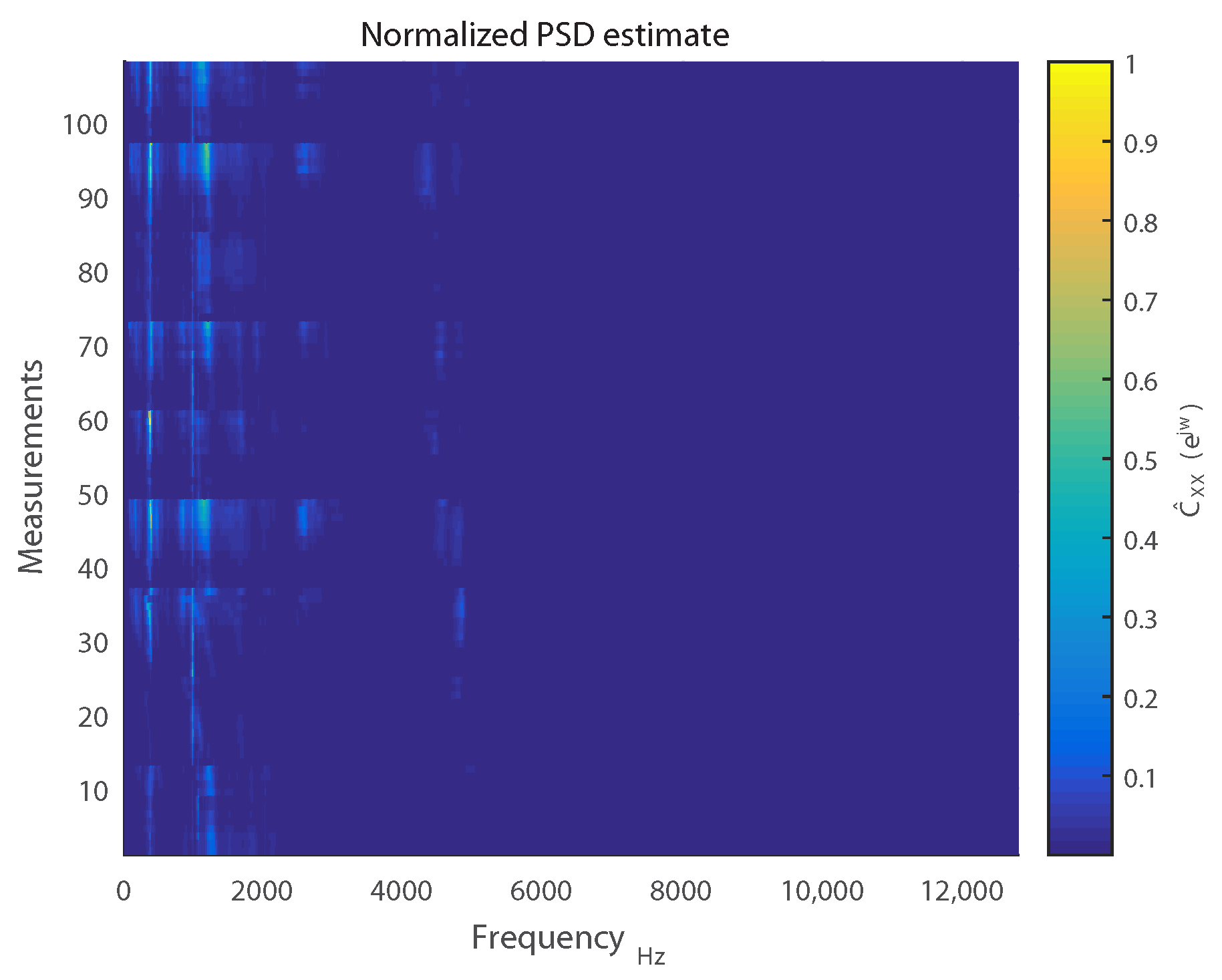
For the measurements we recorded, it was observed that the frequency ranges of interest were
3
and
5
. This can be visualized in
Figure 7, which displays
for 108 measurements of 30 s each. For the sake of visual brevity, only measurements corresponding to absence of load and lubrication have been included.
The identification of these spectral regions of interest led to selection of the PSD estimates of 200 discrete frequency bins as features for our eventual surface wear prediction model.
2.3. Prediction Model Formulation
Since volumetric loss of one disc was measured over a span of 6 min in intervals of 30 s, they are cyclically cumulative, and the task of surface wear prediction can be modeled as a time series forecasting problem with a time horizon [
41] of depth 12.
For subsequent discussion, let
h denote the time horizon, with
and
corresponding to the surface wear and spectral features of the measurement at horizon
h. The model for predicting surface wear estimates
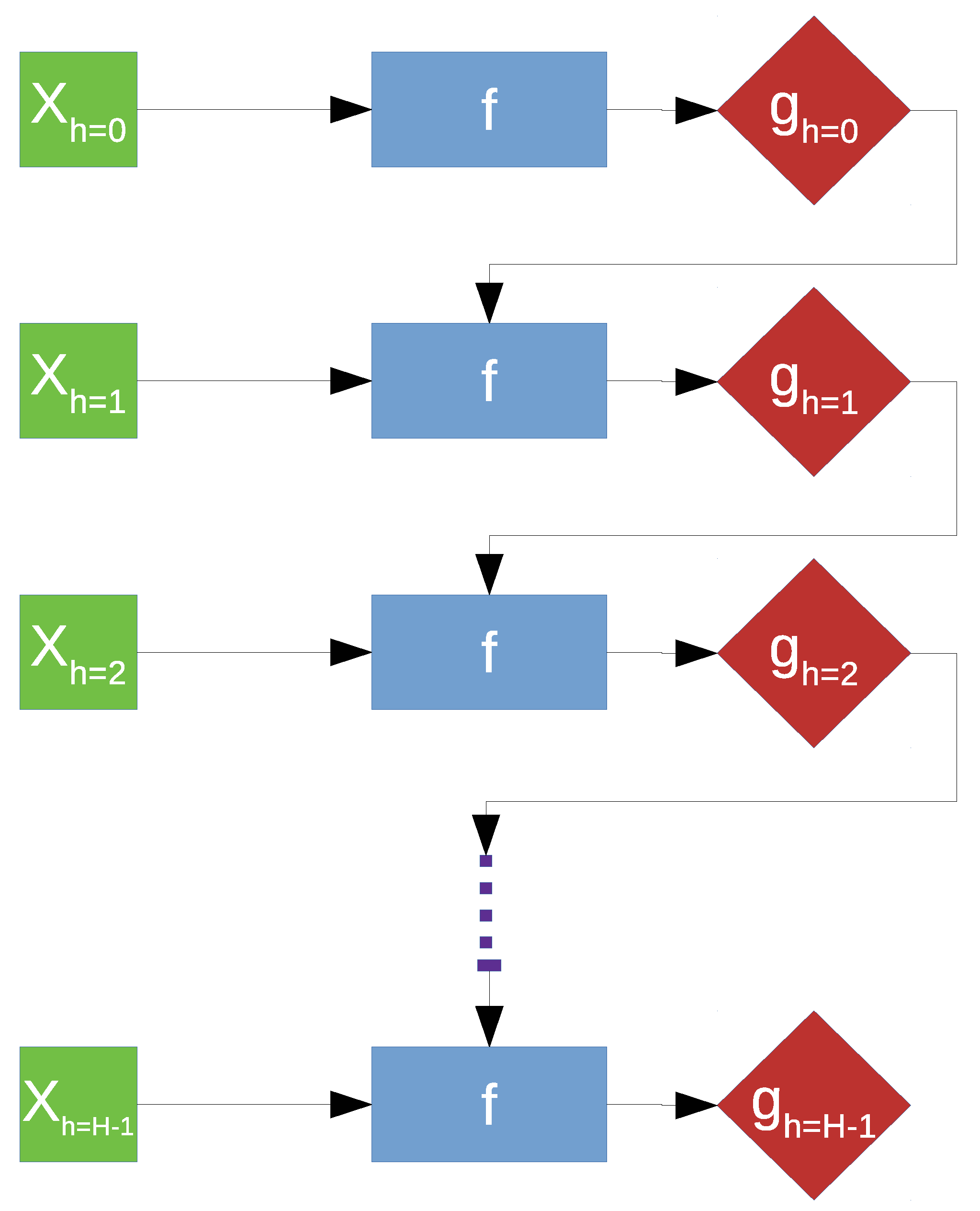
can be expressed as
f. A common solution for a forecasting problem is the recursive approach, which involves the prediction being fed back to the model, hence the name, as part of the input for prediction of the target belonging to the next time horizon [
42]. However, this approach, illustrated in
Figure 8, is extremely sensitive to prediction error due to error propagation [
43].
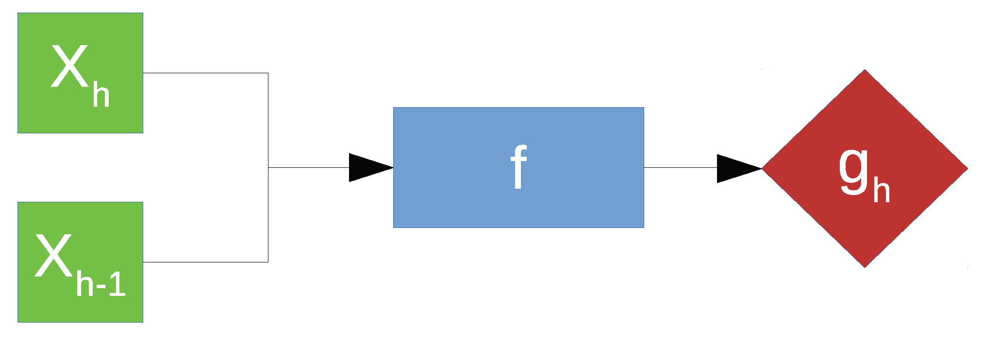
However, the time series aspect of the problem could not be ignored since the quantity to be predicted is the cumulative surface wear, with each 30 s wear process dependent on the previous one. Hence, we implemented time-embeddings using a sliding window approach for our spectral feature s [
44]. Consequently, we arrive at a regression problem defined in
Figure 9.
A sliding window, consisting of inputs belonging to the current time horizon h and the previous one , is used as the new inputs which will be used to predict the cumulative surface wear at horizon h. In other words, we have set up a high dimensional regression problem with 400 spectral features as input for every cumulative surface wear output.
2.4. Choice of Regression Models
As can be discerned in
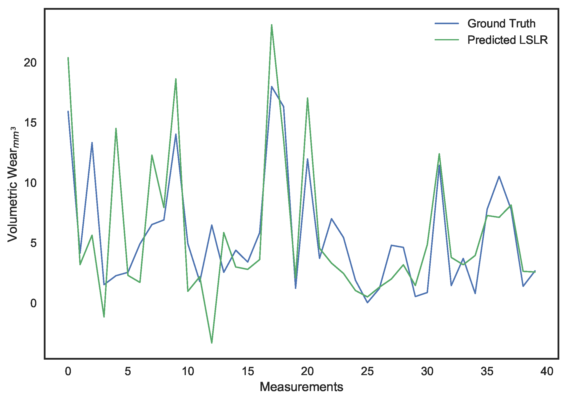
Figure 7, the spectral features exhibit collinearity due to similar PSD estimates between some neighboring discrete frequency bins. Accordingly, a least-squares (LS) linear regression based model will not be optimal for prediction [
45]. An optimal solution will seek to constrict the effects of collinearity between these features by attenuating the weights assigned to them during regression [
46]. One method would be to implement a subset selection of features. However, this approach exhibits high variance due to the binary process of picking or dropping a feature entirely. Consequently, this would result in negligible improvement in prediction performance [
46].
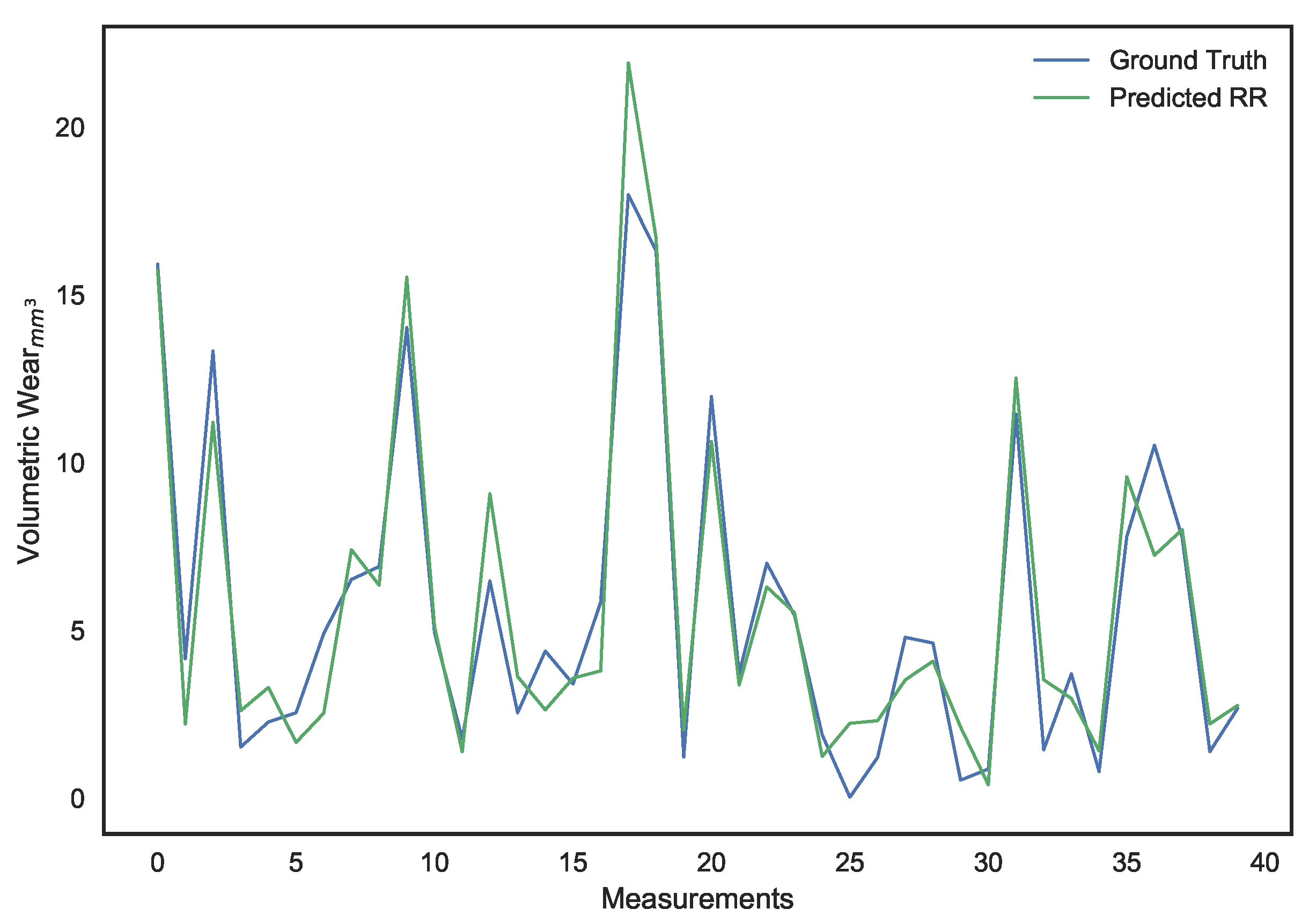
Ridge regression [
47] is the alternate approach that can be adopted. It is a technique involving the shrinking of feature weights by imposing a penalty on their sizes. For a regression model defined by Equation (
7), where
is an input matrix of features,
is the vector of output targets, and
the vector of weights assigned to features:
The LS linear regression solution would be the set of weights that minimize the sum of squared errors between the targets and predictions, as defined in Equation (
8):
Comparatively, the optimization function for ridge regression includes the additional
parameter in order to penalize the size of weights as discussed previously. Hence, converging to the solution for Equation (
9), requires reduction in the magnitudes of feature weights.
While this causes an estimation bias, it decreases prediction error due to a reduction in variance [
48]. The superiority of this method over feature subset selection has been proven in the work of Frank and Friedman (1993) [
49].
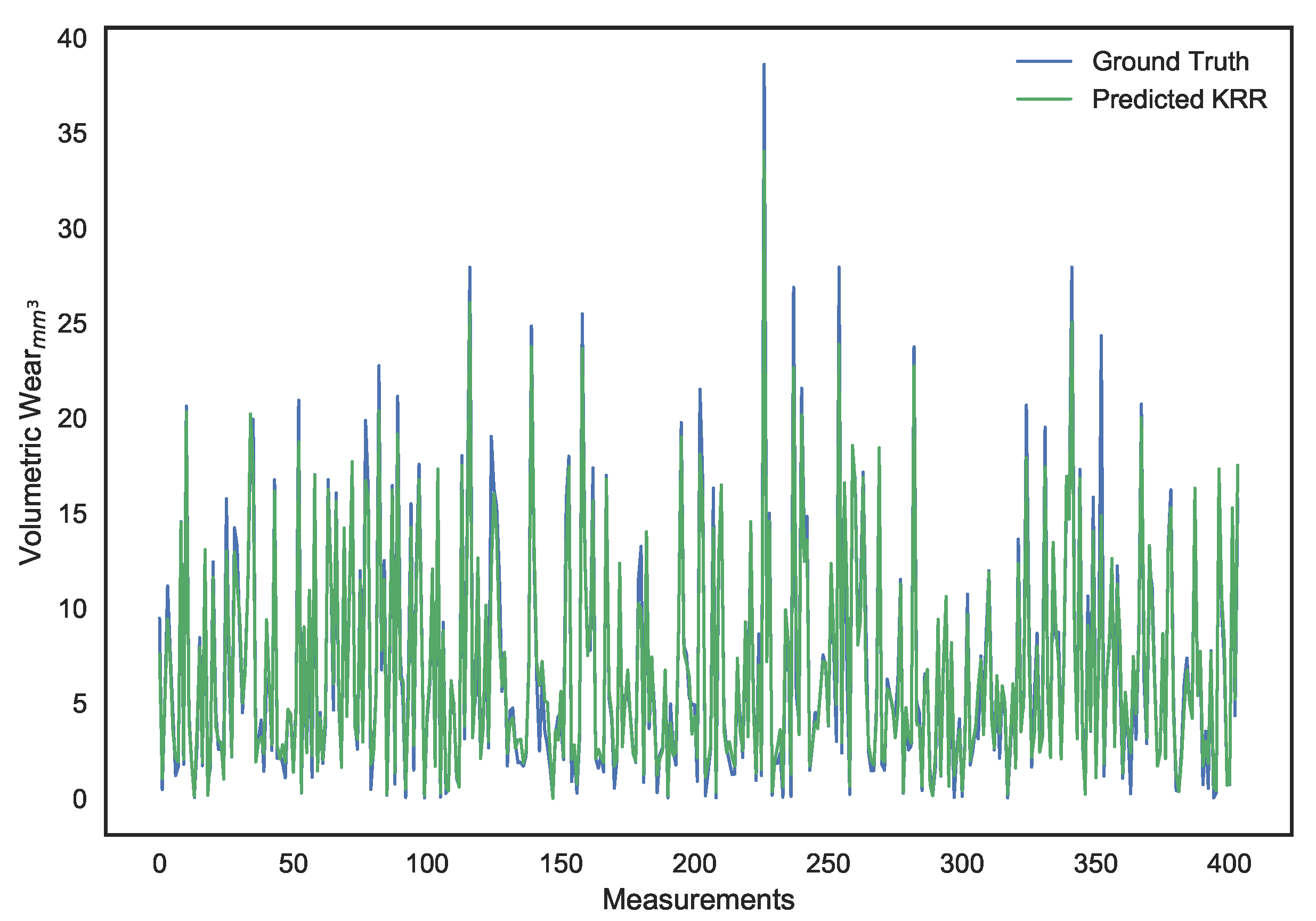
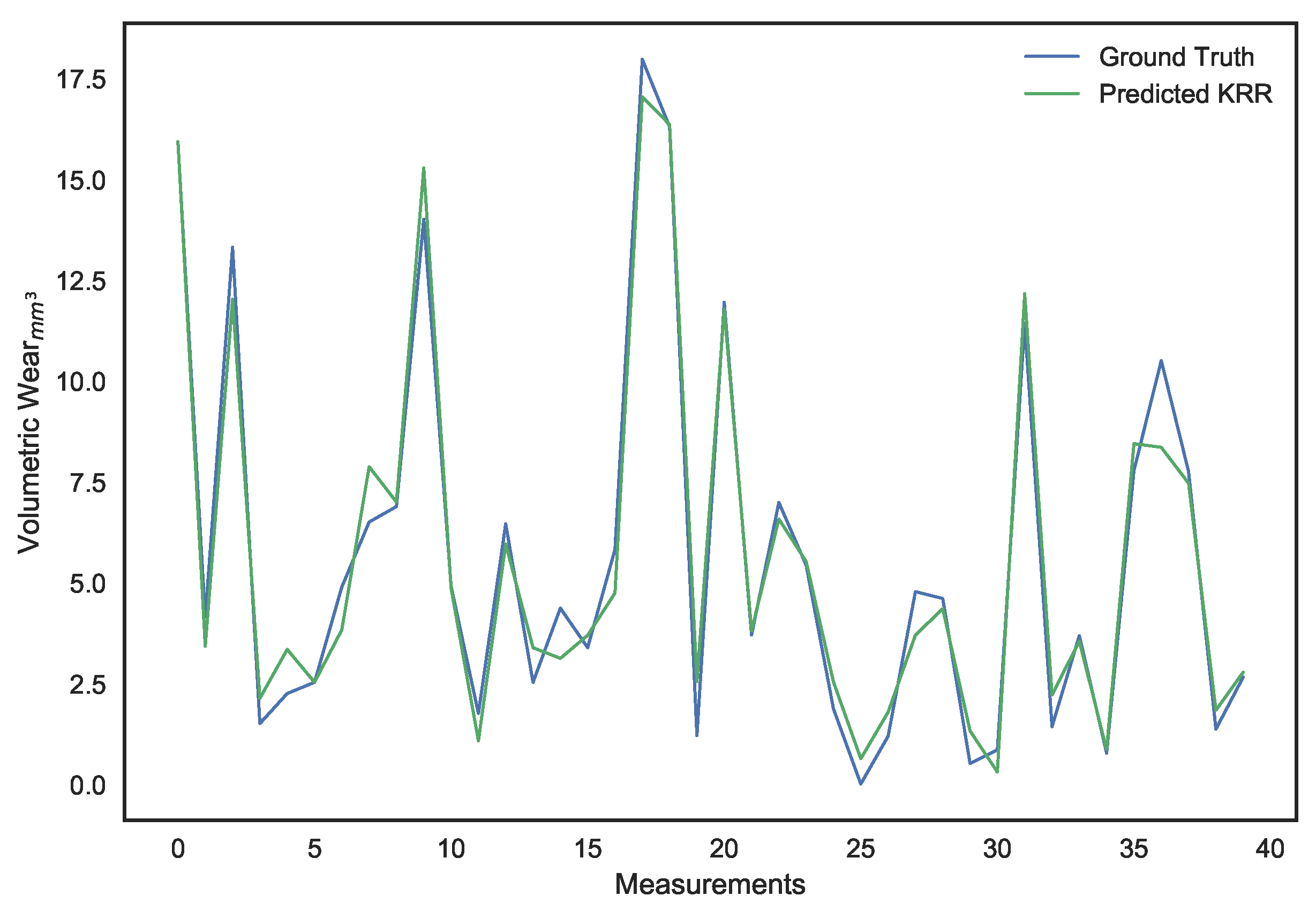
Both LS linear regression and ridge regression suffer from a common drawback, the underlying linearity assumption. Accordingly, they offer poor and highly biased predictions when the relationship between features and the target is more complex. To overcome this issue, we will be moving on from the ridge regression method to Kernel Ridge Regression (KRR) [
50], through which our spectral features will be mapped into a different dimensional space using a nonlinear kernel.
The Chi-Squared (
) kernel [
51], defined in Equation (
10), is used. The kernel utilizes the
distance between two vectors
a and
b in order to generate a new feature vector, with
controlling the variance of the kernel. This parameter allows us to improve the generalization of our regression model and reduce overfitting:
Our choice of kernel function is influenced by the assumption that our spectral features consisting of PSD estimates are similar to sparse histogram features for which the
kernel performs well [
52].


