Machine Learning and Simulation-Optimization Coupling for Water Distribution Network Contamination Source Detection

Abstract

This paper presents and explores a novel methodology for solving the problem of a water distribution network contamination event, which includes determining the exact source of contamination, the contamination start and end times and the injected contaminant concentration. The methodology is based on coupling a machine learning algorithm for predicting the most probable contamination sources in a water distribution network with an optimization algorithm for determining the values of contamination start time, end time and injected contaminant concentration for each predicted node separately. Two slightly different algorithmic frameworks were constructed which are based on the mentioned methodology. Both algorithmic frameworks utilize the Random Forest algorithm for classification of top source contamination node candidates, with one of the frameworks directly using the stochastic fireworks optimization algorithm to determine the contamination start time, end time and injected contaminant concentration for each predicted node separately. The second framework uses the Random Forest algorithm for an additional regression prediction of each top node’s start time, end time and contaminant concentration and is then coupled with the deterministic global search optimization algorithm MADS. Both a small sized (92 potential sources) network with perfect sensor measurements and a medium sized (865 potential sources) benchmark network with fuzzy sensor measurements were used to explore the proposed frameworks. Both algorithmic frameworks perform well and show robustness in determining the true source node, start and end times and contaminant concentration, with the second framework being extremely efficient on the fuzzy sensor measurement benchmark network.

1. Introduction

Functional water supply networks are essential for a proper urban environment and the population that inhabits it. Monitoring the quality of water in the water supply network, and in case of contamination, identifying and controlling the source and contamination propagation is an extremely important task for human health and safety. Water supply network pollution can be caused by a wide variety of incidents which include an intentional contamination, biofilm formation in pipes, water aging and chemical contamination from pipe lining and corrosion [1,2].

Water supply network security methodologies heavily rely on accurate water quality models and pipe network hydraulic simulators. EPANET [3] is the most popular simulator created for the purposes of running simulation experiments which are therefore used, in conjunction with various mathematical methodologies, for finding the optimal water quality sensor placement in a water supply network ([4,5,6,7]), control of water supply networks in case of contamination events ([8,9,10]) and contamination source detection ([11,12,13]). A thorough and recent review of methodologies for water supply network quality modeling with contamination source detection can be found in [14] and a general, recent thorough review of water supply network security research and methods are covered in [15].

Simulation-optimization methods have been the most popular approach for the water supply network contamination source detection problem. This procedure includes the coupling of an optimization algorithm (stochastic or deterministic) with a water supply network simulator. The goal function of the optimization algorithm is to minimize the difference between the recorded water quality sensor readings and the simulated values in order to find the contamination source, start and end times of the contamination event and the injected concentration of the contaminant. Genetic algorithms (GA) and variations have been widely used for this purpose ([16,17,18]). Simulation-optimization with added hydraulic demand uncertainty and GA has also been investigated [19]. Recently, a Poisson model for a changing water demand was coupled with an improved GA [20].

The simulation-optimization approach comes with an added computational cost and is usually parallelized due to the fact that the problem variables are both of discrete (network nodes) and continuous nature (contamination start and end times, injected contaminant concentration). Beside the GA stochastic approach, the Nelder-Mead (NM) deterministic optimization algorithm was used coupled with logistic regression to determine the potential contamination source candidates and other relevant variables [21]. An important feature of this work is that it proposed a model-based approach for classifying the most probable contamination source nodes and thus eliminated the discrete variable from the simulation-optimization procedure and applied it only to the other relevant variables for the contamination event reconstruction. Recently, an algorithm for search space reduction was developed for eliminating potential source nodes based on a sensor measurement comparison procedure [22]. The simulation-optimization approach was then applied for the remaining potential source nodes. Both Particle Swarm Optimization (PSO) and GA were investigated and PSO exhibited better convergence rate and accuracy. Other simulation-optimization based methods include dynamic niching GA [23], cultural algorithm [24], hybrid encoding [25] and a data-driven multi-strategy collaboration algorithm [26].

Another approach to solving the problem of source identification is to use Bayesian optimization. In the work by [27] a Bayesian framework for localizing multiple pollution sources and it incorporated Gaussian process emulators trained on data obtained from computational fluid dynamics simulations. A Bayesian approach was investigated for the contamination source localization in a water distribution network with stochastic demands [28], and recently, reference [29] constructed a Bayesian framework for the same application of contamination source localization but with mobile sensor data. Additionally, a Gaussian surrogate model was implemented with a collaborative based algorithm [30] specifically for the contamination source identification problem.

Recently, machine learning methods have been successfully applied to a wide variety of problems in environmental engineering. A Long Short-Term Memory (LSTM) Neural Network was used for the problem of flood forecasting with rainfall and discharge as input data [31]. Additionally, Artificial Neural Networks (ANN) and Random Forests (RF) were coupled to identify chemical leaks using data obtained from monitoring [32]. Similarly to air quality prediction, the field of groundwater flow modeling has also been actively including machine learning methods. Convolutional Neural Network (CNN) coupled with a Markov Chain Monte Carlo (MCMC) method has been used to identify the contaminant sources in groundwater flow [33].

Alternatively, it is possible to use machine learning algorithms for contamination source detection in water supply networks. Artificial Neural Network (ANN) was trained to detect the source of pollution of E. Coli in a small pipe network [34]. Potential sub-zones of contamination source nodes have been predicted using learning vector quantization Neural Network (LVQNN) for larger water supply pipe networks [35]. Recently, CNN has been used for the contamination source detection problem [36]. The CNN was trained based on the water supply network user complaints unlike the usual supply network water quality sensor recordings. Additionally, it was found that CNN performs better than a basic ANN. Recent work also includes a machine learning-based framework designed specifically for high performance systems [37]. The algorithmic framework uses ANNs for tournament style classification of potential contamination event source nodes and the Random Forest (RF) machine learning algorithm for regression analysis which predicts the contamination start and end times and injected contaminant concentrations.

Previously, Decision Trees (DT) were utilized for water network contamination source area isolation [38] and more recently, the RF algorithm has also been successfully utilized for potential water supply network contamination source node identification [39] and for determining the number of contamination sources in a water distribution network [40]. The RF algorithm was trained with Monte Carlo (MC) generated input data of sensor water quality readings through a time interval and the true source nodes as the output data. RF models were also trained with simulation data for the purpose of contamination source detection in river systems [41].

Machine learning and simulation-optimization coupling has been also employed in the area of groundwater pollution source and pollution characteristics prediction. Coupling of non-dominated sorting genetic algorithm II (NSGA-II) and both Probabilistic Support Vector Machines (PSVM) and Probabilistic Neural Networks (PNN) has been done for characterizing an unknown pollution source in groundwater resources systems [42].

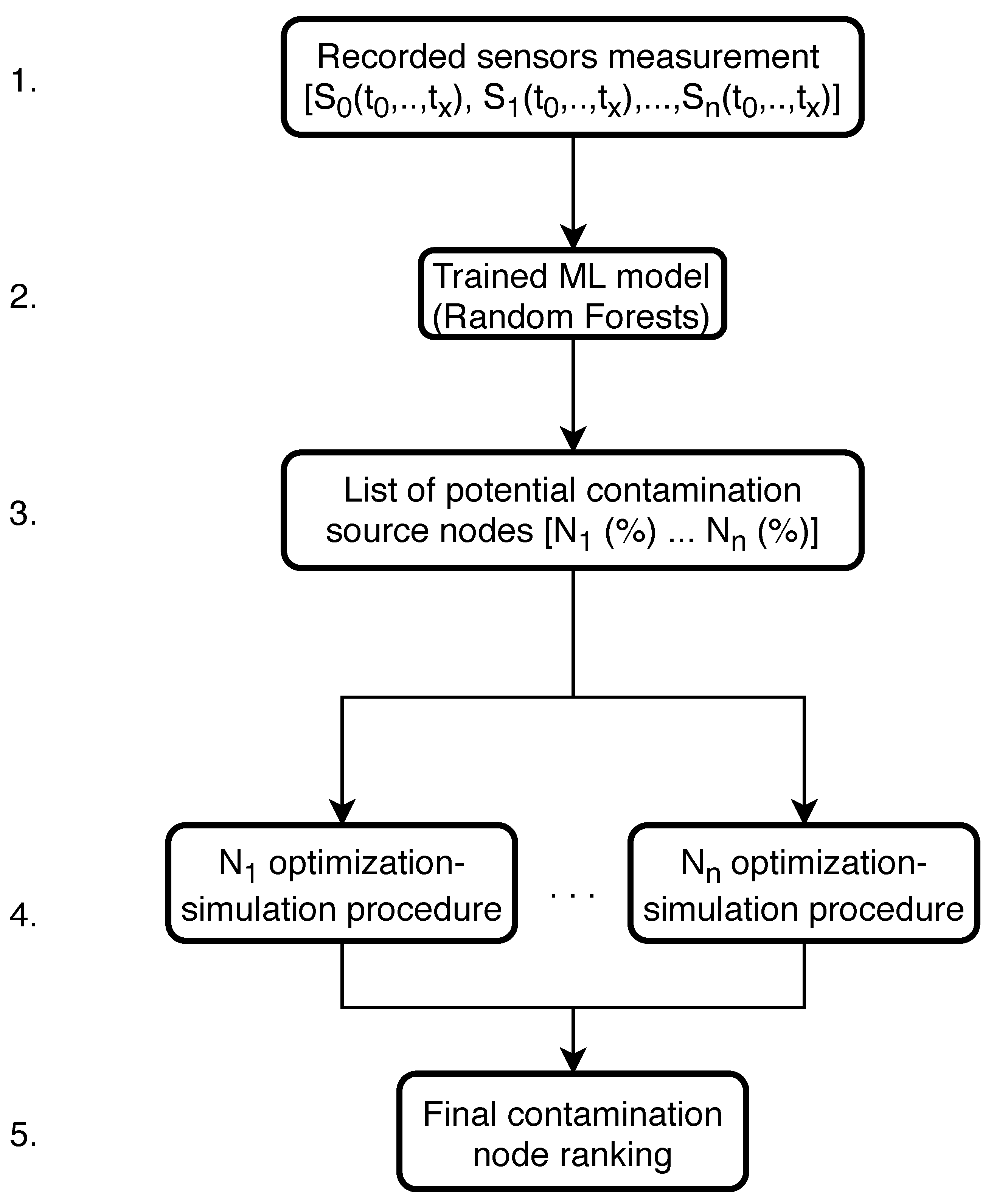
In this work, a novel methodology for predicting the water supply network contamination event is presented and investigated. Two algorithmic frameworks are constructed which are based on the methodology. Both frameworks utilize a machine learning approach based on the RF algorithm (implemented in the Python machine learning module scikit-learn 0.21.3 [43]) for potential contamination source search space reduction (as presented in our previous work [39]). The first investigated framework couples the simulation-optimization procedure directly with the RF classifier in order to determine the contamination start time, end time and injected contaminant concentration for each RF model predicted node separately and for this framework, three different stochastic optimization algorithms were investigated for one water distribution network benchmark. 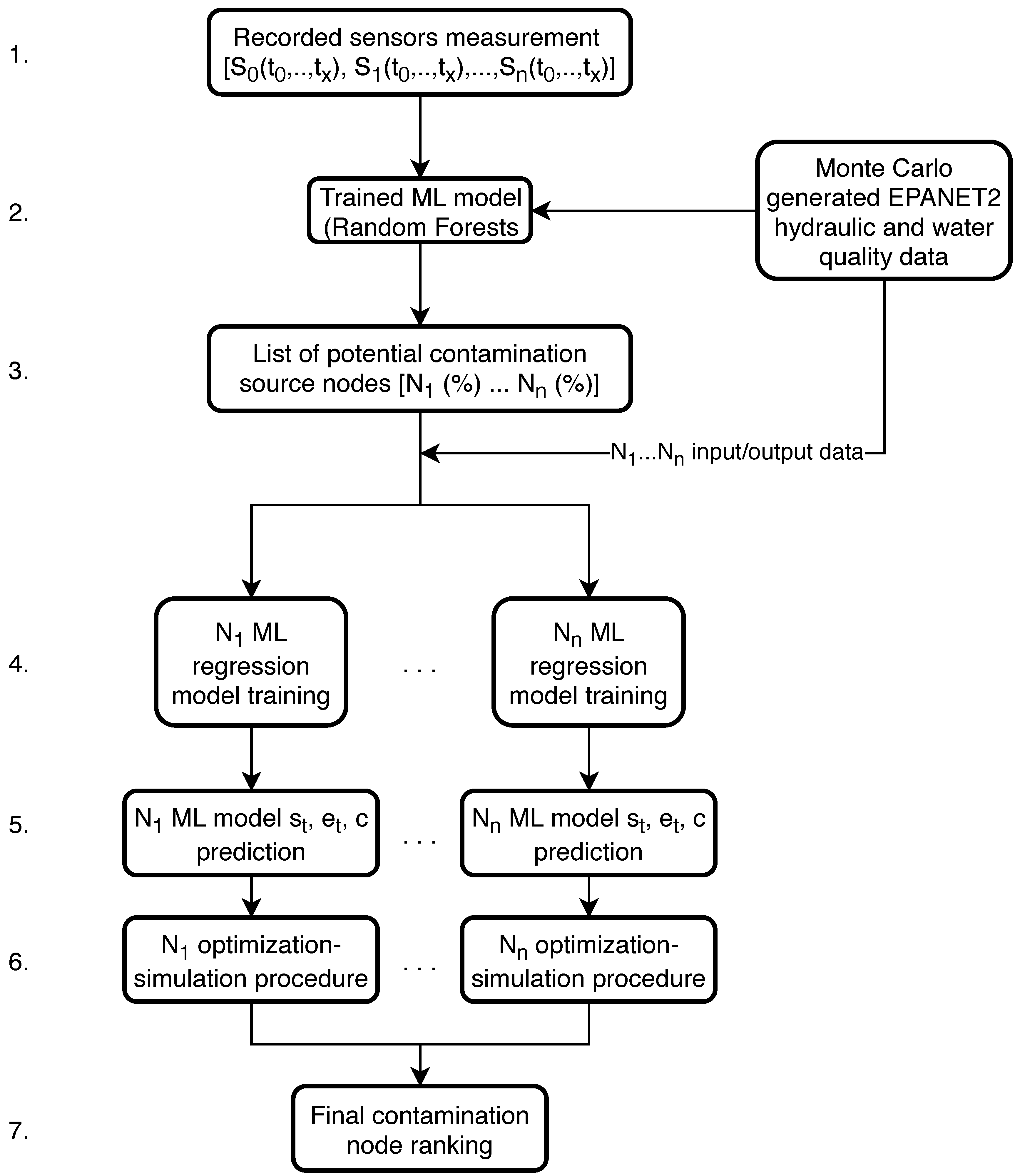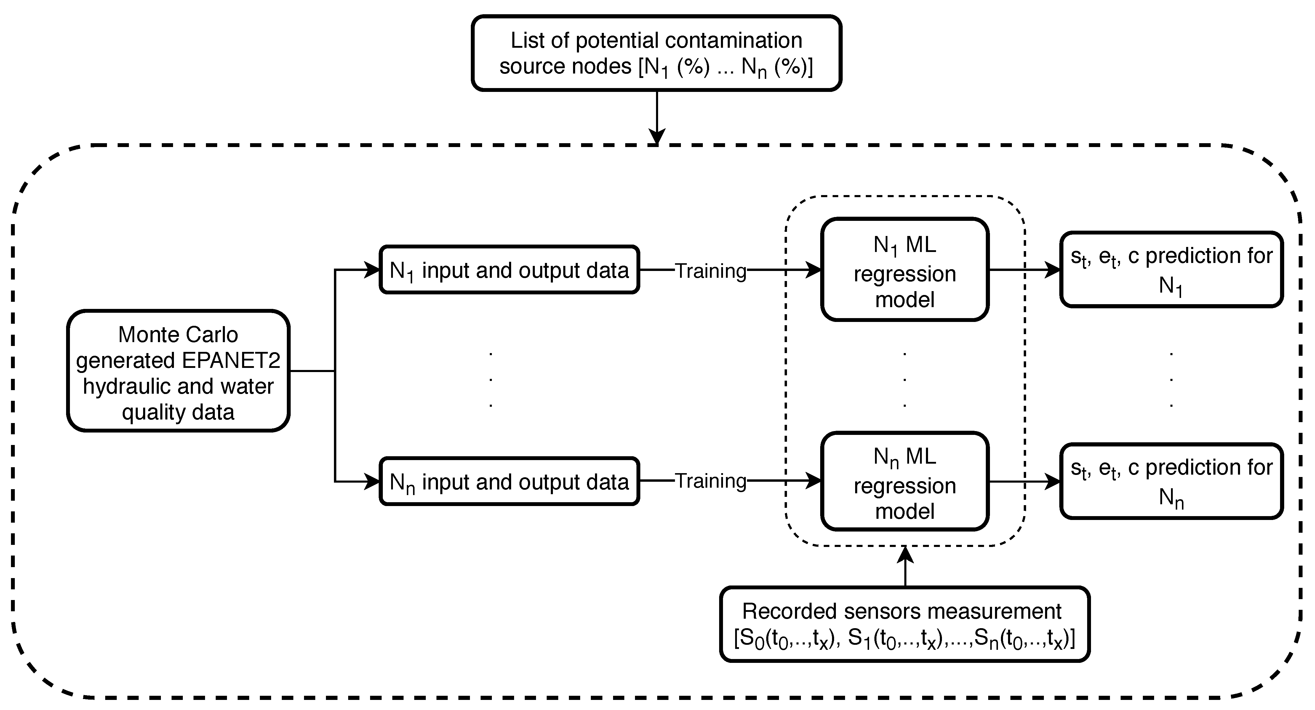The three stochastic optimization algorithms were Particle Swarm Optimization (PSO), fireworks algorithm (FWA), both implemented in the swarm optimization Python module indago 0.1.2 [44], and genetic algorithms (GA) implemented in the multiobjective optimization python module pymoo 0.4.2 [45]. The optimization algorithms were fine-tuned and the best performing one was further investigated with the coupling framework for both benchmark networks. The other algorithmic framework differs slightly as it includes an additional RF model regression for each RF predicted potential source node separately in order to predict each top node’s start time, end time and injected contaminant concentration. After the RF regression, each potential source node’s newly obtained data is then used as initial values for the deterministic global search optimization algorithm Mesh Adaptive Direct Search (MADS) which is implemented in NOMAD 4.0 [46].

The EPANET2 [3] hydraulic and water quality simulator is used for water supply network contamination event simulations. EPANET2 simulates contaminant transport using simplified complete mixing advection models which in most cases are not accurate enough as previously shown by [47]. However, for the purposes of examining the algorithm proposed in this study the simplified EPANET2 complete mixing model is good enough as the whole procedure is not dependent on the accuracy of the mixing processes occurring in the water distribution network. 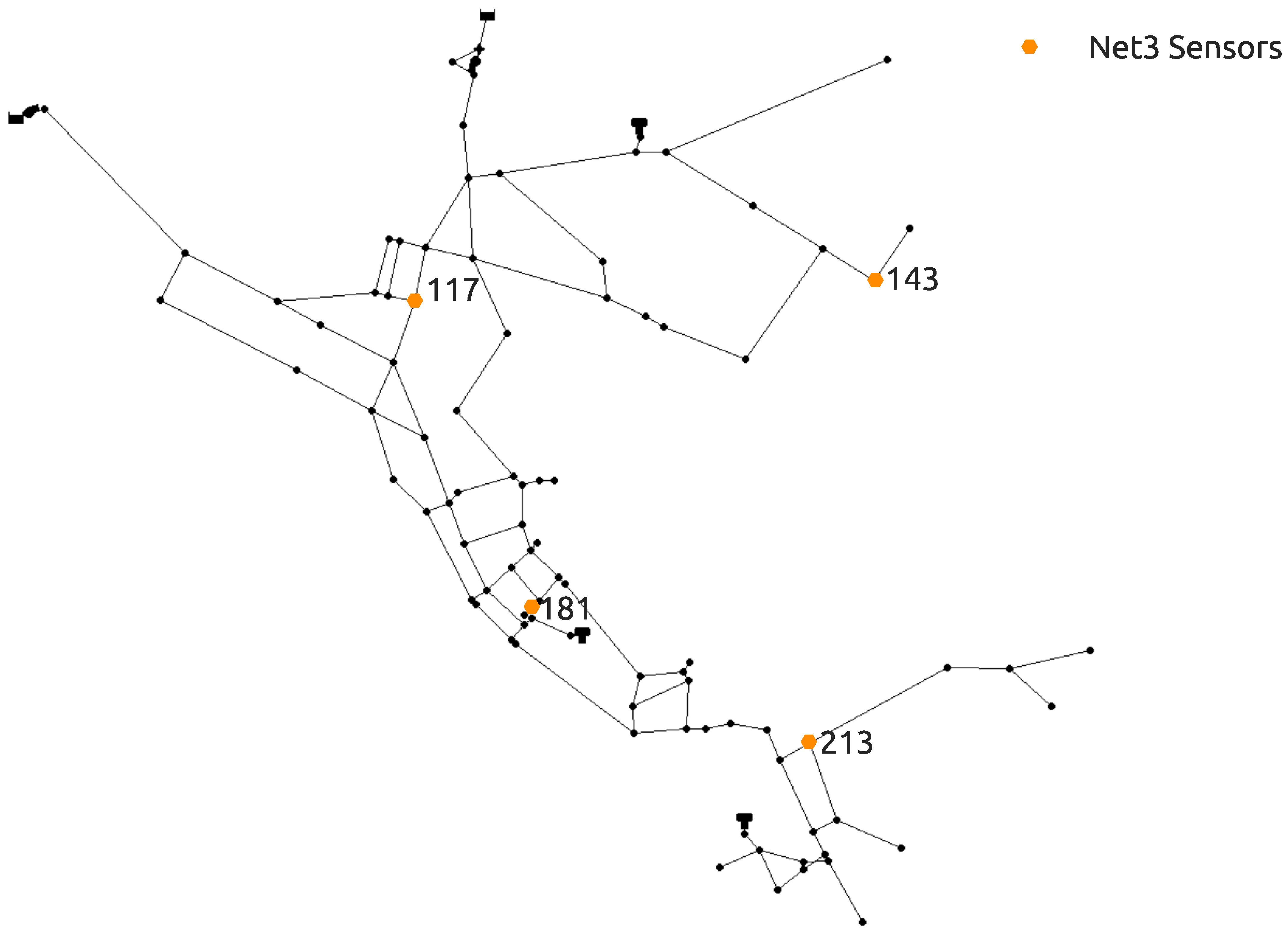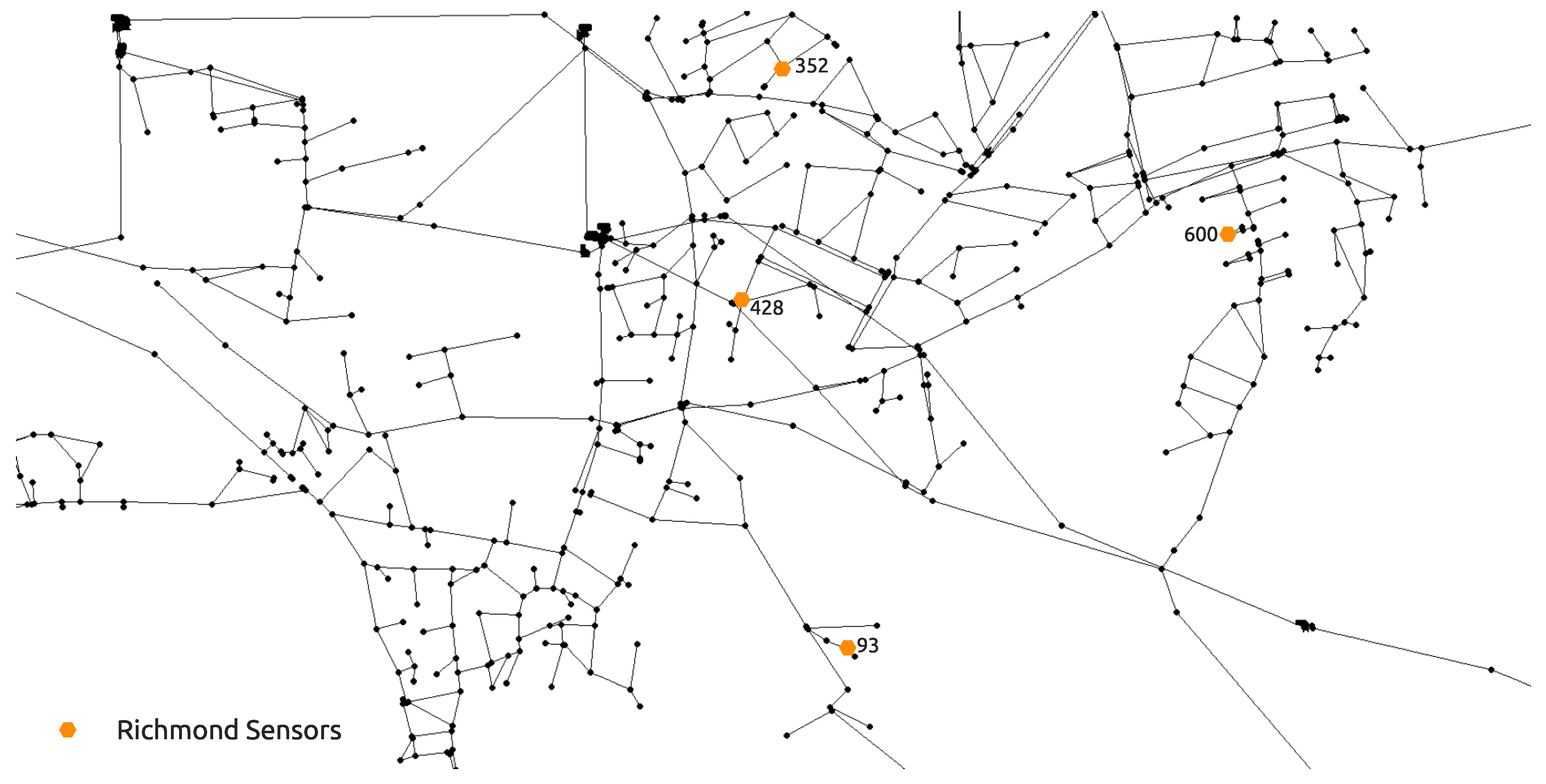Monte Carlo simulations are made to train the RF model for classification (as described in [39]) with the sensor water quality measurements being the input features and the true source node being the output. The RF model classifier then predicts the most probable contamination source nodes which are then submitted either to the stochastic simulation-optimization procedure (for the first framework) or to RF regression (trained with previously generated MC EPANET2 data) which predicts their start and end times and injected contaminant concentration. Both algorithmic frameworks are used on two water supply benchmark networks. The smaller benchmark network (92 nodes) was investigated with perfect sensor water quality measurements, while the bigger (865 nodes) was investigated with fuzzy sensor water quality measurements.

2. Materials and Methods

2.1. Water Distribution Network Benchmarks

The novel methodology was tested on two benchmark water distribution networks. The first benchmark is the NET3 EPANET2 water distribution network consisting of 92 total nodes which are all initially considered as potential source nodes. A 24 h period simulation time was set with a 1 h time step for the hydraulic analysis and a 5 min time step for the water quality analysis. A contamination pattern was set with a 10 min time step with all network sensors recording the quality of water every hour through the whole simulation (0–24 h). The injected contaminant is chemically or biologically unspecified and is treated as a mass which is introduced into the water distribution network since the investigated frameworks are independent of the transport model used in the simulation. The sensor positioning was the same as the one introduced in [48] and which showed in [39] to include a good number of suspect nodes when used in conjunction with the RF algorithm for classification. The NET3 water distribution network with the selected sensor layout can be seen in Figure 1. Since the total number of sensors is 4, a total of 100 water quality recordings were made through one simulation as each sensor detects the water quality in the network each hour for the 24 h interval (including the initial water quality at 00:00 h). The total hydraulic load or total demands of all nodes of the NET3 benchmark network through a 24 h simulation time interval can be observed in Figure 2.

The second, larger water distribution network used for the purposes of examining the proposed methodology is the hydraulically calibrated Richmond water distribution network introduced by [49] and it was downloaded from the Centre for Water Systems [50] benchmark repository. This benchmark water distribution network is located in Yorkshire, UK and covers an area which is 14 km wide and 3 km long. The larger network consists of 865 potential source nodes. For this case, the simulation time interval was 72 h and a hydraulic analysis time step of 1 h, water quality time step of 5 min and a contamination pattern step of 1 h which was only set in the first 24 h of the simulation. The sensor positioning proposed by [16] was used as it performs well with the RF classifier as shown in [39]. The total node demands of the NET3 benchmark network through a 72 h simulation time interval can be observed in Figure 3. The detail of the Richmond water distribution network is seen in Figure 4 which includes the positioning of 4 sensors, while the fifth sensor is located at node 672 (which is not seen in Figure 4 as it is outside the shown detail).

All five sensors of the Richmond network recorded the quality of water every hour for the period of 72 h which entails a total of 365 measurements (73 per sensor). Additionally, the sensor measurements were set as fuzzy (categorical) and not perfect as in the NET3 benchmark. This means that the measurements were not the true physical value of the contaminant but only a value which defines if the contamination is low, medium or high. If the measured injected contaminant concentration of the contaminant c was $0<c<100$ mg/L, the measured value was defined as low or 1; if it was $100\le c<500$ mg/L, it was defined as medium or 2; and if it was $c\ge 500$ mg/L, the value was considered high or 3. The fuzzy sensor measurements are used to investigate the algorithmic frameworks for a lower quality sensor technology.

2.2. Machine Learning and Simulation-Optimization Coupling Framework 1

The first algorithmic framework consists of machine learning classification of potential contamination source nodes which is then coupled with simulation-optimization procedure for each node separately in order to determine the contamination event start time $s_t$ (h), end time $e_t$ (h) and injected contaminant concentration c (mg/L) by minimizing the difference between the measured water quality sensor readings and the simulated water quality sensor readings with changing the initial conditions ($s_t$, $e_t$ and c) of the simulated contamination scenario.

Firstly, the machine learning model classifier was built the same way as in the work by [39] using Random Forests. The input variables for training the ML model were water supply network’s sensor measurements through a time interval ($S_0(t_0\dots t_x),S_1(t_0\dots t_x),\dots ,S_n(t_0\dots t_x)$, where $S_n$ is the n-th sensor in the network and $t_x$ is the water quality measurement at time step x) while the output was the true contamination source node for each sensor measurement. All data for the RF model training was generated with Monte Carlo EPANET2 hydraulic and water quality analysis where the source node N, $s_t$, $e_t$ and c were varied. If a water supply network contamination event were to occur, the sensor measurements would be submitted to the trained RF model classifier and a list of top potential source nodes would be generated.

The whole algorithmic framework of machine learning and simulation-optimization coupling can be observed in Figure 5. The procedure of water supply network contamination event reconstruction starts with inputting the recorded sensors measurements time series into the trained machine learning model (marked as 1. in Figure 5). The trained RF model (step 2.) generates a prediction of the most probable contamination source nodes based on the water supply network sensor measurements time series and compiles them in a list where each predicted node has a corresponding individual probability (%) of being the true contamination source node (step 3.).

The next step (4.) of the algorithmic framework is to separately submit each predicted potential source node to the simulation-optimization procedure. The optimization variables are $s_t$, $e_t$ and c and the goal function f of the simulation-optimization procedure is defined as:

$$f(s_t,e_t,c)=\sum _{i=0}^n\sum _{t=1}^T{(c_i^s\left(t\right)-c_i^m\left(t\right))}^2$$

(1)

where n is the number of water supply network sensors, T the simulation duration with a time step t, $c^m$ is the measured injected contaminant contaminant from the real contamination event and $c^s$ represents the simulated values of the contaminant. For the exact solution the goal function must yield zero for the true contamination source node.

When the simulation-optimization procedure is finished for each node, a final contamination node ranking is obtained (step 5.). The node with the smallest value of f (Equation (1)) can be considered the true contamination event source node. A problem can arise with the final source node ranking due to the strong multi-modal nature of the problem, which means that several potential source nodes can simultaneously converge to the same minimum value of f. The best performing stochastic optimization algorithm described in Section 2.5 was used for coupling with the ML classification.

2.3. Machine Learning and Simulation-Optimization Coupling Framework 2

This coupling framework differs slightly from the one described in Section 2.2. The general procedure is the same with an additional machine learning model regression added before the optimization algorithm with a to determine the values of $s_t$, $e_t$ and c using ML algorithms. Figure 6 shows the coupling framework.

Step 4. of the algorithmic framework is to separately train ML regression models for each predicted potential contamination source node (from steps 1.–3.) using pre-generated Monte Carlo data (EPANET2 hydraulic and water quality analysis) which was also used for the ML model classifier training (step 2.). This step is done in parallel where each node’s ML regression model is trained on a separate CPU. The input data of each node’s ML regression model training were the water supply network sensor measurements and the outputs were the corresponding values of $s_t$, $e_t$ and c. After each node’s ML regression models were trained, the recorded sensor measurements (from step 1.) were then used for prediction of $s_t$, $e_t$ and c (step 5.). Steps 4. and 5. of the algorithmic framework can be observed in Figure 7 with more detail.

Previously generated data by Monte Carlo simulations (which is also used to build the general ML classifier from step 2. in Figure 6 is used to build an individual node’s regression model. The input data for each node N are the simulated sensor readings ($S_0(t_0\dots t_x),S_1(t_0\dots t_x),\dots ,S_n(t_0\dots t_x)$) while the output data are the values of $s_t$, $e_t$ and c of each corresponding sensor reading. After the ML models are trained for all potential nodes (with all of the input and output data), the initial recorded sensor measurements are used as data inputs to generate each node’s predictions of $s_t$, $e_t$ and c. The Random Forest algorithm is also used for the machine learning regression in Step 4. as it was shown to work well for contamination source variables regression in the work by [37].

After each potential source node obtains a prediction of $s_t$, $e_t$ and c based on the recorded sensor measurements, the predicted values are passed to the next step (6.) of the framework. This step utilizes the simulation-optimization procedure for each node separately which entails that the only left optimization variables are continuous. Each node’s predicted values of $s_t$, $e_t$ and c are used as initial search values for a simulation-optimization procedure which utilizes a deterministic optimization algorithm. The goal function f of the simulation-optimization procedure is defined in Equation (1). The deterministic global search algorithm Mesh Adaptive Direct Search (MADS) was used in this coupling procedure and is described in Section 2.6.

2.4. Random Forests

Random Forests is an ensemble learning method used for classification and regression prediction [51,52]. The RF algorithm creates multiple decision trees that are defined with random feature selection (this process is also known as feature bootstrap aggregation or feature bagging). This is one of the strengths of the RF algorithm since with increased randomness of used features, the created decision trees have low variance and thus model overfitting is less likely to be a problem during the prediction process since there exists a de-correlation of each randomly constructed decision tree.

It was empirically shown that the RF algorithm outperforms the DT algorithm on multiple problems [53]. The generally most important RF algorithm training parameter is the used number of trees as the greater the number of trees is set, a more robust prediction will be achieved. The RF prediction process means that each randomly constructed decision tree creates its own prediction with the final decision or result being the most occurring one or rather the one with the most votes.

In the work by [54] the RF algorithm was compared other machine learning algorithms such as Logistic Regression, k-Nearest Neighbors, Support Vector Machine, Naive Bayes on a data classification problem regarding disease prediction and it showed better performance in accuracy. A recent review of RF algorithm applications specifically in the water resources applications filed is given by [55] where it was shown that is being increasingly utilized to build surrogate models. RF was used to enhance the low cost sensors performance for the purposes of air quality monitoring by [56] as the model’s prediction results were satisfactory when compared to empirical models. Additionally, [57] used RF in conjunction with remote sensing techniques for the purpose of dust source detection and mapping. It outperformed other machine learning algorithms such as Weights of Evidence (WOE) and Frequency Ratio (FR).

The RF implementation in the Python machine learning module scikit-learn 0.21.3. [43] was utilized for training the machine learning model for both algorithmic frameworks. The number of trees (the number of estimators) used for all RF models training in the algorithmic process was 250 while all of the other parameters were set as default. These settings were tuned with a grid search calibration of the RF model.

The $RandomForestClassifier$ and $RandomForestRegressor$ function from the scikit-learn 0.21.3 module $ensemble$ were used for classification and regression, respectively. For both functions the argument used was the number of estimators or trees. After object creation the functions $fit$ and $predict$ were used to train the RF model and predict the values of interest.

2.5. Stochastic Optimization Algorithms

2.5.1. Fireworks Algorithm

The fireworks optimization algorithm (FWA) is one of the investigated stochastic optimization algorithms in this study. It is a swarm intelligence algorithm generally used for optimization of complex goal functions and it is inspired by the process of fireworks explosions [58]. Ref. [59] created two frameworks for EEG signal data optimization which incorporated the single objective and multi objective FWA. In the work by [60] FWA was coupled with Evolutionary Computation for the purpose of classification and clustering on several different data sets. It was shown that it outperforms Particle Swarm Optimization for the same tasks.

The algorithm procedure includes randomly initializing a set of n fireworks for objective function evaluation with each of the n fireworks performing a local search through the search space. After each explosion a total number of explosion sparks $m_1$ are generated and the location of each explosion spark is obtained and evaluated. Better fireworks (in terms of fitness) will generate a greater number of sparks $m_1$ with a smaller amplitude of explosion while the ones with worse fitness values will contain a smaller number of sparks with a larger explosion amplitude. Additionally, a total of $m_2$ Gaussian mutated sparks are generated in order to increase diversity of the sparks. Every new generation of fireworks is constructed based on the fitness value, and both explosion sparks and the Gaussian mutated sparks. The FWA implementation in the python numerical optimization module indago 0.1.2 was used [44].

The indago 0.1.2. function $evaluation\_function$ was used to define the name of the optimization function, while the functions $dimensions$, $iterations$, $lb$, $ub$ and $params$ were used to define the number of optimization variables, iterations, lower bound, upper bound of the optimization problem and the optimization algorithm specific parameters, respectively. The $run$ function was used to start the optimization loop while f and X were minimum fitness and optimization variables at minimum fitness functions, respectively.

2.5.2. Particle Swarm Optimization

The second stochastic algorithm used in the preliminary analysis is the Particle Swarm Optimization (PSO) algorithm. PSO is a swarm intelligence algorithm inspired by the movement of birds [61]. A recent overview of the developments of PSO is given by [62]. PSO was used in the work by [63] for identifying the unknown groundwater contaminant sources as a part of the simulation-optimization procedure. In Ma et al. [64] PSO was used for gas emission source identification and compared with the firefly algorithm and Ant Colony Optimization algorithm. It was found that all of the three algorithms perform similarly in terms of estimating the source parameter but with PSO being computationally superior. In [65] PSO was used for the purpose of optimization of hydraulic demands of a water distribution network.

The particles which form a swarm with size s move through the objective search space with an inertia and are constantly both being attracted to the best position they have individually found and the best position determined by any other particle in the swarm. The parameters that influence the movement of each particle include the inertia factor w, cognitive and social factors $c_1$ and $c_2$. The languid particle dynamics modification [66] was used which involves setting the inertia of a particle to zero if it is not moving in the direction of better fitness. This modification was used as it proved beneficial to the standard PSO algorithm on the problem of water distribution pipe network routing [67]. The PSO implementation in the python numerical optimization module indago 0.1.2. was also used. The same indago functions were used as the one presented in the previous subsection but with different algorithm specific parameters set with the function $params$ since PSO was used.

2.5.3. Genetic Algorithms

The last examined stochastic algorithm is the genetic algorithm (GA) [68]. GA has been widely used in previous studies for the water network distribution contamination source detection problem [14,16]. A recent review of GA with a focus on the crossover and mutation rate choice was made by [69]. Recently, in the work by [70], GA was used to optimize a novel real-time control system for mitigation of sewer flooding and in [71] GA is implemented in an algorithmic procedure to investigate the wastewater seepage appearance in a semiarid urban environment.

GA is an algorithm inspired by the evolutionary process. A population (with size p) is formed by a set of individuals which are improved with each generation g. The formation of a new generation is based on the selection of the best performing individuals which is determined by their fitness value, the crossover parameter $c_r$ and the mutation m. The python module for multiobjective optimization pymoo 0.4.2. was used. The details and review of the specifics of the Python module pymoo can be found in the paper by the original authors [45].

The pymoo function $FunctionalProblem$ was used to define the whole optimization function which takes in as function arguments the number of optimization variables, the name of the predefined goal function and the lower and upper bounds of the optimization problem. The function $SingleObjectiveDefaultTermination$ was used to define the maximum number of generations as the stopping criterion. The mutation and crossover rates were defined with the functions $get\_mutation$ and $get\_crossover$. The mutation rate, crossover rate, population size were used as arguments for the genetic algorithm function $GA$ and finally, the optimization function, algorithm definition and the termination criterion were used as arguments for the pymoo $minimize$ function.

2.5.4. Preliminary Analysis

A preliminary analysis using the three different stochastic optimization algorithms was made and the best performing one was used for further investigation of the machine learning and simulation-optimization coupling framework 1. The preliminary analysis included finding the optimal solution or rather the values of $s_t$, $e_t$ and c for a known source node. The goal function was defined as in Equation (1) and the simulation-optimization procedure was done on the NET3 benchmark network with node 261 being the contamination source node. The true contamination event start time was 00:40 h, end time 06:30 and the injected contaminant concentration 78.5 mg/L. The optimization constraints for the start and end times were set as 00:00 h and 24:00 h (with a required condition that $s_t$ < $e_t$), while the injected contaminant concentration was bounded between 10 and. The contamination event parameters are summarized in

Table 1. NET3 network contamination event parameters.

Source Node	Start Time	End Time	Contaminant Concentration
261	00:40 h	06:30 h	78.5 mg/L

and the average contaminant mass flow which enters the node 261 can be observed in Figure 8. The maximum percentage of contamination mass thorough the time interval with relation to the total mass which passes through the true source node is 0.0078% for the proposed contamination event.

A parameter tuning process was also done for all of the three investigated algorithms through a grid search process. For each parameter combination of the three algorithms, a total of 100 repeated runs were made due to their stochastic nature. The performance was measured as the number of successful runs (cases in which all of the three optimization variables were predicted correctly with a fitness value below 0.02) out of 100 and the average time per run. A total of 256 parameter combinations were examined for each algorithm. The FWA varied values were iterations i, n, $m_1$ and $m_2$. For PSO the varied values were i, $c_1$, $c_2$ and the swarm size s and the GA varied values were g, p, $c_r$ and m. Summary of the results can be seen in

Table 2. Preliminary analysis of stochastic optimization algorithms—tuned parameters.

Algorithm	Successful Runs	Average Time per Run	Average f	Parameters
GA	100/100	121.5 s	0.015	g: 100, p: 80, $c_r$: 0.8, m: 0.1
PSO	98/100	178.6 s	0.003	i: 50, s: 100, $c_1$: 1, $c_2$: 1
FWA	100/100	64.13 s	0.009	i: 80, n: 5, $m_1$: 5, $m_2$: 10

. Out of the three algorithms, FWA has the best performance in terms of successful runs and the average time per run for the given parameters. The average value of the goal function f can also be seen in Table 2 with the lowest being achieved by PSO. FWA was used for further investigation of the coupling process within the algorithmic framework 1.

2.6. Deterministic Optimization Algorithm

Mesh Adaptive Direct Search

Mesh Adaptive Direct Search (MADS) was used as the deterministic optimization algorithm within the algorithmic framework 2 which includes the machine learning regression prediction model. MADS has not previously been used in research regarding water resources. In the recent work by [72] MADS optimization was used for the purposes autonomous vehicles control and in [73] it was successfully used to optimize the Gas-Lift procedure for maximizing the production of hydrocarbons from heavy oil and offshore reservoirs.

MADS is adequate for this kind of coupling as it must have an initial search condition which in this case is obtained from the RF regression (values of $s_t$, $e_t$ and c). MADS is an iterative method which includes creating a search space mesh for the optimization process [74]. The objective fitness search was achieved by mesh refinement within two essential steps—poll and search. The search step evaluates mesh points, and if progress of the fitness value is not achieved, a poll step performs a local search near the current best solution. If both steps do not find a better fitness value, the search space mesh is refined. The MADS implementation in the black box optimization open source software NOMAD 4.0 (developed at Polytechnique Montreal, Montreal, Canada) [46] was used. The only parameter used for the MADS optimization process was the number of goal function (Equation (1)) evaluations.

The NOMAD python wrapper PyNomad was used to form the optimization loop. The main NOMAD function used for evaluation is the $optimize$ function, which takes in as arguments the name of the optimization function; the initial search condition; lower optimization bound; upper bound; additional parameters $BB\_OUTPUT\_TYPEOBJ$ which define the output type (in this case the value of the objective function); and $MAX\_BB\_EVAL$, which is the maximum number of evaluations.

3. Results and Discussion

3.1. Random Forest Classifier Prediction

For both algorithmic frameworks and benchmark water distribution networks it is necessary to predict the top contamination source candidate nodes with the RF classifier. It is a requirement that the model is built before being employed in the algorithmic procedure. The whole process of training and prediction was repeated as in the work by [39].

The RF model classifier for the NET3 network was trained with 70,000 perfect sensor measurements (as input features) and true source nodes as the output features. The training and testing procedure lasted for 37 s on one INTEL E7 CPU core and an accuracy (30,000 input features) of 99% that the true source node was in the top 10 of the potential contamination source nodes predicted by the RF classifier was achieved. The trained classifier is then used within both coupling frameworks when NET3 network was investigated.

The same training process was repeated for the Richmond water distribution network with fuzzy sensor measurements as input features. Since the size of the network is larger that NET3 (865 potential source nodes), a total of 1,050,000 inputs were used for the RF model training and an accuracy of 99% was achieved for the true contamination source node being in the top 60 of the predicted potential source nodes. The training and testing process lasted for 955 s on the same hardware. A summary of both RF classifiers is given in

Table 3. Trained RF classifier characteristics.

Network	Sensors	Inputs	Top Nodes	Accuracy	Time
NET3	Perfect	70,000	10	99%	37 s
Richmond	Fuzzy	105,000	60	99%	955 s

.

3.2. Algorithmic Framework 1 Results

In this subsection the results of the coupling framework summarized in Section 2.2 are presented for both benchmark water distribution networks. All runs were done on one INTEL E7 node (manufactured by Intel Corporation, Santa Clara, CA, USA) with 256 cores. The FWA optimization algorithm is used with the tuned parameters specified in Section 2.5 for both networks.

The same NET3 contamination event parameters as presented in Table 1 were used to examine the efficiency and the robustness of the framework. The framework was repeatedly run for 100 times and for all runs the true source node (node 261) was in the top 10 of the potential source nodes predicted by the RF classifier and it was found in 99 out of 100 times after the simulation-optimization process had finished. After only one run, the selected contamination source node was node 263 as it is located closely to the true source node 261. This is a common occurrence in the contamination source detection procedure as the problem is greatly multimodal.

A summary of framework 1 results for the NET3 network can be observed in

Table 4. Framework 1 results for the NET3 network.

Run	Source Node	Start Time	End Time	Contaminant Concentration	f	Time
Average	261	0:39 h	6:29 h	78.49 mg/L	0.024	142 s
Most accurate	261	0:40 h	6:30 h	78.5 mg/L	0.002	133 s
Least accurate	263	0:20 h	6:20 h	78.7 mg/L	0.436	117 s

and it is shown that the algorithmic framework successfully determined the true source node contamination event parameters. The worst performing run is the one where the true source node was wrongly determined in terms while the best performing run has both the correct true source node and the best fitness. The values of average run correspond to the 99 runs when the true source node was node 261. In Figure 9 the sensor measurements of the contaminant through the 24 h period are shown. The least accurate result is the measurement for node 263 being the source node. It can be observed that the measurements between the most accurate and least accurate run differ greatly on sensor 143 (Figure 9b) while the measurement difference on other sensors in the network is minimal. The first coupling framework shows excellent convergence in a decent amount of time (average run was 142 s) for the NET3 benchmark network case with perfect sensor measurements.

The Richmond water distribution network contamination event parameters (start, end times and injected contaminant concentration with the network source node) can be seen in

Table 5. Richmond network contamination event parameters.

Source Node	Start Time	End Time	Contaminant Concentration
251	06:30 h	21:30 h	939.37 mg/L

. The coupling framework 1 was also repeatedly run 100 times for the Richmond network with the fuzzy sensor measurements. The average contaminant mass flow at the true source node 251 can be seen in Figure 10 and the maximum percentage of contamination mass over the simulation time is 0.0938% for this benchmark network case.

For 89 of 100 runs, the true source node was a tie in terms of fitness between two network nodes (node 251 and node 260). This is expected since as sensor measurements are not perfect and the multimodal nature of this problem is enhanced. For the remaining 11 runs, node 251 was selected to be the true source node for 4 runs while node 260 for seven runs. Both nodes are located closely to each other in the Richmond water distribution network and this can be seen in Figure 11 and in

Table 6. Framework 1 results for the Richmond network for the source node 251.

Run	Start Time	End Time	Contaminant Toncentration	f	Time
Average	6:30 h	21:00 h	940.6 mg/L	0.0	882 s
Most accurate	6:30 h	21:30 h	939.6 mg/L	0.0	852 s
Least accurate	6.30 h	11:40 h	943.9 mg/L	0.0	860 s

, a summary of the results for the true source node 251 is presented.

Interestingly, all of the 100 runs have the final fitness value of 0.0. This can be explained due to the simplicity of the fuzzy sensor measurements and the before mentioned enhanced multimodality of this problem where many solutions are equally as good in terms of the computed fitness. Due to the equally good fitness of all runs the accuracy of the results was determined with a root mean square error analysis of the contamination event parameters. The least accurate run severely underestimates the end time of the contamination event while all other parameters are predicted with good accuracy.

In

Table 7. Framework 1 results for the Richmond network for the source node 260.

Run	Start Time	End Time	Contaminant Concentration	f	Time
Average	6:30 h	20:09 h	915.6 mg/L	0.0	882 s
Most accurate	6:30 h	21:30 h	924.1 mg/L	0.0	843 s
Least accurate	6.30 h	14:50 h	908.4 mg/L	0.0	1002 s

, the results for the source node 260 can be observed. Even though the source location is wrong, the results are also useful due to the proximity of node 260 to the true source node and the good average prediction in terms of contamination event initial values.

3.3. Algorithmic Framework 2 Results

The second algorithmic framework which includes the ML regression model was also investigated for both benchmark networks with NET3 contamination event scenario parameters presented in Table 1 and Richmond parameters in Table 5. The number of iterations of the MADS algorithm was set to 300 for both water distribution benchmark network contamination event investigation. Framework 2 was also run for 100 times for both benchmark networks, as framework 1.

For the NET3 network the total number of Monte Carlo generated input data for the ML regression analysis (the whole procedure shown in Figure 7) was 300,000, which means each node’s regression model for a top 10 potential source node list had an average of 30,000 inputs. An analysis for the RF regression predicted values (for true source node 261) for a 300,000 total inputs can be seen in

Table 8. NET3 RF regression average values and standard deviations for 100 runs with absolute error.

	Average Prediction	Standard Deviation	Absolute Error
Start time	1:58 h	0:079 h	1:18 h
End time	6:56 h	0:15 h	0:16 h
Contaminant concentration	108.87 mg/L	5.17 mg/L	30.38 mg/L

. The RF regression is stable and robust as seen from the computed standard deviation of $s_t$, $e_t$ and c. The absolute error is the absolute distance from the contamination event parameters presented in Table 1 and it can be seen that the RF regression overestimates all of the three parameters, which is an additional proof that in order to reconstruct the whole contamination event scenario accurately, the simulation-optimization procedure is necessary.

In

Table 9. Framework 2 results for the NET3 network.

Run	Source Node	Start Time	End Time	Contaminant Concentration	f	Time
Average	261	0:31 h	6:30 h	78.48 mg/L	0.033	126 s
Most accurate	261	0:40 h	6:30 h	78.5 mg/L	0.002	124 s
Least accurate	261	0:00 h	6:30 h	78.2 mg/L	0.19	109 s

the framework 2 results for the NET3 benchmark network are presented. The true source node 261 was selected as the source node for all 100 runs. The average run time is about 20 s shorter than the average run time for framework 1 (as seen in Table 4). While the end time and injected contaminant concentration predictions are of great accuracy, the start time is slightly underestimated with an absolute error of 0.09 h. In Figure 12 the comparison of sensor measurements for the most accurate and the least accurate run of framework 2 can be observed and even though that the start time of the least accurate run has a 00:40 h absolute error, the measurements show to be very similar over the time interval than those presented in Figure 9 for framework 1. This is due to the contamination source node being wrongly selected in the least accurate run from framework 1, while for framework 2, all of the 100 runs were correct in terms of the source location.

For the Richmond water distribution network, the true source node (node 251) was selected in all of the 100 runs. For 63 of the 100 runs the true source node was the only selected node of the framework while for the remaining 37 runs it was a tie between node 251 and 260. The total number of input data for the RF regression procedure was 785,000. The analysis of the RF predicted values (for true source node 251) can be seen in

Table 10. Richmond RF regression average values and standard deviations for 100 runs with an absolute error.

	Average Prediction	Standard Deviation	Absolute Error
Start time	6:53 h	0:015 h	0:28 h
End time	17:57 h	0:049 h	3:73 h
Contaminant concentration	933.97 mg/L	0.96 mg/L	5.4 mg/L

. The standard deviation for all three values is small which means that the RF prediction is robust while the absolute error is the biggest for the end time prediction.

Table 11. Framework 2 results for the Richmond network for the source node 251.

Run	Start Time	End Time	Contaminant Concentration	f	Time
Average	6:30 h	22:22 h	942.2 mg/L	0.0	632.7 s
Most accurate	6:30 h	21:30 h	939.7 mg/L	0.0	602 s
Least accurate	6.30 h	22:20 h	944.3 mg/L	0.0	591 s

and

Table 12. Framework 2 results for the Richmond network for the source node 260.

Run	Start Time	End Time	Contaminant Concentration	f	Time
Average	6:30 h	15:73 h	917.8 mg/L	0.0	632.7 s
Most accurate	6:30 h	17:40 h	924.3 mg/L	0.0	570 s
Least accurate	6.30 h	15:40 h	908.5 mg/L	0.0	596 s

show the results of 100 runs for the predicted source nodes. The average start time and the injected contaminant concentration are quite accurately predicted for the source node 251 while the end time of the contamination event scenario is slightly overestimated. Nonetheless, framework 2 with the MADS algorithm exhibits great robustness in determining the true source node as it was selected 63 out of 100 times as the only source node.

3.4. Framework Comparison

Both frameworks presented in this study have shown robustness and good accuracy in determining the contamination source node and parameters of the contamination event. Framework 1 has shown to be more accurate than framework 2 in determining the values of $s_t$, $e_t$ and c for both benchmark networks when the average values of 100 repeated runs are observed, however framework 2 has shown to obtain good results in less time. The greatest benefit of framework 2 which includes the RF regression model is that it is extremely robust in determining the true source node for the fuzzy sensor measurements benchmark example as it outperformed framework 1. In

Table 13. A comparison of frameworks 1 and 2 in determining the true source node for both network benchmarks.

Framework	Network	Runs	True Source	False Source	Tie
1	NET3	100	99	1	0
2	NET3	100	100	0	0
1	Richmond	100	4	7	89
2	Richmond	100	63	0	37

the true source node detection comparison for the two presented frameworks is given.

4. Conclusions

In this study two algorithmic frameworks for water distribution network contamination event detection were presented. Both frameworks were tested on a small water distribution benchmark network with 92 potential sources with perfect sensor measurements and a bigger benchmark network with 865 potential sources which included fuzzy sensor measurements to examine the robustness of the frameworks.

The first algorithmic framework includes coupling a ML classification model based on the RF algorithm and a stochastic optimization algorithm. After a preliminary analysis and parameters calibration procedure on the smaller benchmark network, the fireworks algorithm showed to be superior to the Particle Swarm Optimization algorithm and the genetic algorithms which are the most popular optimization algorithms for the water network contamination source detection problem. The algorithmic framework with the Fireworks algorithm shows to work with good accuracy in predicting the start time, end time and injected contaminant concentration for both benchmark networks but lacks the robustness of predicting the true source node with fuzzy sensor measurements.

The second presented algorithmic framework has an added ML regression model for each of the potential source nodes generated by the RF classifier. The regression model is trained pre-generated data by Monte Carlo simulations in parallel. The framework was coupled with the Mesh Adaptive Direct Search algorithm which is extremely well suited for this procedure as it requires an initial search value which in this case is generated by the RF regression model. This framework showed to be robust and can predict with good accuracy the true source node when the contamination event incorporates fuzzy measurements.

The proposed methodology differs from other methods for contamination source node identification, as it combines the two more general approaches in a whole framework. Usually the simulation-optimization methods and data-driven machine learning based methods are uncoupled and used separately for the task of contamination source detection. With this approach, the strength of identifying the most probable source nodes via a machine learning algorithm is coupled with the strength of finding the start time, end time and injected contaminant concentration through simulation-optimization algorithms. The proposed methodology is computationally efficient since a search space reduction is achieved with the machine learning approach.

Hydraulic demand uncertainties of the water distribution networks should be included in future studies as they were not investigated with this framework, but as shown in [39], the RF classifier accuracy is slightly lowered when they are incorporated. In future studies other ML algorithms could be tested for the classification part of both algorithmic frameworks and the regression part of the second framework. Additionally, other optimization algorithms (stochastic and deterministic) could also be incorporated into both algorithmic frameworks and investigated.

References

1. Ng, D.Q.; Chen, C.Y.; Lin, Y.P. A new scenario of lead contamination in potable water distribution systems: Galvanic corrosion between lead and stainless steel. Sci. Total Environ. 2018, 637, 1423–1431. [Google Scholar] [CrossRef]
2. Inkinen, J.; Kaunisto, T.; Pursiainen, A.; Miettinen, I.T.; Kusnetsov, J.; Riihinen, K.; Keinänen-Toivola, M.M. Drinking water quality and formation of biofilms in an office building during its first year of operation, a full scale study. Water Res. 2014, 49, 83–91. [Google Scholar] [CrossRef] [PubMed]
3. Rossman, L.A. EPANET 2: Users Manual; US Environmental Protection Agency, Office of Research and Development: Washington, DC, USA, 2000. [Google Scholar]
4. Ostfeld, A.; Uber, J.G.; Salomons, E.; Berry, J.W.; Hart, W.E.; Phillips, C.A.; Watson, J.P.; Dorini, G.; Jonkergouw, P.; Kapelan, Z.; et al. The battle of the water sensor networks (BWSN): A design challenge for engineers and algorithms. J. Water Resour. Plan. Manag. 2008, 134, 556–568. [Google Scholar] [CrossRef] [Green Version]
5. Ung, H.; Piller, O.; Gilbert, D.; Mortazavi, I. Accurate and Optimal Sensor Placement for Source Identification of Water Distribution Networks. J. Water Resour. Plan. Manag. 2017, 143, 04017032. [Google Scholar] [CrossRef] [Green Version]
6. Hooshmand, F.; Amerehi, F.; MirHassani, S. Risk-Based Models for Optimal Sensor Location Problems in Water Networks. J. Water Resour. Plan. Manag. 2020, 146, 04020086. [Google Scholar] [CrossRef]
7. Santonastaso, G.F.; Di Nardo, A.; Creaco, E.; Musmarra, D.; Greco, R. Comparison of topological, empirical and optimization-based approaches for locating quality detection points in water distribution networks. Environ. Sci. Pollut. Res. 2020, 1–10. [Google Scholar] [CrossRef]
8. Alfonso, L.; Jonoski, A.; Solomatine, D. Multiobjective optimization of operational responses for contaminant flushing in water distribution networks. J. Water Resour. Plan. Manag. 2010, 136, 48–58. [Google Scholar] [CrossRef]
9. Hu, C.; Yan, X.; Gong, W.; Liu, X.; Wang, L.; Gao, L. Multi-objective based scheduling algorithm for sudden drinking water contamination incident. Swarm Evol. Comput. 2020, 55, 100674. [Google Scholar] [CrossRef]
10. Khaksar Fasaee, M.A.; Nikoo, M.R.; Hashempour Bakhtiari, P.; Monghasemi, S.; Sadegh, M. A novel dynamic hydrant flushing framework facilitated by categorizing contamination events. Urban Water J. 2020, 1–13. [Google Scholar] [CrossRef]
11. Kranjčević, L.; Čavrak, M.; Šestan, M. Contamination source detection in water distribution networks. Eng. Rev. 2010, 30, 11–25. [Google Scholar]
12. Xuesong, Y.; Jie, S.; Chengyu, H. Research on contaminant sources identification of uncertainty water demand using genetic algorithm. Clust. Comput. 2017, 20, 1007–1016. [Google Scholar] [CrossRef]
13. Yan, X.; Zhu, Z.; Li, T. Pollution source localization in an urban water supply network based on dynamic water demand. Environ. Sci. Pollut. Res. 2019, 26, 17901–17910. [Google Scholar] [CrossRef]
14. Adedoja, O.; Hamam, Y.; Khalaf, B.; Sadiku, R. Towards development of an optimization model to identify contamination source in a water distribution network. Water 2018, 10, 579. [Google Scholar] [CrossRef] [Green Version]
15. Berglund, E.Z.; Pesantez, J.E.; Rasekh, A.; Shafiee, M.E.; Sela, L.; Haxton, T. Review of Modeling Methodologies for Managing Water Distribution Security. J. Water Resour. Plan. Manag. 2020, 146, 03120001. [Google Scholar] [CrossRef]
16. Preis, A.; Ostfeld, A. Genetic algorithm for contaminant source characterization using imperfect sensors. Civ. Eng. Environ. Syst. 2008, 25, 29–39. [Google Scholar] [CrossRef]
17. Yan, X.; Zhao, J.; Hu, C.; Zeng, D. Multimodal optimization problem in contamination source determination of water supply networks. Swarm Evol. Comput. 2019, 47, 66–71. [Google Scholar] [CrossRef]
18. Hu, C.; Zhao, J.; Yan, X.; Zeng, D.; Guo, S. A MapReduce based Parallel Niche Genetic Algorithm for contaminant source identification in water distribution network. Ad Hoc Netw. 2015, 35, 116–126. [Google Scholar] [CrossRef]
19. Vankayala, P.; Sankarasubramanian, A.; Ranjithan, S.R.; Mahinthakumar, G. Contaminant source identification in water distribution networks under conditions of demand uncertainty. Environ. Forensics 2009, 10, 253–263. [Google Scholar] [CrossRef]
20. Yan, X.; Gong, J.; Wu, Q. Pollution source intelligent location algorithm in water quality sensor networks. Neural Comput. Appl. 2020, 33, 209–222. [Google Scholar] [CrossRef]
21. Liu, L.; Zechman, E.M.; Mahinthakumar, G.; Ranjithan, S.R. Coupling of logistic regression analysis and local search methods for characterization of water distribution system contaminant source. Eng. Appl. Artif. Intell. 2012, 25, 309–316. [Google Scholar] [CrossRef]
22. Lučin, I.; Grbčić, L.; Družeta, S.; Čarija, Z. Source Contamination Detection Using Novel Search Space Reduction Coupled with Optimization Technique. J. Water Resour. Plan. Manag. 2020, 147, 04020100. [Google Scholar] [CrossRef]
23. Yan, X.; Zhao, J.; Hu, C. Research on multimodal optimization algorithm for the contamination source identification of city water distribution networks. In International Conference on Bio-Inspired Computing: Theories and Applications; Springer: Berlin/Heidelberg, Germany, 2016; pp. 80–85. [Google Scholar]
24. Yan, X.; Gong, W.; Wu, Q. Contaminant source identification of water distribution networks using cultural algorithm. Concurr. Comput. Pract. Exp. 2017, 29, e4230. [Google Scholar] [CrossRef]
25. Yan, X.; Zhao, J.; Hu, C.; Wu, Q. Contaminant source identification in water distribution network based on hybrid encoding. J. Comput. Methods Sci. Eng. 2016, 16, 379–390. [Google Scholar] [CrossRef]
26. Yan, X.; Hu, C.; Sheng, V.S. Data-driven pollution source location algorithm in water quality monitoring sensor networks. Int. J. Bio-Inspired Comput. 2020, 15, 171–180. [Google Scholar] [CrossRef]
27. Park, Y.J.; Tagade, P.M.; Choi, H.L. Deep gaussian process-based bayesian inference for contaminant source localization. IEEE Access 2018, 6, 49432–49449. [Google Scholar] [CrossRef]
28. Wang, C.; Zhou, S. Contamination source identification based on sequential Bayesian approach for water distribution network with stochastic demands. IISE Trans. 2017, 49, 899–910. [Google Scholar] [CrossRef]
29. Sankary, N.; Ostfeld, A. Bayesian localization of water distribution system contamination intrusion events using inline mobile sensor data. J. Water Resour. Plan. Manag. 2019, 145, 04019029. [Google Scholar] [CrossRef]
30. Gong, J.; Yan, X.; Chengyu, H.; Qinghua, W. Collaborative based pollution sources identification algorithm in water supply sensor networks. Desalination Water Treat. 2019, 168, 123–135. [Google Scholar] [CrossRef]
31. Le, X.H.; Ho, H.V.; Lee, G.; Jung, S. Application of long short-term memory (LSTM) neural network for flood forecasting. Water 2019, 11, 1387. [Google Scholar] [CrossRef] [Green Version]
32. Cho, J.; Kim, H.; Gebreselassie, A.L.; Shin, D. Deep neural network and random forest classifier for source tracking of chemical leaks using fence monitoring data. J. Loss Prev. Process Ind. 2018, 56, 548–558. [Google Scholar] [CrossRef]
33. Zhou, Z.; Tartakovsky, D.M. Markov chain Monte Carlo with neural network surrogates: Application to contaminant source identification. Stoch. Environ. Res. Risk Assess. 2020, 1–13. [Google Scholar] [CrossRef]
34. Kim, M.; Choi, C.Y.; Gerba, C.P. Source tracking of microbial intrusion in water systems using artificial neural networks. Water Res. 2008, 42, 1308–1314. [Google Scholar] [CrossRef] [PubMed] [Green Version]
35. Rutkowski, T.; Prokopiuk, F. Identification of the Contamination Source Location in the Drinking Water Distribution System Based on the Neural Network Classifier. IFAC-PapersOnLine 2018, 51, 15–22. [Google Scholar] [CrossRef]
36. Sun, L.; Yan, H.; Xin, K.; Tao, T. Contamination source identification in water distribution networks using convolutional neural network. Environ. Sci. Pollut. Res. 2019, 26, 36786–36797. [Google Scholar] [CrossRef]
37. Grbčić, L.; Lučin, I.; Kranjčević, L.; Družeta, S. A Machine Learning-based Algorithm for Water Network Contamination Source Localization. Sensors 2020, 20, 2613. [Google Scholar] [CrossRef]
38. Eliades, D.G.; Polycarpou, M.M. Water contamination impact evaluation and source-area isolation using decision trees. J. Water Resour. Plan. Manag. 2011, 138, 562–570. [Google Scholar] [CrossRef]
39. Grbčić, L.; Lučin, I.; Kranjčević, L.; Družeta, S. Water supply network pollution source identification by random forest algorithm. J. Hydroinform. 2020. [Google Scholar] [CrossRef]
40. Lučin, I.; Grbčić, L.; Čarija, Z.; Kranjčević, L. Machine-Learning Classification of a Number of Contaminant Sources in an Urban Water Network. Sensors 2021, 21, 245. [Google Scholar] [CrossRef] [PubMed]
41. Lee, Y.J.; Park, C.; Lee, M.L. Identification of a contaminant source location in a river system using random forest models. Water 2018, 10, 391. [Google Scholar] [CrossRef] [Green Version]
42. Bashi-Azghadi, S.N.; Kerachian, R.; Bazargan-Lari, M.R.; Solouki, K. Characterizing an unknown pollution source in groundwater resources systems using PSVM and PNN. Expert Syst. Appl. 2010, 37, 7154–7161. [Google Scholar] [CrossRef]
43. Pedregosa, F.; Varoquaux, G.; Gramfort, A.; Michel, V.; Thirion, B.; Grisel, O.; Blondel, M.; Prettenhofer, P.; Weiss, R.; Dubourg, V.; et al. Scikit-learn: Machine learning in Python. J. Mach. Learn. Res. 2011, 12, 2825–2830. [Google Scholar]
44. Družeta, S.; Ivić, S. Indago—Python Module for Numerical Optimization. Available online: https://pypi.org/project/Indago/ (accessed on 10 September 2020).
45. Blank, J.; Deb, K. pymoo: Multi-objective Optimization in Python. IEEE Access 2020, 8, 89497–89509. [Google Scholar] [CrossRef]
46. Audet, C.; Le Digabel, S.; Tribes, C. NOMAD User Guide; Technical Report G-2009-37, Les cahiers du GERAD; Polytechnique Montreal: Montreal, QC, Canada , 2009. [Google Scholar]
47. Piazza, S.; Blokker, E.M.; Freni, G.; Puleo, V.; Sambito, M. Impact of diffusion and dispersion of contaminants in water distribution networks modelling and monitoring. Water Supply 2020, 20, 46–58. [Google Scholar] [CrossRef]
48. Preis, A.; Ostfeld, A. A contamination source identification model for water distribution system security. Eng. Optim. 2007, 39, 941–947. [Google Scholar] [CrossRef]
49. Van Zyl, J.E. A Methodology for Improved Operational Optimization of Water Distribution Systems. Ph.D Thesis, University of Exeter UK, Exeter, UK, 2001. [Google Scholar]
50. CWS, U.o.E. CWS Benchmarks. Available online: http://emps.exeter.ac.uk/engineering/research/cws/downloads/benchmarks/ (accessed on 6 November 2019).
51. Ho, T.K. Random decision forests. In Proceedings of the 3rd International Conference on Document Analysis and Recognition, Montreal, QC, Canada, 14–16 August 1995; Volume 1, pp. 278–282. [Google Scholar]
52. Breiman, L. Random forests. Mach. Learn. 2001, 45, 5–32. [Google Scholar] [CrossRef] [Green Version]
53. Caruana, R.; Niculescu-Mizil, A. An empirical comparison of supervised learning algorithms. In Proceedings of the 23rd International Conference on Machine Learning, Pittsburgh, PA, USA, 25–29 June 2006; pp. 161–168. [Google Scholar]
54. Hassan, C.A.U.; Khan, M.S.; Shah, M.A. Comparison of Machine Learning Algorithms in Data classification. In Proceedings of the 2018 24th International Conference on Automation and Computing (ICAC), Newcastle upon Tyne, UK, 6–7 September 2018; pp. 1–6. [Google Scholar]
55. Tyralis, H.; Papacharalampous, G.; Langousis, A. A brief review of random forests for water scientists and practitioners and their recent history in water resources. Water 2019, 11, 910. [Google Scholar] [CrossRef] [Green Version]
56. Zimmerman, N.; Presto, A.A.; Kumar, S.P.; Gu, J.; Hauryliuk, A.; Robinson, E.S.; Robinson, A.L.; Subramanian, R. A machine learning calibration model using random forests to improve sensor performance for lower-cost air quality monitoring. Atmos. Meas. Tech. 2018, 11, 291–313. [Google Scholar] [CrossRef] [Green Version]
57. Boroughani, M.; Pourhashemi, S.; Hashemi, H.; Salehi, M.; Amirahmadi, A.; Asadi, M.A.Z.; Berndtsson, R. Application of remote sensing techniques and machine learning algorithms in dust source detection and dust source susceptibility mapping. Ecol. Inform. 2020, 56, 101059. [Google Scholar] [CrossRef]
58. Tan, Y.; Zhu, Y. Fireworks algorithm for optimization. In International Conference in Swarm Intelligence; Springer: Berlin/Heidelberg, Germany, 2010; pp. 355–364. [Google Scholar]
59. El Majdouli, M.A.; Rbouh, I.; Bougrine, S.; El Benani, B.; El Imrani, A.A. Fireworks algorithm framework for Big Data optimization. Memetic Comput. 2016, 8, 333–347. [Google Scholar] [CrossRef]
60. Xue, Y.; Zhao, B.; Ma, T.; Liu, A.X. An evolutionary classification method based on fireworks algorithm. Int. J. Bio-Inspired Comput. 2018, 11, 149–158. [Google Scholar] [CrossRef]
61. Kennedy, J.; Eberhart, R. Particle swarm optimization. In Proceedings of the ICNN’95-International Conference on Neural Networks; IEEE: New York, NY, USA, 1995; Volume 4, pp. 1942–1948. [Google Scholar]
62. Wang, D.; Tan, D.; Liu, L. Particle swarm optimization algorithm: An overview. Soft Comput. 2018, 22, 387–408. [Google Scholar] [CrossRef]
63. Guneshwor, L.; Eldho, T.; Kumar, A.V. Identification of groundwater contamination sources using meshfree RPCM simulation and particle swarm optimization. Water Resour. Manag. 2018, 32, 1517–1538. [Google Scholar] [CrossRef]
64. Ma, D.; Tan, W.; Wang, Q.; Zhang, Z.; Gao, J.; Zeng, Q.; Wang, X.; Xia, F.; Shi, X. Application and improvement of swarm intelligence optimization algorithm in gas emission source identification in atmosphere. J. Loss Prev. Process Ind. 2018, 56, 262–271. [Google Scholar] [CrossRef]
65. Letting, L.K.; Hamam, Y.; Abu-Mahfouz, A.M. Estimation of water demand in water distribution systems using particle swarm optimization. Water 2017, 9, 593. [Google Scholar] [CrossRef] [Green Version]
66. Družeta, S.; Ivić, S. Examination of benefits of personal fitness improvement dependent inertia for Particle Swarm Optimization. Soft Comput. 2017, 21, 3387–3400. [Google Scholar] [CrossRef]
67. Družeta, S.; Ivić, S.; Grbčić, L.; Lučin, I. Introducing languid particle dynamics to a selection of PSO variants. Egypt. Inform. J. 2020, 21, 119–129. [Google Scholar] [CrossRef]
68. Holland, J.H. Genetic algorithms. Sci. Am. 1992, 267, 66–73. [Google Scholar] [CrossRef]
69. Hassanat, A.; Almohammadi, K.; Alkafaween, E.; Abunawas, E.; Hammouri, A.; Prasath, V. Choosing mutation and crossover ratios for genetic algorithms—A review with a new dynamic approach. Information 2019, 10, 390. [Google Scholar] [CrossRef] [Green Version]
70. Mounce, S.; Shepherd, W.; Ostojin, S.; Abdel-Aal, M.; Schellart, A.; Shucksmith, J.; Tait, S. Optimisation of a fuzzy logic-based local real-time control system for mitigation of sewer flooding using genetic algorithms. J. Hydroinform. 2020, 22, 281–295. [Google Scholar] [CrossRef]
71. Attwa, M.; Zamzam, S. An integrated approach of GIS and geoelectrical techniques for wastewater leakage investigations: Active constraint balancing and genetic algorithms application. J. Appl. Geophys. 2020, 175, 103992. [Google Scholar] [CrossRef]
72. Naranjo, J.E.; Serradilla, F.; Nashashibi, F. Speed Control Optimization for Autonomous Vehicles with Metaheuristics. Electronics 2020, 9, 551. [Google Scholar] [CrossRef] [Green Version]
73. Khoshkbarchi, M.; Rahmanian, M.; Cordazzo, J.; Nghiem, L. Application of Mesh Adaptive Derivative-Free Optimization Technique for Gas-Lift Optimization in an Integrated Reservoirs, Wells, and Facilities Modeling Environment. In Proceedings of the Society of Petroleum Engineers SPE/Canada Heavy Oil Conference, Virtual Conference. 28 September–2 October 2020. [Google Scholar]
74. Audet, C.; Dennis, J.E., Jr. Mesh adaptive direct search algorithms for constrained optimization. SIAM J. Optim. 2006, 17, 188–217. [Google Scholar] [CrossRef] [Green Version]
Figure 1. NET3 water distribution network benchmark with sensor positioning.
Sensors 21 01157 g001
Figure 2. NET3 water distribution network total hydraulic demands over a 24 h period.
Sensors 21 01157 g002
Figure 3. Richmond water distribution network total hydraulic demands over a 72 h period.
Sensors 21 01157 g003
Figure 4. Richmond water distribution network benchmark detail with the positions of 4 sensors.
Sensors 21 01157 g004
Figure 5. Machine learning and simulation-optimization coupling algorithmic framework 1 flowchart.
Sensors 21 01157 g005
Figure 6. Machine learning and simulation-optimization coupling algorithmic framework 2 flowchart.
Sensors 21 01157 g006
Figure 7. Machine learning regression model flowchart.
Sensors 21 01157 g007
Figure 8. Average contaminant mass flow at the source node 261 over a 24 h period.
Sensors 21 01157 g008
Figure 9. A comparison of sensor measurements through time for the NET3 benchmark network (framework 1).
Sensors 21 01157 g009
Figure 10. Average contaminant mass flow at the source node 251 for the Richmond network over a 72 h period.
Sensors 21 01157 g010
Figure 11. Network node locations of the two top candidate source nodes 251 and 260 (zoomed in part of the network).
Sensors 21 01157 g011
Figure 12. A comparison of sensor measurements through time for the NET3 benchmark network (framework 2).
Sensors 21 01157 g012