1. Introduction
The performance of artificial intelligence (AI) applications is influenced by machine learning (ML) models and training data. In here, we define that a term “learning influence” means an accuracy of a trained ML model. The development of ML models has received intense attention, and to-this-date, there has been significant progress in their development [
1,
2,
3,
4,
5,
6,
7,
8,
9,
10,
11,
12,
13]. To train these models more accurately, high-quality data must be obtained. It is well-known that a larger amount of data has a more positive influence on the learning performance, and an increased amount of time and cost needs to be invested to collect the data [
14]. Using data above a certain quantity increases the computational complexity, while the corresponding learning performance improvement is not considerable. As a result, more time, memory, and computational resources are required for learning that affect adversely its cost effectiveness.
A large amount of data and complex models require a considerable amount of time for each epoch that impedes the development of AI. To develop the AI that is executing specific tasks automatically and intelligently, ML experts should be involved for specific jobs, such as data acquisition and preprocessing, model selection, hyper-parameter tuning, optimizer selection, performance matrix selection, and others. These jobs are repeatedly required in the ML process. This is referred to as the human-in-the-loop (HITL) process and the process is repeated until the AI achieves the performance objective [
12].
To shorten the HITL process, we propose a method of distribution consistency. This method can be applied to active learning, curriculum learning, and other types of learning that require ML efficiency. This method involves processes that form a two-dimensional distribution of the training data, composes grids on the distribution, and selects a predetermined size of data according to the order of distribution consistency (DC).
Based on a method of data distribution search that was performed in our previous study, we inferred that a data selection process that considers the data density in each grid was effective to some extent. However, this was not applicable to the cases where data less than 40% of the entire data were selected (random selection was better [
15].
In the present study, we have developed further the DDS. Accordingly, this study describes the investigation of a method that can have a higher accuracy, contributes to the performance improvement in all selections of different number of data, and shares data selection insights gained from the experiments.
The remainder of this study is organized as follows.
Section 2 describes the background research of this study, and
Section 3 introduces the DC method with previous work. Its experimental analysis is explained in
Section 4. Conclusions are outlined at the end with suggestions for further research in
Section 5.
2. Background Research
This study was initiated based on the question, “Can we find a method to select training data that contribute more to ML?” To find the answer, we started with the hypothesis that “similar data make a similar contribution to ML.” We found in the previous work that the hypothesis was correct [
15].
Figure 1 shows the distribution of the MNIST (
The MNIST DATABASE of handwritten digits: http://yann.lecun.com/exdb/mnist/) dataset after dimensional reduction using t-distributed stochastic neighbor embedding (t-SNE). Each point corresponds to one image.
As indicated, the data distributed in the neighborhood have similar characteristics. Thus, we could assume that the learning contribution rate of the adjacent data would be similar. In other words, ML would learn diversity from a small number of data in various areas. According to this idea, when data from each class are distributed like in
Figure 1, a small percentage of data is selected in the dense area (the actual selected data may be equivalent or higher than the sparse area), and a large percentage of data is selected in the sparse area. From this observation, we proposed a data distribution search (DDS) technique in the work [
15] that formed subsets of training data from the data distribution for each class.
To assess the performance of the proposed method, MNIST and CIFAR-10 datasets were used, and the DDS selected subsets of training data with predetermined ratios, i.e., {60%, 50%, 40%, 30%, 20%, 10%, 4%, 3%, 2%}. Finally, we trained classifiers corresponding to the subsets and tested each classifier with a test set (10,000 data).
Based on this test, we could confirm that the subsets selected by DDS yielded superior performance compared with those of random selections. However, the improvement was limited, and worked well only for selections of 60%, 50%, and 40%, in the case of CIFAR-10 (The CIFAR-10 Dataset:
https://www.cs.toronto.edu/~kriz/cifar.html).
The key point identified based on these results was that the distribution-based data selection was able to select the core subsets. This study aims to overcome the existing limitation and describe a new method to provide a better selection for core subsets with high contributions to the learning performance.
3. Method of Distribution Consistency
This section describes the analysis of the learning influence based on the consistency of the data distribution.
3.1. Overview of Research Architecture
As shown in
Figure 2, the overall architecture of this study is composed of five steps: input of all the training data, application of the representation learning model, formation of data distribution, selection of core subsets, and experiments (classifier that trains and tests).
Additionally the detailed descriptions are as follows.
Input of all training data: We prepared training data in this step, and used CIFAR-10 which contained real-world images, but its size was very small (32 × 32 pixels). This means that the classification task is not easy with this data [
16].
Application of representation learning model: We applied one of the methods for dimensional reduction such as t-SNE, principal component analysis (PCA), and ISOMAP [
11,
17,
18]. These methods defined core features of simple data like MNIST and reduced their dimensionality well, but this was not the case for complicated data like CIFAR-10 which have high complexity. To overcome this limitation, we employed a pre-trained model that can understand image features. Accordingly, in this study, GoogLeNet (InceptionV3) was used [
9,
10].
Formation of data distribution: This step analyzes the high-dimensional data, extracts key features, and generates an n-dimensional distribution. In general, this reduction is used to simplify data computation, and facilitate better understanding and visualization. We employed t-SNE and reduced it in two dimensions.
Selection of core subsets: This is the most important part of this study and is described in detail in
Section 3.2.
Experiments: In this step, we set a convolutional neural network, train the network with each subset of various sizes, and evaluate its classification performance with 10,000 test sets. Furthermore, we compare the performance with previous work and random selection. This is described further in
Section 4.
3.2. Subset Selection Based on Distribution Consistency
We suggest distribution consistency (DC) as a further developed version of the DDS presented in our previous work [
18]. The DDS considered the data distribution of a single (target) class. Specifically, the training data were input to t-SNE to form a two-dimensional distribution. Furthermore, the DDS divided the distribution into a fixed size with grid ratio (
rg), iteratively selected
m data from dense to sparse grids, and finally formed
n data. Herein, the set {
rg,
m,
n} constituted the hyper-parameter. These steps were repeated within the number of classes, i.e., ten times for MNIST and CIFAR-10.
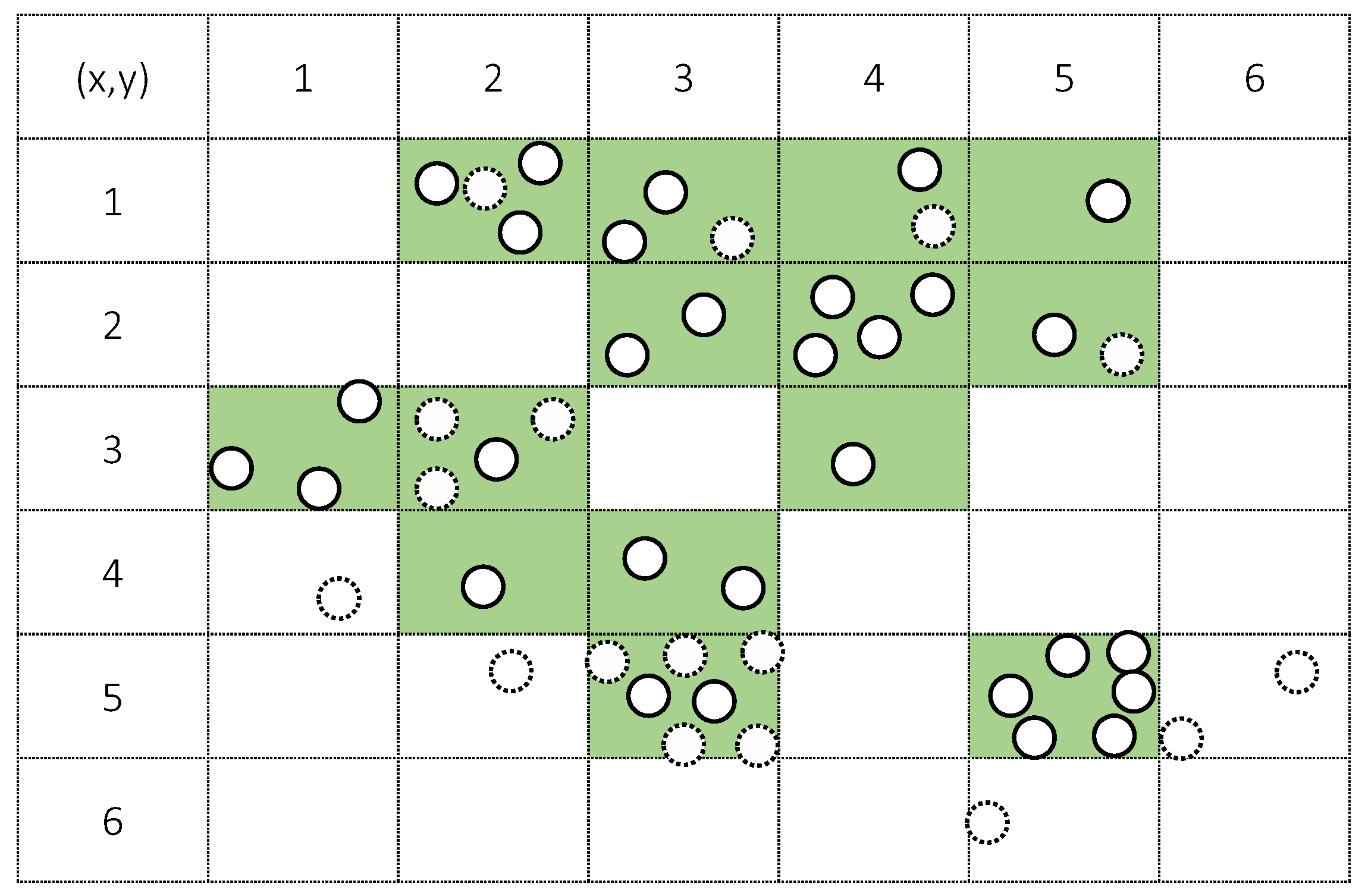
With the example of
Figure 3, the DDS selects the subset from all data on the basis of priority like
Table 1 in the case of {1/6, 1, 15} for {
rg,
m,
n}.
The DDS only considers the distribution of a target class, and thus ignores other class data in each grid. Additionally,
m data are selected from the high priority to the low priority. In the case in which the priority is the same, one grid is selected randomly.
Figure 4 shows this data selection process.
There are 2, 3, 4, and 1 target data in four grids (cylinders in the figure) in the left of
Figure 4. Because
m is equal to one, one datum is selected from all grids in the first search and the fourth grid becomes empty. Thus, in the second search, one datum is selected from the three grids. This process is run continually until
n data are selected in total.
On the basis of the DDS method, we considered the DC of data for further development. In other words, it is a method used to assign weights to the grids by measuring the consistency ratio of the target class data. This is measured by (1).
where, the division of
ntarget by
ntotal represents the ratio of the target data contained in the grid. The purpose of this study was to select the ones with high DC (
weightconsistency) to investigate the learning influence. However, we also examined the cases that selected the subset according to a descending order, called low DC (= 1 −
weightconsistency). In
Table 2, the overall process of data selection is shown using the distribution represented in
Figure 3.
Table 2 shows the conceptual examples of data selection based on the high DC and low DC simultaneously. The strategy in which data are selected is different from the DDS. This is summarized in
Figure 5.
Data selection started with the input of a set combination {
n,
rg,
m’}, namely, with the number of subset data, the grid ratio, and the number of grids selected in a single calculation, respectively. Herein,
m’ is different from
m (of DDS), which denotes the number of data selected from each grid. As shown in
Figure 5, DC selects one grid (
m’ = 1) or three grids (
m’ = 3) according to the DC weight iteratively until
n number of data are filled. The data in each grid is selected randomly, and is the same as the DDS.
Using the DC weight proposed in this study, we selected a wide range of subsets, and experimented with the data regarding their learning performance.
4. Experimental Analysis
4.1. Experimental Environmental
The experiment was conducted as follows.
Data: this method can be applied to every type of image. However, in this case we focused on CIFAR-10 only that contained real-world images with very small sizes and on difficult mage classification tasks [
19].
Training set configuration: CIFAR-10 is composed of ten classes, and each class consists of 5000 and 1000 images for training and testing, respectively. Herein, 3000, 2500, 2000, 1500, 1000, 500, 250, 200, 150, and 100 data from the original set were selected to form the training subsets, and the entire test set was used for all classification tasks. The selection of data was based on the three criteria: random selection, the high-DC weight, and the low-DC weight.
Classification model configuration: The CIFAR-10 dataset is considerably different from that obtained from MNIST and requires complex convolutional neural network architecture. Therefore, in this study, a convolution model with 14 hidden layers was configured, as shown in
Table 3. By using this model, a test accuracy of approximately 0.7846 (average value of results of five iterations—the same operation was applied to all subsequent experiments) was achieved when the classification model was trained with the entire training data.
We compared the test accuracies of the trained model with the subsets selected by three different ways.
4.2. Test Accuracy of Random Selection
First, we measured the learning performance of the subsets selected randomly. As mentioned in
Section 4.1, we prepared five sets of each subset by random selection from the entire CIFAR-10 dataset and the subsets consisted of 30,000, 25,000, 20,000, 15,000, 10,000, 5000, 2500, 2000, 1500, and 1000 data respectively. We trained the model of
Table 3 with the prepared data, and tested each model with 10,000 test set. We calculated their accuracies (correct answer rates) on average and
Figure 6 summarizes the result.
An accuracy of 0.7846 was obtained with the entire dataset (50,000 in total), and its value decreases to 0.7518, 0.7092, and to smaller values with fewer training subsets.
It is natural that learning performance improves as the number of data increases, but the degree of improvement is not directly proportional to the number of data. That is, randomly increasing the number of data or creating a model by using the entire dataset from the beginning may be costly in terms of computation time, while its performance improvement is limited. This is one of the major reasons for which we developed a data selection method that can positively influence the learning performance. There is a Selection via Proxy (SVP) method which is one of the latest research work for core data selection [
19]. The SVP compared its performance with random selection. From this aspect, we also aimed to derive superior performance compared with the case of randomly selected data.
4.3. Learning Performance according to Distribution Consistency
To investigate the effect of DC proposed in
Section 3.2, various combinations of {
rg,
mʹ,
n} were formed as follows:
rg: {0.5, 0.25, 0.2, 0.125, 0.1, 0.05, 0.04, 0.025, 0.02, 0.01, 0.008, 0.005}. These are decimal numbers that can be divided by unity without leaving a remainder. Grids with sizes of 2 × 2 are formed in the case of 0.5 and of 200 × 200 in the case of 0.005.
mʹ: {1} means that m’ is equal to one. Up to this now, we only considered how effective the distribution consistency and the grid ratio are.
n: {30,000, 25,000, 20,000, 15,000, 10,000, 5000, 2500, 2000, 1500, 1000}. This sequence is the same as the random selection described in
Section 4.2.
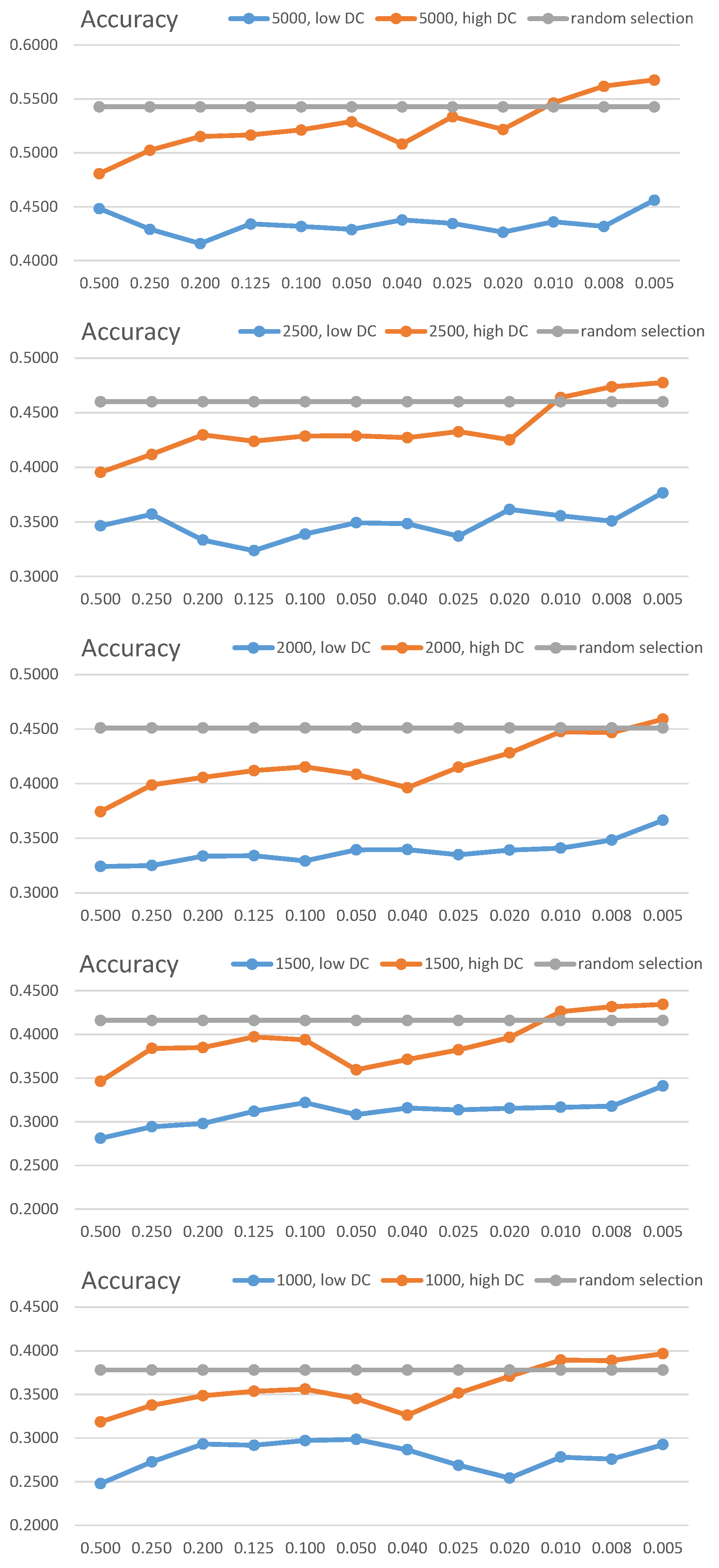
In these configurations, we trained the classification model with the data obtained from each combination, and applied the model to the test set. This process was iterated five times to calculate the average accuracy. A summary of the results is shown in
Figure 7.
In
Figure 7, the results of training and tests are shown using datasets of size
n from the top to the bottom. The orange line indicates the accuracies of high DC, the blue line is the low DC, and the gray line means the random selection. The overall test results, based on these combinations, indicate that the data selected based on the high DC positively influence the increases in the test accuracy. In addition, it can be observed that the detailed subdivision of the grids increases the performance. In the case of CIFAR-10, the complexity of the data is high, and it is thus difficult to show outcomes superior to the learning performance of randomly selected data. However, we could confirm that superior accuracy was achieved when the grid ratios of 0.008 and 0.005 were used, compared with the case of random selection.
We compared the accuracies with the random selection and the DDS.
Figure 8 shows the comparison outcomes. The DDS shows the best accuracy for a 60% selection but it is not the case in others, even when it achieved the worst performance (selection of data less than 40%). Conversely, the DC achieved stable accuracies within the entire selection range.
In summary, the implication of this study is associated with the fact that we can enhance the learning performance when we select the data based on the detailed grid ratio and the priority depending on the high DC values. We could confirm this with
Figure 7 that consistently shows the better accuracies in the combination of the detailed grids (specifically, 0.008 and 0.005) and high DC. Moreover, the high DC attained more stable data selection, as shown in
Figure 8, than that of DDS. DDS showed the best accuracies in two cases (60% and 50% data selection) but decreased drastically in lesser data selection. On the other hand, the high DC method has the stable and the best performance in general.
To identify the reason for this implication, we investigated the distribution of selected data based on high and low DCs.
Table 4 and
Table 5 show the data distributions for one class. Each distribution contains all the data (5000 orange and blue points), wherein orange points denote the selected data and blue points do not. Herein, from the difference in the DC, it can be observed that the cases associated with high DC select data from a dense area, and the cases associated with low DC select data from a sparse area. Considering that high DC exhibits superior performance, this finding is the opposite of the premise of prior research [
16] in which the data distributed in similar areas were found to have similar contributions to the learning performance. In addition, we can check that as the grid ratio decreases and becomes more refined, the area in which data are selected is expanded. These results empirically demonstrate that data selection from a wide area with a high DC can positively contribute to the learning performance.
4.4. Time-Efficiency Analsysis
Because a routine for selecting core subsets for ML is added prior to the classifier, additional time is required for computation. First, we measured the elapsed time for learning with different numbers of data, and
Figure 9 shows the result. Evidently, more time is needed when more data are available, but the performance does not improve considerably (refer to
Figure 8). This means that the time for HITL can be shortened by starting with a small amount of data to create an optimal ML model. Furthermore, the method can be utilized for various applications such as data selection for active learning, curriculum learning, and others. These points indicate why it is important to form core subsets for efficient training.
The time for data selection is added to the aforementioned classifier, and the DC method is expected to expend approximately 13.28 s, as shown in
Table 6. The selection process is performed just once before entering the stage of ML. This means that it is independent of the HITL process which requires the maximum amount of time and cost to create AI. In addition, it can be regarded that the added time is not large compared with the time taken for model training, especially in view of the fact that the method demonstrates better performance compared with random selection.
5. Conclusions
We suggested a method that selected core subsets to contribute positively to the learning performance. For this purpose, we investigated the effects on test accuracy according to the DC of training data. Specifically, we employed the InceptionV3 model to interpret complex images, and the t-SNE method to reduce to low n-dimensions, especially to two-dimensional planes for easy understanding. Furthermore, we divided the plane into grids at fixed ratios, and calculated weights with the use of high DC and low DC of each grid. As a result, we confirmed that the learning performance could be better when training data were selected in conditions in which the grid ratio was less than 0.008, and the distribution consistency was high. In addition, this selection achieved the best performance that was more stable than those of DDS and random selection.
ML is an AI development tool and it accompanies an HITL process in which humans are repeatedly involved until they reach the desired performance in the development of automatic and intelligent software. It is almost impossible to reach the targeted performance in a few trials. Instead, additional data collection, data preprocessing, model selection, and hyper-parameter tuning are needed, but these require significant amounts of time and cost. The method proposed in this study is related to the data collection in the HITL and can contribute to shortening the HITL time to derive the optimal model with a smaller amount of data. Moreover, the results of this study present the criteria for selecting training data that improve the learning performance, rather than using indiscreetly large amounts of data when additional data are needed, including active learning. In addition, the findings of this study can be utilized in the development of a strategy for the selection of training data in curriculum learning to quickly reach the global minimum point of the loss function when training is performed with the entire set of acquired data.
Based on this viewpoint, numerous additional studies ought to be conducted. We will investigate the performance change by setting the diversity of m’ values by changing various representation learning models and dimensional reduction methods, and by applying newly improved selection methods. Furthermore, we will use various benchmarking datasets. Overall, we will apply the selection methods for active and curriculum learning.
Author Contributions
Conceptualization, M.H., Y.J., and W.-K.S.; methodology, M.H., Y.J.; software, M.H.; validation, M.H., Y.J.; investigation, M.H., Y.J.; resources, W.-K.S.; data curation, M.H., Y.J.; writing original draft preparation, M.H.; writing—review and editing, M.H., Y.J.; visualization, M.H.; supervision, Y.J. and W.-K.S.; project administration, W.-K.S.; funding acquisition, W.-K.S. All authors have read and agreed to the published version of the manuscript.
Funding
This research was funded by Korea Institute of Science and Technology Information (KISTI).
Institutional Review Board Statement
Not applicable.
Informed Consent Statement
Not applicable.
Data Availability Statement
Data sharing not applicable.
Conflicts of Interest
The Authors declare no conflict of interest.
References
- Greff, K.; Srivastava, R.K.; Koutník, J.; Steunebrink, B.R.; Schmidhuber, J. LSTM: A search space odyssey. IEEE Trans. Neural Netw. Learn. Syst. 2017, 28, 2222–2232. [Google Scholar] [CrossRef] [PubMed]
- He, K.; Zhang, X.; Ren, S.; Sun, J. Deep residual learning for image recognition. In Proceedings of the IEEE Conference on Computer Vision and Pattern Recognition (CVPR), Las Vegas, NV, USA, 26 June–1 July 2016; pp. 770–778. [Google Scholar]
- Huang, Y.; Cheng, Y.; Bapna, A.; Firat, O.; Chen, M.; Chen, D.; Lee, H.; Ngiam, J.; Le, Q.; Wu, Y.; et al. GPipe: Efficient training of giant neural networks using pipeline parallelism. In Proceedings of the Vanco 33rd Conference on Neural Information Processing Systems (NeurIPS 2019), Vancouver, BC, Canada, 8–14 December 2019; pp. 103–112. [Google Scholar]
- Krizhevsky, A. Learning Multiple Layers of Features from Tiny Images. In Technical Report TR-2009; University of Toronto: Toronto, ON, Canada, 2009. [Google Scholar]
- Krizhevsky, A.; Sutskever, I.; Hinton, G.E. ImageNet classification with deep convolutional neural networks. Adv. Neural Inf. Proc. Syst. 2012, 25, 1097–1105. [Google Scholar] [CrossRef]
- Liu, X.; Shen, Y.; Duh, K.; Gao, J. Stochastic answer networks for machine reading comprehension. In Proceedings of the 56th Annual Meeting of the Association for Computational Linguistics (ACL 2018), Melbourne, Australia, 15–20 July 2018; pp. 1694–1704. [Google Scholar]
- Lu, Z.; Deb, K.; Boddeti, V. MUXConv: Information multiplexing in convolutional neural networks. In Proceedings of the IEEE/CVF Conference on Computer Vision and Pattern Recognition, Seattle, WA, USA, 13–19 June 2020; pp. 12041–12050. [Google Scholar]
- Maaten, L.V.D.; Hinton, G. Visualizing data using t-SNE. J. Mach. Learn. Res. 2008, 9, 2579–2605. [Google Scholar]
- Mikolov, T.; Sutskever, I.; Chen, K.; Corrado, G.S.; Dean, J. Distributed representations of words and phrases and their compositionality. In Proceedings of the Advances in Neural Information Processing Systems (NIPS 2013), Lake Tahoe, NV, USA, 5–10 December 2013; pp. 3111–3119. [Google Scholar]
- Pearson, K. LIII. On lines and planes of closest fit to systems of points in space. Lond. Edinb. Dublin Philos. Magaz. J. Sci. 1901, 2, 559–572. [Google Scholar] [CrossRef]
- Roh, Y.; Heo, G.; Whang, S.E. A survey on data collection for machine learning: A big data-AI integration perspective. IEEE Trans. Knowl. Data Eng. 2019. [Google Scholar] [CrossRef]
- Szegedy, C.; Liu, W.; Jia, Y.; Sermanet, P.; Reed, S.; Anguelov, S.; Erhan, D.; Vanhoucke, V.; Rabinovich, A. Going deeper with convolutions. In Proceedings of the IEEE Conference on Computer Vision and Pattern Recognition, Boston, MA, USA, 7–12 June 2015; pp. 1–9. [Google Scholar]
- Szegedy, C.; Vanhoucke, V.; Ioffe, S.; Shlens, J.; Wojna, Z. Rethinking the inception architecture for computer vision. In Proceedings of the IEEE Conference on Computer Vision and Pattern Recognition, Las Vegas, NV, USA, 26 June–1 July 2016; pp. 2818–2826. [Google Scholar]
- Tan, M.; Le, Q. EfficientNet: Rethinking model scaling for convolutional neural networks. In Proceedings of the 36th International Conference on Machine Learning, Long Beach, CA, USA, 9–15 June 2019; pp. 6105–6114. [Google Scholar]
- Tenenbaum, J.B.; De Silva, V.; Langford, J.C. A global geometric framework for nonlinear dimensionality reduction. Science 2000, 290, 2319–2323. [Google Scholar] [CrossRef] [PubMed]
- Xin, D.; Ma, L.; Liu, J.; Macke, S.; Song, S.; Parameswaran, A. HELIX: Accelerating human-in-the-loop machine learning. In Proceedings of the VLDB Endowment, Rio de Janeiro, Brazil, 3 August 2018; pp. 446–460. [Google Scholar]
- Zhang, Z.; Wu, Y.; Zhou, J.; Duan, S.; Zhao, H.; Wang, R. SG-Net: Syntax-guided machine reading comprehension. In Proceedings of the Thirty-Fourth AAAI Conference on Artificial Intelligence, New York, NY, USA, 7–12 February 2020; pp. 9636–9643. [Google Scholar]
- Hwang, M.; Jeong, Y.; Sung, W. Data distribution search to select core-set for machine learning. In Proceedings of the 9th International Conference on Smart Media & Applications (SMA 2020), Jeju, Korea, 17–19 September 2020. [Google Scholar]
- Coleman, C.; Mussmann, C.; Mirzasoleiman, B.; Bailis, P.; Liang, P.; Leskovec, J.; Zaharia, M. Selection via proxy: Efficient data selection for deep learning. In Proceedings of the International Conference on Learning Representations, Addis Ababa, Ethiopia, 30 April 2020. [Google Scholar]
| Publisher’s Note: MDPI stays neutral with regard to jurisdictional claims in published maps and institutional affiliations. |
© 2021 by the authors. Licensee MDPI, Basel, Switzerland. This article is an open access article distributed under the terms and conditions of the Creative Commons Attribution (CC BY) license (http://creativecommons.org/licenses/by/4.0/).


