1. Introduction
A production line is typically a set of equipment or machines established in a factory where components are assembled sequentially to make a finished product [
1]. Nowadays, manufacturers use different kinds of machines for production, and over time, these machines and the associated equipment may deteriorate, and sometimes even the entire production line may fail [
2]. Breakdowns seriously impact the performance and cost of production lines and often lead to a dramatic reduction of availability because of the costly maintenance period [
3].
For avoiding these failure cases, the maintenance of resources is often planned in advance [
4]. However, the maintenance cost of some industries can increase by up to 70% of the total cost [
5]. As such, the reduction of maintenance costs is considered a crucial and substantial advantage to the manufacturer in a highly competitive manufacturing sector, such as, for example, the semiconductor industry. In many industrial sectors such as automotive manufacturing, maintenance management is an explicit strategic issue to take necessary actions on time [
6,
7]. Fixing the production line after the breakdown can be more costly than conducting preventive maintenance ahead of the breakdown [
8,
9]. Also, the revision of the production plan can cause variability in service and product quality [
1].
One of the approaches to reducing maintenance costs is known as preventive maintenance. Preventive maintenance can be considered as a kind of proactive approach, which systematically inspects and maintain the equipment to avoid breakdowns. There exist several factors that can complicate the maintenance operation of production lines, such as system configurations, cost of maintenance resources, degradation profiles of machines, maintenance schedule, and recent status of machines [
10].
From a machine learning perspective, there are several challenges of preventive maintenance in production lines. First, it is indeed difficult to acquire machine malfunction data and label the failure case in practice in the datasets. Second, there exists a huge amount of process data (i.e., big data) generated in production lines, and processing of this big data requires a special infrastructure, expert knowledge, and custom smart software. Last, many companies do not share this type of data publicly due to data privacy, and as such, researchers in this field are unable to validate new models with more datasets. To this end, there is a need for further research to come up with effective measures and new models in order to implement predictive maintenance effectively in production lines.
Remaining useful life (RUL) is a key metric and critical to predicting the failure of a machine in the production line. The challenge of RUL prediction is that RUL is not mostly labeled in the training dataset, and therefore, supervised learning algorithms of machine learning cannot be applied in this case. A health index needs to be correctly defined and interpolated to map the relationship between features and the RUL. After this interpolation step, a machine learning-based model can be used to predict the health index by learning the interpolated data accurately. The machine learning-based approach is expected to handle the adverse impacts of noise in the dataset and possible sensor problems (i.e., sensor drift) that might arise during the operation of the production line.
The main objective of our study is to minimize the adverse effects of breakdowns and build a novel machine learning-based RUL prediction model. We propose and validate a new machine learning-based model in predicting the failure of equipment (i.e., RUL prediction) in production lines and analyze the applicability of machine learning algorithms in predicting the failure of equipment in product lines. Specifically, we focus on jet engines and use the run-to-failure data of similar jet engines to predict the failures of jet engines. This data includes several measurements including temperatures, pressures, rotating speeds of jet engines. During our experiments, different machine learning algorithms, pre-processing and feature selection techniques, and parameter optimization approaches are investigated to build a novel model to predict the risk of production line failure.
The concept of RUL is used to evaluate the risk of production line breakdown. For the case study, the NASA dataset on turbo engines has been used in this study [
11]. The proposed model developed in this case study can also be applied to the other production lines. The case study demonstrates the effectiveness of our prediction model to predict the RUL within the scope of predictive maintenance.
The contributions of this study are two-fold, which are listed as follows:
We developed a novel RUL prediction approach that utilizes the principal component analysis (PCA) feature selection algorithm, grid search parameter optimization algorithm, and multi-layer perceptron (MLP) machine learning algorithm.
Since the RUL was not provided in training datasets, a polynomial function was fitted to HIs, and the interception between the polynomial and cycle axis was calculated as the failure point.
The following sections of this article are organized as follows:
Section 2 explains the background and related work.
Section 3 presents the data analysis.
Section 4 describes the methodology, and
Section 5 explains the experimental results.
Section 6 presents the discussion and threats to validity.
Section 7 presents conclusions and future work.
2. Background and Related Work
Four categories of maintenance policies have been suggested in the literature [
12]: run-to-failure (R2F), preventive maintenance (PM), condition-based maintenance (CBM), and predictive maintenance (PdM). R2F is executed after the failure, and as such, this is the simplest approach and the costliest one, among others. PM is performed periodically based on a schedule. CBM checks several conditions, and if one of them indicates that there is a degradation of the equipment, CBM is directly executed. PdM (a.k.a., statistical-based maintenance) applies predictive analytics and tools to determine the required actions. As in the case of CBM, PdM also performs the maintenance only when it is necessary. Several authors [
12,
13] emphasize that CBM and PdM are actually addressing the same maintenance policy, and as such, they do not distinguish between them.
Many modeling approaches have been used in literature for maintenance policy analysis and reliability engineering [
2]. Some of these approaches are Markov chains [
14,
15], Petri nets [
16], fault tree analysis [
17], and analytic hierarchy process [
18]. Also, quantitative methods have been proposed using heuristic methods [
19], simulation techniques [
20], and analytical methods [
2].
Seiti et al. [
21] used a multi-criteria decision-making (MCDM) method based on fuzzy probability and D number to evaluate the breakdown risk of a production line. The MCDM provides a risk rank of a machine breakdown from high to low, which is useful for decision making. However, the model highly relies on expert knowledge, and the result of the prediction is subjective to the risk grade given by the expert.
Bayesian network (BN) is an effective algorithm to handle complex systems like production lines, and the possibility of applying BN in production line lifetime prediction is investigated by Wang et al. [
22]. A simulation model is also an option for lifetime prediction, and a study showed that the stochastic simulation model achieved high accuracy in predicting the lifetime of a rectifier system [
11]. The drawback of the simulation model is that it requires expert knowledge to build.
Among approaches used for PdM, machine learning-based ones are considered to be the most suitable approaches because they can handle high-dimensional problems that consist of hundreds or thousands of variables such as voltages, flows, and currents [
23]. There exist two main categories of machine learning-based techniques for PdM. The first one is supervised approaches where the failure information exists in the dataset. The second one is unsupervised approaches, where there is only process information, and no failure-related information exists [
23].
Machine learning methods have been increasingly applied in different areas to perform various tasks. Fault diagnosis is the most common application area of machine learning, which determines whether to send equipment to fix (or to be replaced). This kind of task mainly uses binary classification or multi-category classification algorithms to predict failures or malfunctions. Luo and Wang [
24] applied random forest to identify the malfunction of robot arms by learning patterns from the torque sensors. However, there is a lack of models to predict the remaining lifetime of a machine because there are not enough indicators to measure the health status of a machine [
25]. Also, the health status is largely affected by the operating environment, and some failure is caused by accident rather than deterioration.
As a result of the wide adoption of machine learning techniques in many application fields, recently, researchers focused on the use of machine learning techniques for predicting the machine lifetime. RUL is mostly used as a risk indicator for preventive maintenance service. It indicates how long a machine can operate as usual before the breakdown. RUL modeling requires a run-to-failure dataset from the operation of machines, which is difficult to acquire.
A set of turbo engine run-to-failure datasets is provided by NASA [
26], and the data is used in many research papers to predict the RUL. Ramasso and Saxena [
27] published a survey on prognostic methods used for the NASA turbo engine datasets and divided the prognostic approaches into three categories. The first category is the use of functional mappings between the set of inputs and RUL. For the first category, they reported that the dominant underlying machine learning algorithm is artificial neural networks (ANNs). The second category of techniques is the functional mapping between the health index and RUL. The third category is similarity-based matching techniques. Benchmarking of prognostic methods has been conducted on the NASA turbo engine dataset, and it was shown that most of the studies use a health index to map between input features and the RUL [
27].
Research on RUL prediction can be divided into the following categories [
28]: knowledge-based models (KBM), physical models (PM), data-driven models (DDM), and deep learning (DL). In knowledge-based models, experts define the rule sets and evaluate the condition of the equipment based on previous failures and sometimes they result in contradictions [
29]. Physical models model the complete equipment, however, it is expensive and not always achievable. Early data-driven models used statistical and stochastic approaches such as Markov models, proportional hazard modelling, and Bayesian techniques with Kalman filters [
30]. There is an assumption of stochastic models. Identical components are considered to be statistically identical and random variables are independent. However, this assumption is not true for some datasets that include random starting conditions. In general, statistical approaches form a hypothesis before building the model and work on several assumptions. Each statistical approach comes with a different assumption. However, in machine learning, algorithms are run on data directly. Also, machine learning-based approaches often provide better performance than statistical approaches in terms of accuracy though more computational power is required in recent years. To avoid the limitations of statistical and stochastic models and achieve higher performance, we aimed to focus on machine learning approaches instead of developing models using statistical methods.
Ahmadzadeh and Lundberg [
31] published a review article in 2013 and categorized the RUL prediction studies into the following four categories:
Physics-based: Physical model, cumulative damage, hazard rate, proportional hazard rate, nonlinear dynamics
Experimental-based
Data-driven: Neural network (NN), support vector machine, Bayesian network, hidden (Markov, semi-Markov)
Hybrid: Statistical model, Fourier transform with NN, statistical model with NN, fuzzy logic with NN, wavelet transform analysis with a statistical model, dynamic wavelet with NN.
They also provided the advantages and disadvantages of these approaches. Physics-based approaches are computationally expensive, too stochastic to model the fault, and need the evaluation of assumptions. Experimental approaches are costly and required to verify the theoretical models. Data-driven approaches use nonlinear relationships and perform pattern recognition. Hybrid methods combine two methodologies such as statistical methods and neural networks. They reported that the best model is selected based on the availability of the data [
31].
Okoh et al. [
32] classified studies into the following RUL prediction methodology types in 2014: Model-based, analytical-based, knowledge-based, and hybrid. Also, they presented the following prediction technique types: Statistics, experience, computational intelligence (CI), physics-of-failure, and fusion. Artificial neural networks are represented under the CI category. They also presented in a table that while statistics-based approaches are unable to process large datasets, CI techniques are able to handle large datasets.
Hu et al. [
33] categorized RUL prediction techniques into the following three categories: Physics-based approaches, data-driven techniques (probabilistic, artificial intelligence methods, and stochastic), and hybrid approaches that combine the physics-based and data-driven techniques. They proposed the state space model (SSM) for RUL prediction.
Si et al. [
34] reviewed statistical data-driven approaches and categorized the condition monitoring (CM) data into direct CM data and indirect CM data. Under the direct CM data, the following approaches were presented: Regression-based, Wiener process, gamma process, and Markovian-based. Under the indirect CM data, the following techniques were provided: Stochastic filtering-based, covariate-based hazard, and hidden Markov model & hidden semi-Markov model-based. They discussed several challenges related to the RUL prediction. For example, they stated that a new RUL prediction model is required in the case of very limited observed failure data or no observed failure data because statistical models cannot be used in these two cases.
Djeziri et al. [
35] categorized the RUL estimation approaches into the following categories:
As we see in these six review articles [
28,
31,
32,
33,
34,
35], different researchers categorized RUL prediction studies into different categories, however, main techniques, namely machine learning, statistical models, physics-based techniques, hybrid approaches, and knowledge/expert-based approaches often appear in these taxonomies.
Recently, deep learning-based RUL prediction models have been proposed. Li et al. [
36] developed a multi-scale deep convolutional neural network (MS-DCNN) and used the min-max normalization with the MS-DCNN algorithm for RUL prediction. They compared the performance of their model with other state-of-the-art models and showed that the new model provides promising results on the NASA C-MAPSS dataset.
Hou et al. [
37] developed a deep supervised learning approach using similarity to improve the prediction performance. Since the health indicator (HI) construction techniques depend on manual labeling or expert opinion, Hou et al. [
37] also developed an unsupervised learning approach-based on restricted Boltzmann machine (RBM) to construct the HI. They showed that their performance provides superior performance compared to the other traditional approaches. Cheng et al. [
38] proposed a transferable convolutional neural network (TCNN) to learn domain invariant features for bearing RUL prediction. They showed that their model avoids the influence of kernel selection and present a better performance for RUL prediction. Wang et al. [
39] proposed a recurrent convolutional neural network (RCNN) for RUL prediction and demonstrated its effectiveness based on two case studies. They showed that the proposed model can predict the RUL prediction of rolling element bearings and milling cutters effectively. Their model provides a probabilistic result for RUL prediction and simplifies decision making. Chen et al. [
40] developed a recurrent neural network (RNN) model using an encoder-decoder structure with an attention mechanism for RUL prediction of rolling bearings. They showed that their model can work with little prior knowledge and provides better performance than the other models. Wu et al. [
41] proposed a deep long short-term memory (DLSTM) network that uses the grid search strategy for RUL prediction. They demonstrated that this model provides satisfactory performance for the RUL prediction of turbofan engines. Li et al. [
42] applied the generative adversarial network (GAN) algorithm to compute the distribution of the healthy state data and proposed a health indicator. Promising results were achieved on two rotating machinery datasets. Su et al. [
43] integrated the variational autoencoder (VAE) algorithm with a time-window-based sequence neural network (twSNN) for RUL prediction and demonstrated the effectiveness of their model on a dataset of aircraft turbine engines.
While deep learning-based models can provide better performance for RUL prediction, there are several limitations of using this type of algorithms. For instance, they need a lot of data, hyperparameter tuning is required, and there is a high computational cost. To avoid these limitations, in this study we aimed to develop a novel machine learning model that is still accurate but does not consist of these limitations.
In our study, MLP that is a special ANN topology, along with other machine learning methods (i.e., grid search parameter optimization, normalization, and feature selection), are combined with the interpolation technique, and a novel machine learning-based RUL prediction model is built. The effectiveness of this new model is investigated on NASA turbo engine datasets.
3. Data Analysis
There are four turbofan datasets running on different conditions, as shown in
Table 1. For instance, the dataset FD001 has 100 turbo engine units running under one condition with only a high-pressure cylinder (HPC) fault. In the training dataset, the turbo running from a certain point to failure while in the testing dataset, the records stop at a middle point. The task is to predict the RUL of the turbofan in the testing dataset. In other words, an algorithm needs to predict when the turbo will break, and the required maintenance is needed. In
Table 2, the data structure of the training dataset is presented, and in
Table 3, the data structure of the RUL dataset is shown. Settings data and sensory data are all anonymous data.
The data distribution of each dataset is different, and this difference is associated with several operating conditions and fault modes, as shown in
Table 1. The setting variables and sensor variables can be constant, discrete, and continuous. The same variable can have different data distribution forms in different datasets. For instance, the variable setting1 is a continuous variable with normal distribution in the dataset FD001_train, as shown in
Figure 1, while it is a discrete variable distributed on six values in the dataset FD002_train, as shown in
Figure 2. Similarly, the variable sensor1 changes from a constant value in the FD003_train, as shown in
Figure 3 to a discrete distribution in the dataset FD004_train, as shown in
Figure 4. In general, features of dataset FD001 and FD003 are mostly continuously distributed while the features of FD002 and FD004 are discretely distributed.
The value range of each feature varies significantly within the same dataset. In the dataset FD001_train, setting1 ranges from −0.087 to 0.087, while sensor7 ranges from 549 to 556, as shown in
Figure 1. Additionally, the range of the same variable changes dramatically in different datasets. The range of setting 1 in FDD02 & FD004_train is (0–40), as shown in
Figure 2 and
Figure 4 while the range in FD001 and FD003 is (−0.087–0.087) as shown in
Figure 1 and
Figure 3. This can be explained by the fact that FD001 has only one operation condition, while FD002 has six different conditions.
According to our observations, the setting variables’ distributions reflect the operation condition of each dataset. Datasets FD001 and FD003 operate under the same condition and have similar setting variable value distribution. FD002 and FD004 operate under six different conditions, and their variable value distributions are similar. The correlations between features are also strong.
Figure 5 presents the correlation plot of variables (sensor2, sensor3, and sensor4) of the FD001dataset.,
Figure 6 shows that some sensors are highly correlated.
4. Methodology
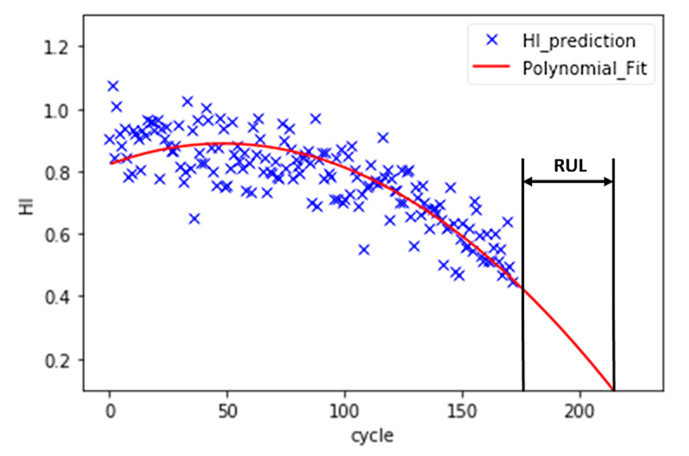
Instead of direct measurements of RUL, usually, indirect measures are adopted. For this reason, the concept of the health index (HI) is often used to estimate the RUL [
44]. Instead of directly predicting the RUL, a machine learning model is trained to predict the HI of a turbo engine in each cycle. Since the RUL is not provided in training datasets, the use of supervised learning approaches to predict the RUL label is not possible. Then, a polynomial function is fitted to HIs, and the interception between the polynomial and cycle axis is the failure point. In
Figure 7, this approach and the calculation of RUL is represented.
In the training datasets, each turbo machine runs from good health conditions to failure one. Thus, this research assumes the HI of initial cycles is maximum and the HI of last cycles is minimum. Therefore, we can assume that N initial cycles that have HI = 1, and N last cycles that have HI = 0. Then, the rest of the data points label can be estimated by interpolation. After the interpolation, all points are labeled and supervised learning can be applied.
Figure 8 represents the flowchart of our interpolation and machine learning-based prediction model. First, a model is trained with partially labeled data. Then, the trained model is used to interpolate the rest of the unlabeled training points with HIs. After the interpolation, the entire HI labeled dataset is used as a feedback mechanism for the model to re-train the model.
4.1. Data Pre-Processing
Some features are constant in the dataset, and thus, their variance is zero. All zero variance variables are removed before the training stage because they do not contain useful information for machine learning. Since the value range is substantially different in different variables, it can be difficult to find the optimal point for the cost function. It also tends to take a long time to reach the optimum, which uses extra computational power. Therefore, the training and testing datasets need to be normalized. There are two widely used methods for normalization, which are Z-scores (Equation (1)) and min-max-scale (Equation (2)). Both methods are applied, and the one with the best evaluation result is selected.
The correlation heatmap shown in
Figure 6 indicates that half of the features in the dataset are highly correlated to each other. For avoiding the negative effect of the covariance, principle components analysis (PCA) is applied for features in the dataset. The number of PCA components equals the number of features to catch all the variance in the original data.
4.2. Model Selection
Two different approaches have been applied during the learning process. The first model learns from the part of the labeled dataset and conducts the interpolation for the rest of the data points. The second model learns from the entire dataset, and it uses the final model to predict the HI. For the first model, several algorithms were applied, and the linear regression (LR) achieved the best interpolation results. The results of other algorithms do not show a regular degradation trend, and as such, it is difficult to fit with a polynomial curve. Therefore, a linear regression model is selected to be the first model.
According to our literature search in electronic databases, multi-layer perceptron neural network (MLP), random forest (RF) [
45], and support vector regression (SVR) algorithms are the three most used algorithms for the PdM category. Therefore, MLP, RF, SVR, and LR are applied as the second model to perform the re-training process of the entire dataset.
The grid search cross-validation method is applied to find the best hyperparameters of RF and SVR. The best hyperparameters have the lowest HI MSE. For the RF, parameters are selected as follows: estimator = 100 and depth of tree = 6. For the SVR, the radial basis function kernel is chosen, and gamma is assigned to 0.1. For the MLP model, units and cycles are excluded from the inputs, and
Table 4 shows the parameters used in this study.
4.3. Interpolation and Model Training
There are three stages in the interpolation and re-train process, which are partial dataset training, interpolation, and full dataset training, as shown in
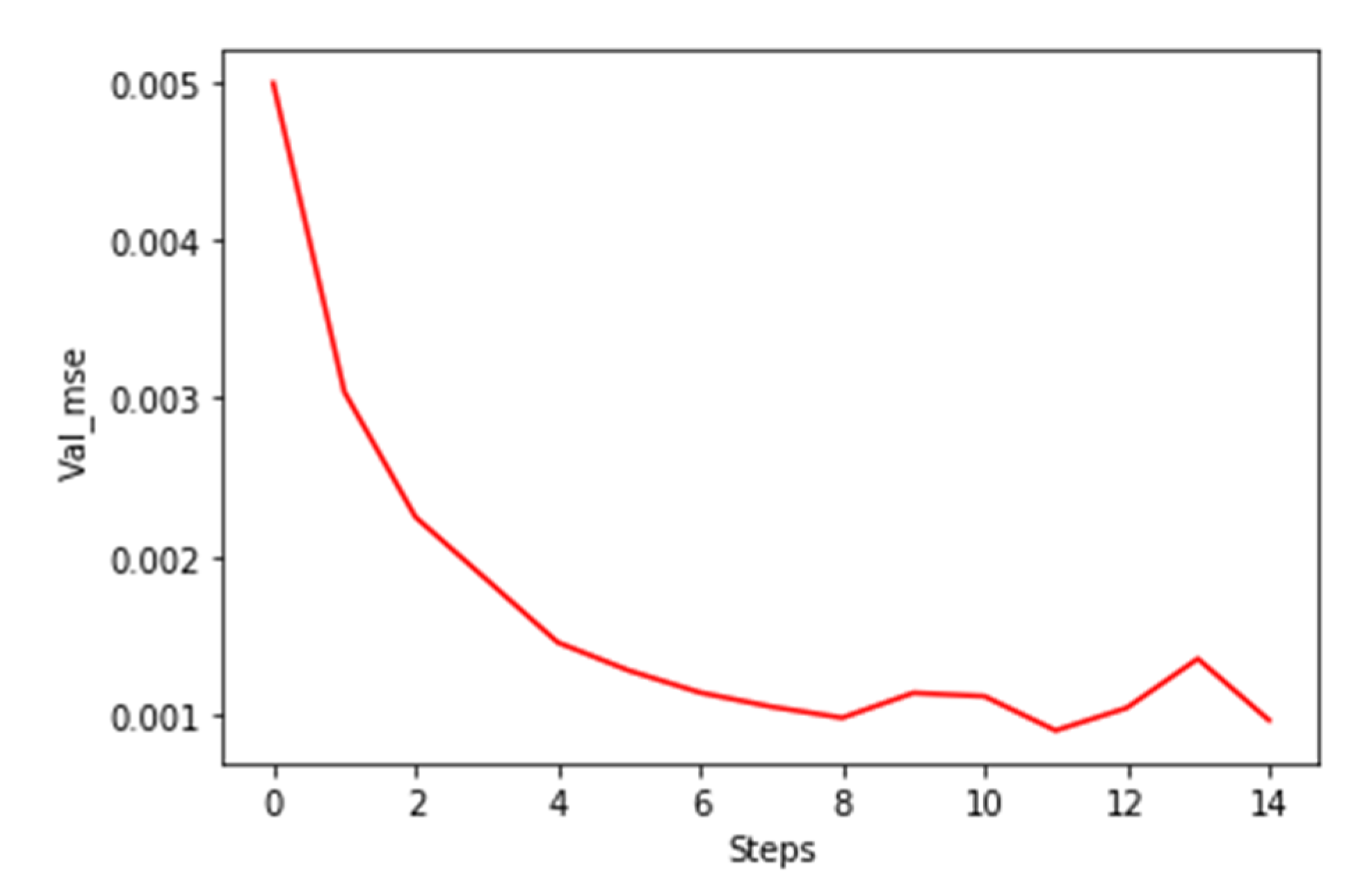
Figure 8. After the labeling process, a part of the dataset is labeled with the HI index, which can be used for supervised learning. The trained model then predicts the rest of the unlabeled data points so that the whole dataset is labeled with HI. Last, the model is re-trained with the entire labeled dataset to improve the mean squared error (MSE). 5-fold cross-validation is used to prevent overfitting in both the first and second stages. The training process stops earlier if the validation MSE stops decreasing in the next five steps, as shown in
Figure 9.
Figure 10. demonstrates the interpolation process of HI with partially labeled data points.
Figure 11 shows that a selected model learns from the entire dataset after the interpolation and predicts a similar HI pattern for each turbo unit.
4.4. Evaluation
Because the purpose of the machine learning model is to predict the RUL instead of the HI, the MSE of the training cannot be used to evaluate the performance of the model. A model may have very low training MSE, but it may have a high deviation in the RUL prediction. In other words, the tuning of hyperparameters, such as the size of N points, the number of PCA components, and model parameters, cannot rely on the training MSE. According to
Figure 7, the estimation of RUL is based on a polynomial curve fit. Therefore, a second-order polynomial (Equation (3)) is fitted to the HI. The coefficient must be a negative number to ensure that the curve is decreasing.
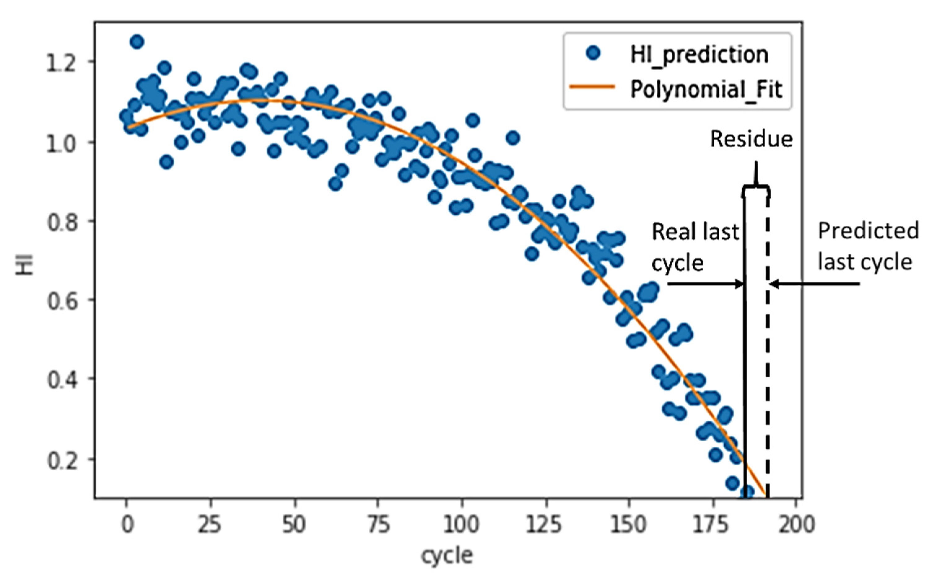
In the training dataset, the turbo engines run from healthy conditions to failure one. Therefore, the RUL at the last cycle of the training data point should be zero. The residue between the real last cycle and the predicted last cycle can be calculated, as shown in
Figure 12. The RUL MSE can then be calculated based on Equation (4). The n is equal to the number of turbo units in the dataset. T
r and T
p stand for the real last cycle and the predicted last cycle, respectively.
The model is optimized against the MSERUL by tuning hyperparameters. The model setting with the lowest MSERUL is used for validation. After training, the model needs to be validated with the testing dataset. The testing data is processed with the steps, as in the case of training data. The testing data should have the same variables as the training data, and it is normalized with the training data mean and variance if Z-scores are performed. The testing data is transferred to PCA components with the training data eigenvector matrix.
Then, the processed testing data is fed to the model to predict HI for each cycle. A second-order polynomial is fitted to the HIs with the minimum MSE. The interception between the curve and the cycle axis is the prediction of the end cycle. RUL can be calculated to subtract the last cycle of the test data from the end cycle. The MSERUL_Val can be calculated based on Equation (5). The n equals the number of turbo units in the dataset. RULr and RULp stand for the real RUL of the test data and the predicted RUL, respectively.


