
Realworld 3D Object Recognition Using a 3D Extension of the HOG Descriptor and a Depth Camera


Abstract
1. Introduction
2. Related Works
3. Methodology
3.1. Training Dataset and Data Preprocessing
- No preprocessing. The object descriptor is computed directly for each object from the training dataset.
- Subset of training objects. We selected a subset of synthetic objects from the training dataset in order to train the recognition data flow. We evaluated all the training dataset objects at , and voxel grid resolutions in order to discard those not having enough resolution. In order to determine the objects with a too low resolution, we manually evaluated each object one-by-one. The main criteria for the selection were that the object shows qualitatively distinctive features from the class it belongs to. Consequently, the evaluation contained all the objects at different voxel grid resolutions.
- Dataset augmentation. We perform a dataset augmentation by rotating each synthetic object from the training dataset along the Z axis. Hence, we generate multiple views of the same object as in Figure 2. We assume therefore, that the objects are always aligned on the X and Y axes. Otherwise, additional rotations on the X and Y axes are required.
- Frontal projection. Due to the lack of a complete 3D object shape captured by a depth camera, synthetic objects are preprocessed to compute the frontal projection according to the camera position described in Figure 3.
- Pose alignment. Each synthetic object from the training dataset is aligned using the PCA-STD method described in Vilar et al. [30] before computing the object descriptor in order to achieve rotational invariance.
3.2. Preparation of the Real Dataset
- Point cloud conversion. The depth map image captured by the camera (Figure 4) is converted to a cloud of non-structured points in 3D space. The conversion is performed using the Application Programming Interface (API) software functions provided by the camera manufacturer.
- Ground plane removal. As a first object segmentation step, the point cloud points belonging to the GP are segmented and removed using the M-estimator sample-consensus (MSAC) algorithm [31]. In addition, the estimated GP points are used to align the remaining point cloud data with respect to the GP. This alignment is performed first by computing the principal component analysis (PCA) of the estimated GP points and later by performing an affine transformation of the remaining point cloud data in order to rotate it according with the measured angles (, ) (1) of the GP. Angle measurements are performed considering that the principal components on the Z axis () are equivalent to the normal vector () of the GP, Figure 6.
- Clustering. Point cloud data above the GP are segmented into clusters based on the Euclidean distance. Minimum Euclidean distance parameter is chosen according to the experimental results.
- Pose alignment. In the same way as described for the training dataset, the segmented objects are preprocessed to normalize their pose using the PCA-STD method described in [32] in order to achieve rotational invariance.
- Voxelization. Point cloud data from the segmented cluster are then converted into a voxel-based representation. This conversion is performed first by normalizing the data size according with the voxel resolution grid, and later by approximating each point form the point cloud to the nearest voxel integer value.
3.3. Object Descriptor and Dimensionality Feature Reduction
3.4. SVM Classifier
4. Results and Analysis
4.1. Experimental Flow
4.2. Acquisition of Real World Data
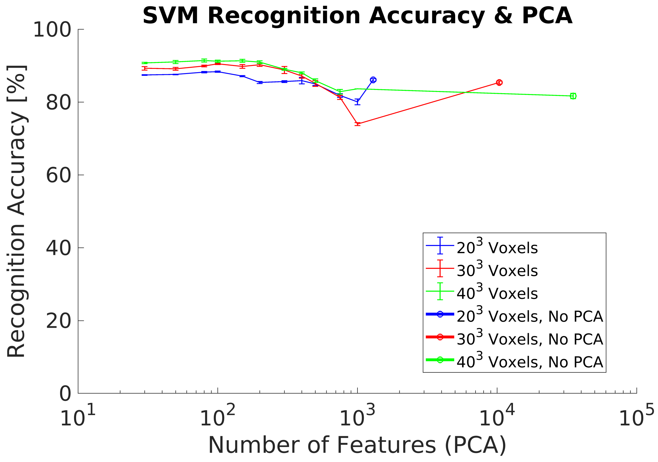
4.3. Experiment 1
4.4. Experiment 2
4.5. Experiment 3
4.6. Experiment 4
4.7. Experiment 5
4.8. Experiment 6
4.9. Experiment 7
5. Discussion
5.1. Synthetic Dataset
5.2. Real Dataset
5.3. Rotational Invariance Data Preprocessing
5.4. Frontal Projection Data Preprocessing
5.5. Subset of Synthetic Training Objects
- Glossy and no-reflective surfaces. Monitors have some areas where the structured IR light pattern is not reflected back to the camera. This error depends on the relative angle between the monitor and the camera. Thus, at certain angles, the camera can not capture the object and therefore compute any depth. As a result, it appears as a blank area in the depth computation, causing a complete distortion of the original object shape. In addition, the same effect occurs on glossy surface areas where the IR light pattern of the camera is reflected back in multiple directions.This camera drawback is specially relevant for robotic applications where it is required to detect and track surrounding objects or humans. Light absorbent materials (e.g., dark clothes) and light reflective materials can distort the depth measurement and thus limit their application scope when camera uses active illumination [30].
- Segmentation errors. Object segmentation relies on the GP’s flatness and the MSAC algorithm to estimate the GP points. Noise and depth computation errors can lead to an incomplete removal of the GP from the point cloud data. As a consequence, objects in the scene are not segmented correctly causing a distorsion of the original object shapes.
- Depth artifacts. Sharp and narrow edges in the camera image lead to shadow errors in the 3D point cloud generation and thus distort completely the object shape measurement.
5.6. Response Time
6. Conclusions
Author Contributions
Funding
Data Availability Statement
Conflicts of Interest
References
- Carvalho, L.E.; von Wangenheim, A. 3D object recognition and classification: A systematic literature review. Pattern Anal. Appl. 2019, 22, 1243–1292. [Google Scholar] [CrossRef]
- Papazov, C.; Haddadin, S.; Parusel, S.; Krieger, K.; Burschka, D. Rigid 3D geometry matching for grasping of known objects in cluttered scenes. Int. J. Robot. Res. 2012, 31, 538–553. [Google Scholar] [CrossRef]
- Izadi, S.; Kim, D.; Hilliges, O.; Molyneaux, D.; Newcombe, R.; Kohli, P.; Shotton, J.; Hodges, S.; Freeman, D.; Davison, A.; et al. KinectFusion: Real-time 3D Reconstruction and Interaction Using a Moving Depth Camera. In Proceedings of the 24th Annual ACM Symposium on User Interface Software and Technology, Santa Barbara, CA, USA, 16–19 October 2011; pp. 559–568. [Google Scholar] [CrossRef]
- Aleman, J.; Monjardin Hernandez, H.S.; Orozco-Rosas, U.; Picos, K. Autonomous navigation for a holonomic drive robot in an unknown environment using a depth camera. In Optics and Photonics for Information Processing XIV; International Society for Optics and Photonics: Bellingham, WA, USA, 2020; p. 1. [Google Scholar] [CrossRef]
- Zhi, S.; Liu, Y.; Li, X.; Guo, Y. Toward real-time 3D object recognition: A lightweight volumetric CNN framework using multitask learning. Comput. Graph. (Pergamon) 2018, 71, 199–207. [Google Scholar] [CrossRef]
- Domenech, J.F.; Escalona, F.; Gomez-Donoso, F.; Cazorla, M. A Voxelized Fractal Descriptor for 3D Object Recognition. IEEE Access 2020, 8, 161958–161968. [Google Scholar] [CrossRef]
- Wu, Z.; Song, S. 3D ShapeNets: A Deep Representation for Volumetric Shapes. In Proceedings of the Conference on Computer Vision and Pattern Recognition (CVPR), Boston, MA, USA, 7–12 June 2015; pp. 1912–1920. [Google Scholar]
- Vilar, C.; Krug, S.; Thornberg, B. Processing chain for 3D histogram of gradients based real-time object recognition. Int. J. Adv. Robot. Syst. 2020, 13. [Google Scholar] [CrossRef]
- He, Y.; Chen, S.; Yu, H.; Yang, T. A cylindrical shape descriptor for registration of unstructured point clouds from real-time 3D sensors. J. Real Time Image Process. 2020, 1–9. [Google Scholar] [CrossRef]
- Qi, C.R.; Su, H.; Mo, K.; Guibas, L.J. PointNet: Deep learning on point sets for 3D classification and segmentation. In Proceedings of the Conference on Computer Vision and Pattern Recognition (CVPR), Long Beach, CA, USA, 19–25 June 2017; pp. 77–85. [Google Scholar]
- Maturana, D.; Scherer, S. VoxNet: A 3D Convolutional Neural Network for Real-Time Object Recognition. In Proceedings of the International Conference on Intelligent Robots and Systems (IROS), Hamburg, Germany, 28 September–2 October 2015; pp. 922–928. [Google Scholar]
- Simon, M.; Amende, K.; Kraus, A.; Honer, J.; Samann, T.; Kaulbersch, H.; Milz, S.; Gross, H.M. Complexer-YOLO: Real-time 3D object detection and tracking on semantic point clouds. In Proceedings of the Computer Society Conference on Computer Vision and Pattern Recognition Workshops (CVPRW), Long Beach, CA, USA, 18–20 June 2019; pp. 1190–1199. [Google Scholar] [CrossRef]
- Yavartanoo, M.; Kim, E.Y.; Lee, K.M. SPNet: Deep 3D Object Classification and Retrieval Using Stereographic Projection. Lect. Notes Comput. Sci. 2019, 11365, 691–706. [Google Scholar]
- Bayramoglu, N.; Alatan, A.A. Shape index SIFT: Range image recognition using local features. In Proceedings of the International Conference on Pattern Recognition (ICPR), Istanbul, Turkey, 23–26 August 2010; pp. 352–355. [Google Scholar] [CrossRef]
- Tang, K.; Member, S.; Song, P.; Chen, X. 3D Object Recognition in Cluttered Scenes With Robust Shape Description and Correspondence Selection. IEEE Access 2017, 5, 1833–1845. [Google Scholar] [CrossRef]
- Salti, S.; Tombari, F.; Stefano, L.D. SHOT: Unique signatures of histograms for surface and texture description q. Comput. Vis. Image Underst. 2014, 125, 251–264. [Google Scholar] [CrossRef]
- Yang, J.; Xiao, Y.; Cao, Z. Aligning 2.5D Scene Fragments With Distinctive Local Geometric Features. IEEE Trans. Circuits Syst. Video Technol. 2019, 29, 714–729. [Google Scholar] [CrossRef]
- Tao, W.; Hua, X.; Yu, K.; Chen, X.; Zhao, B. A Pipeline for 3-D Object Recognition Based on Local Shape Description in Cluttered Scenes. IEEE Trans. Geosci. Remote. Sens. 2020, 1–16. [Google Scholar] [CrossRef]
- Do Monte Lima, J.P.S.; Teichrieb, V. An efficient global point cloud descriptor for object recognition and pose estimation. In Proceedings of the 29th Conference on Graphics, Patterns and Images (SIBGRAPI), Sao Paulo, Brazil, 4–7 October 2016; pp. 56–63. [Google Scholar] [CrossRef]
- Aldoma, A.; Tombari, F.; Di Stefano, L.; Vincze, M. A global hypotheses verification method for 3D object recognition. In Proceedings of the European Conference on Computer Vision (ECCV), Florence, Italy, 7–13 October 2012; pp. 511–524. [Google Scholar]
- Li, D.; Wang, H.; Liu, N.; Wang, X.; Xu, J. 3D Object Recognition and Pose Estimation from Point Cloud Using Stably Observed Point Pair Feature. IEEE Access 2020, 8. [Google Scholar] [CrossRef]
- Johnson, A.E.; Hebert, M. Using Spin Images for Efficient Object Recognition in Cluttered 3D Scenes. IEEE Trans. Pattern Anal. Mach. Intell. 1999, 21, 433–449. [Google Scholar] [CrossRef]
- Rusu, R.B.; Bradski, G.; Thibaux, R.; Hsu, J. Fast 3D recognition and pose using the viewpoint feature histogram. In Proceedings of the IEEE/RSJ 2010 International Conference on Intelligent Robots and Systems (IROS), Taipei, Taiwan, 18–22 October 2010; pp. 2155–2162. [Google Scholar] [CrossRef]
- Rusu, R.B.; Blodow, N.; Beetz, M. Fast Point Feature Histograms (FPFH) for 3D registration. In Proceedings of the International Conference on Robotics and Automation (ICRA), Xi’an, China, 30 May–5 June 2009; pp. 3212–3217. [Google Scholar] [CrossRef]
- Wohlkinger, W.; Vincze, M. Ensemble of shape functions for 3D object classification. In Proceedings of the International Conference on Robotics and Biomimetics (ROBIO), Karon Beach, Thailand, 7–11 December 2011; pp. 2987–2992. [Google Scholar]
- Dalal, N.; Triggs, B. Histograms of Oriented Gradients for Human Detection. In Proceedings of the 2005 IEEE Computer Society Conference on Computer Vision and Pattern Recognition (CVPR’05), San Diego, CA, USA, 20–25 June 2005; pp. 886–893. [Google Scholar]
- Dupre, R.; Argyriou, V. 3D Voxel HOG and Risk Estimation. In Proceedings of the International Conference on Digital Signal Processing (DSP), Singapore, 21–24 July 2015; pp. 482–486. [Google Scholar]
- Scherer, M.; Walter, M.; Schreck, T. Histograms of oriented gradients for 3d object retrieval. In Proceedings of the 18th International Conference in Central Europe on Computer Graphics, Visualization and Computer Vision (WSCG), Plzen, Czech Republic, 1–4 February 2010; pp. 41–48. [Google Scholar]
- Buch, N.; Orwell, J.; Velastin, S.A. 3D extended histogram of oriented gradients (3DHOG) for classification of road users in urban scenes. In Proceedings of the British Machine Vision Conference (BMVC), London, UK, 7–10 September 2009. [Google Scholar] [CrossRef][Green Version]
- Vilar, C.; Thörnberg, B.; Krug, S. Evaluation of Embedded Camera Systems for Autonomous Wheelchairs. In Proceedings of the 5th International Conference on Vehicle Technology and Intelligent Transport Systems (VEHITS), Crete, Greece, 3–5 May 2019; pp. 76–85. [Google Scholar] [CrossRef]
- Torr, P.H.S.; Zisserman, A. MLESAC: A new robust estimator with application to estimating image geometry. Comput. Vis. Image Underst. 2000, 78, 138–156. [Google Scholar] [CrossRef]
- Vilar, C.; Krug, S.; Thornberg, B. Rotational Invariant Object Recognition for Robotic Vision. In Proceedings of the 3rd International Conference on Automation, Control and Robots (ICACR), Shanghai, China, 1–3 August 2019; pp. 1–6. [Google Scholar]


| Dataset | Bottle | Bowl | Chair | Cup | Keyboard | Lamp | Laptop | Monitor | Plant | Stool | |
|---|---|---|---|---|---|---|---|---|---|---|---|
| Training | 335 | 64 | 889 | 79 | 145 | 124 | 149 | 465 | 240 | 90 | 2580 |
| Augmentation. | |||||||||||
| Training | 2680 | 512 | 7112 | 632 | 1160 | 992 | 1192 | 3720 | 1920 | 720 | 20,640 |
| Sub.&Augmentation. | |||||||||||
| Training | 816 | 448 | 1096 | 288 | 560 | 472 | 536 | 712 | 648 | 528 | 6104 |
| Synthetic | |||||||||||
| Test | 99 | 19 | 99 | 19 | 19 | 19 | 19 | 99 | 99 | 19 | 510 |
| Camera | |||||||||||
| Test | 64 | 48 | 64 | 64 | 48 | 48 | 48 | 48 | 48 | 48 | 528 |
| Voxel Grid | |||
|---|---|---|---|
| 1 | 8 | 27 | |
| 8 | 8 | 8 | |
| 1296 | 10,368 | 34,992 |
| Parameter | Value |
|---|---|
| 18 | |
| 9 | |
| 6 | |
| 2 | |
| 2 |
| Parameter | SVM Classifier |
|---|---|
| Type | Multiclass |
| Method | Error correcting codes (ECOC) |
| Kernel function | Radial basis function |
| Optimization | Iterative single data (ISDA) |
| Data division | Holdout partition 15% |
| Exp. | Training Dataset | Test Dataset | Acc. Results | ||
|---|---|---|---|---|---|
| 1 | Synthetic | No preprocessing | Synthetic | No preprocessing | 91.5% |
| 2 | Synthetic | PCA-STD alignment | Synthetic | PCA-STD align. | 90% |
| 3 | Synthetic | No preprocessing | Real | No preprocessing | 65% |
| 4 | Synthetic | PCA-STD alignment | Real | PCA-STD align. | 21% |
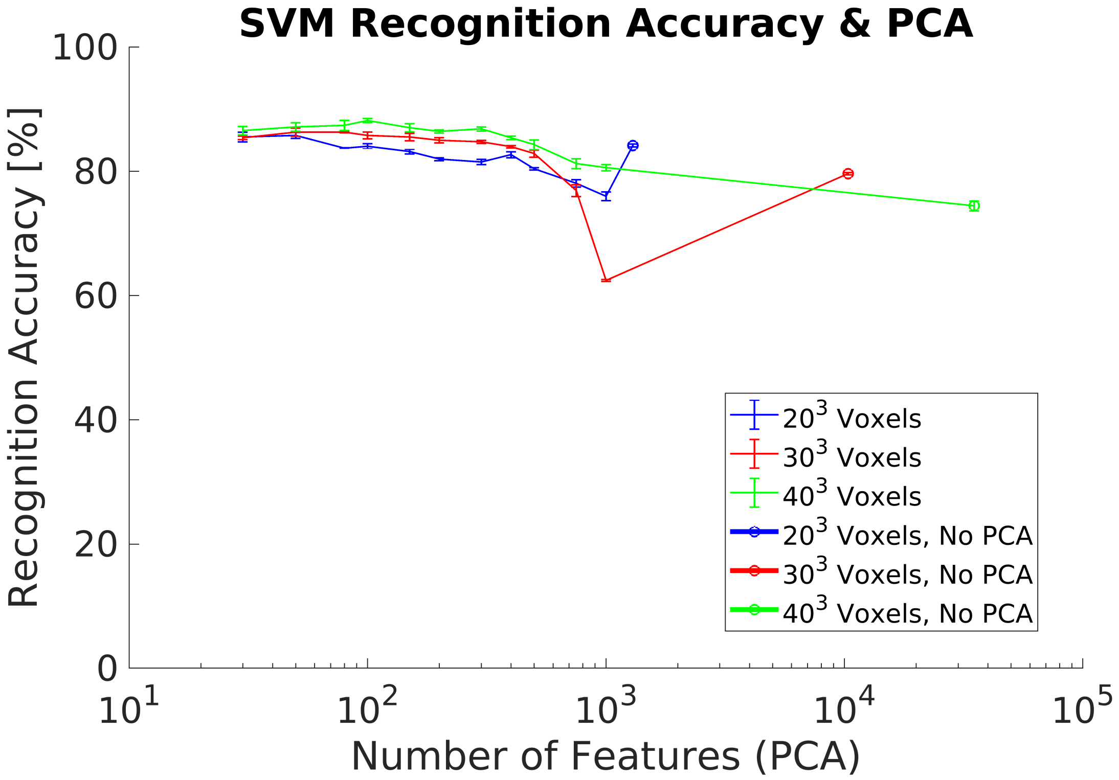
| 5 | Synthetic | Dataset augm. | Real | No preprocessing | 75.7% |
| 6 | Synthetic | Dataset augm. + Frontal view | Real | No preprocessing | 73.7% |
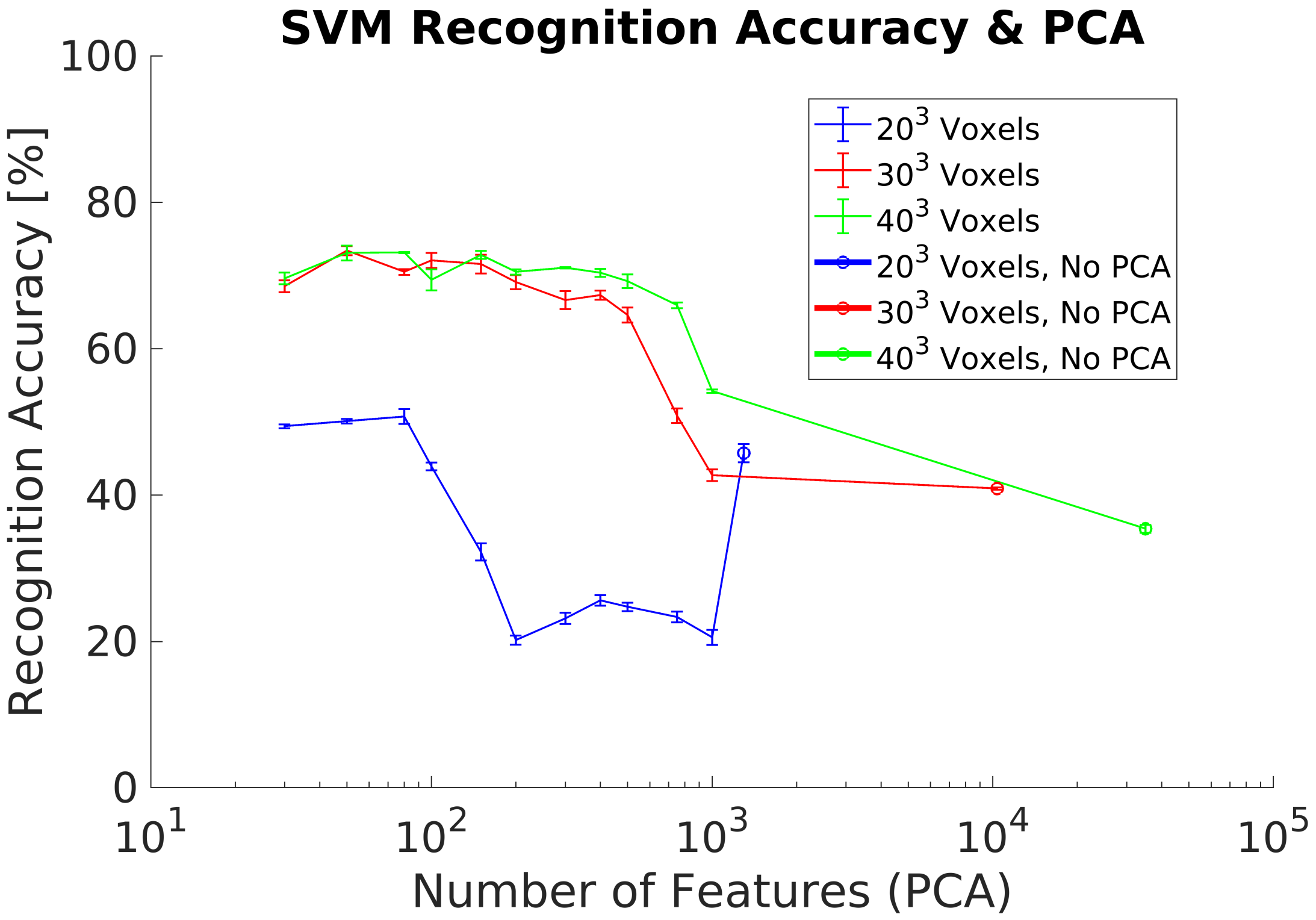
| 7 | Synthetic | Dataset augm. + Frontal view + Subset | Real | No preprocessing | 81.5% |
| Technology | Active IR Stereo |
|---|---|
| Sensor Technology | Global shutter, 3 × 3 m |
| Depth Field-of-View | 86 × 57 |
| Depth Resolution | up to 1280 × 720 pixels |
| RGB Resolution | 1920 × 1080 pixels |
| Depth Frame Rate | up to 90 fps |
| RGB Frame Rate | 30 fps |
| Min Depth range | 0.1 m |
| Max Depth range | 10 m |
| Dimensions | 90, 25, 25 mm |
| Estimated Class | 1 | 0.98 | 0 | 0 | 0.04 | 0.02 | 0 | 0.02 | 0.02 | 0 | 0 |
| 2 | 0 | 0.98 | 0.03 | 0 | 0 | 0 | 0 | 0 | 0 | 0 | |
| 3 | 0 | 0 | 0.86 | 0 | 0 | 0 | 0 | 0 | 0.02 | 0.2 | |
| 4 | 0.01 | 0 | 0 | 0.86 | 0 | 0.14 | 0 | 0 | 0 | 0 | |
| 5 | 0 | 0 | 0 | 0 | 0.95 | 0 | 0 | 0 | 0 | 0.02 | |
| 6 | 0 | 0 | 0.01 | 0.04 | 0 | 0.85 | 0.04 | 0.12 | 0 | 0.04 | |
| 7 | 0 | 0.02 | 0 | 0 | 0.03 | 0 | 0.73 | 0.18 | 0 | 0.04 | |
| 8 | 0 | 0 | 0.09 | 0.05 | 0 | 0 | 0.15 | 0.60 | 0 | 0.40 | |
| 9 | 0.01 | 0 | 0.01 | 0.01 | 0 | 0.01 | 0.06 | 0.06 | 0.85 | 0 | |
| 10 | 0 | 0 | 0 | 0 | 0 | 0 | 0 | 0 | 0.13 | 0.30 | |
| 1 | 2 | 3 | 4 | 5 | 6 | 7 | 8 | 9 | 10 | ||
| Input Class | |||||||||||
| Test Dataset | (%) | (ms) | (ms) | (ms) | (ms) | |||
|---|---|---|---|---|---|---|---|---|
| Synthetic | 34,992 | 100 | 90 | 9 | 11.5 | 6 | 20.5 | 38 |
| Real | 34,992 | 300 | 81.5 | — | 12 | 4 | 180 | 196 |
| Approach | Method | Training Dataset | Test Dataset | 3D Sensor | Accuracy | GPU | |
|---|---|---|---|---|---|---|---|
| 3DHOG | Global | ModelNet40 | Real Custom | Stereo | 81.5% | No | 196 ms |
| 3DHOG [32] | Global | ModelNet10 | ModelNet10 | – | 84.91% | No | 21.6 ms |
| VoxNet [11] | CNN | ModelNet10 | ModelNet10 | – | 92% | Yes | 3 ms |
| PointNet [10] | CNN | ModelNet10 | ModelNet10 | – | 77.6% | Yes | 24.6 ms |
| 3DYolo [12] | CNN | KITTY | KITTY | Lidar | 75.7% | Yes | 100 ms |
| SPNet [13] | CNN | ModelNet10 | ModelNet10 | – | 97.25% | Yes | – |
| VFH [23] | Global | Real Custom | Real Custom | Stereo | 98.52% | – | – |
| SI [22,23] | Global | Real Custom | Real Custom | Stereo | 75.3% | – | – |
| VFD [6] | Global | ModelNet10 | ModelNet10 | – | 92.84% | No | – |
| RCS [17] | Local | UWA | UWA | – | 97.3% | No | 10–40 s |
| TriLCI [18] | Local | BL | BL | – | 97.2% | No | 10 s |
Publisher’s Note: MDPI stays neutral with regard to jurisdictional claims in published maps and institutional affiliations. |
© 2021 by the authors. Licensee MDPI, Basel, Switzerland. This article is an open access article distributed under the terms and conditions of the Creative Commons Attribution (CC BY) license (http://creativecommons.org/licenses/by/4.0/).
Share and Cite
Vilar, C.; Krug, S.; O’Nils, M. Realworld 3D Object Recognition Using a 3D Extension of the HOG Descriptor and a Depth Camera. Sensors 2021, 21, 910. https://doi.org/10.3390/s21030910
Vilar C, Krug S, O’Nils M. Realworld 3D Object Recognition Using a 3D Extension of the HOG Descriptor and a Depth Camera. Sensors. 2021; 21(3):910. https://doi.org/10.3390/s21030910
Chicago/Turabian StyleVilar, Cristian, Silvia Krug, and Mattias O’Nils. 2021. "Realworld 3D Object Recognition Using a 3D Extension of the HOG Descriptor and a Depth Camera" Sensors 21, no. 3: 910. https://doi.org/10.3390/s21030910
APA StyleVilar, C., Krug, S., & O’Nils, M. (2021). Realworld 3D Object Recognition Using a 3D Extension of the HOG Descriptor and a Depth Camera. Sensors, 21(3), 910. https://doi.org/10.3390/s21030910