Semantic Segmentation Leveraging Simultaneous Depth Estimation


Abstract
1. Introduction
- We propose a method to guide the RGB image semantic segmentation using depth information extracted from a depth estimation network.
- We propose a novel fusion strategy based on the multi-branch network architecture, which allows encoders with different structures to combine with each other and improves the segmentation performance.
- We train several networks using our proposed method on the ADE20k [22] dataset without any extra data source. Experiments show that our method can improve the segmentation performance compared with the baseline model.
2. Related Work
2.1. Semantic Segmentation Networks
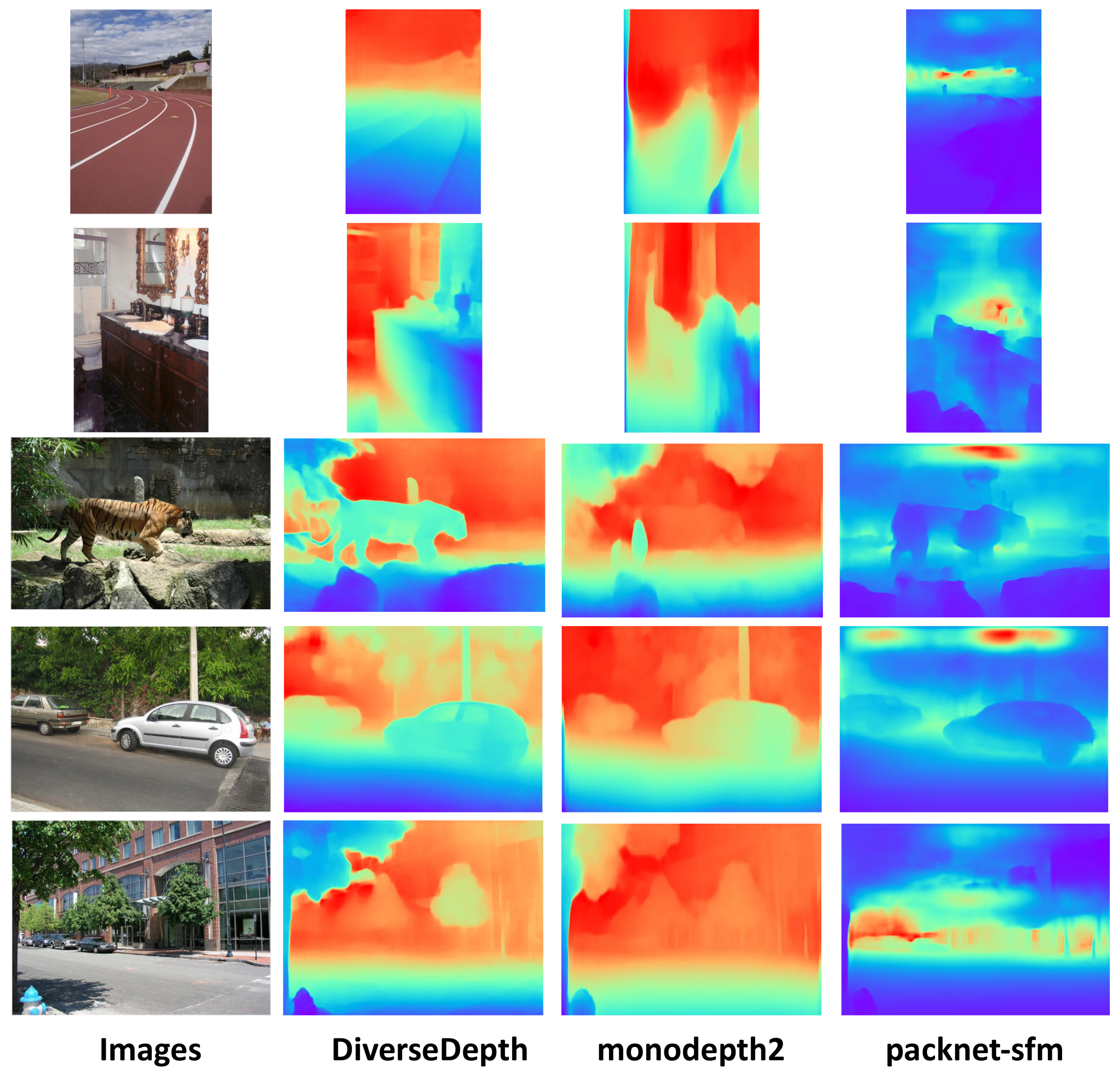
2.2. Depth from a Single Image
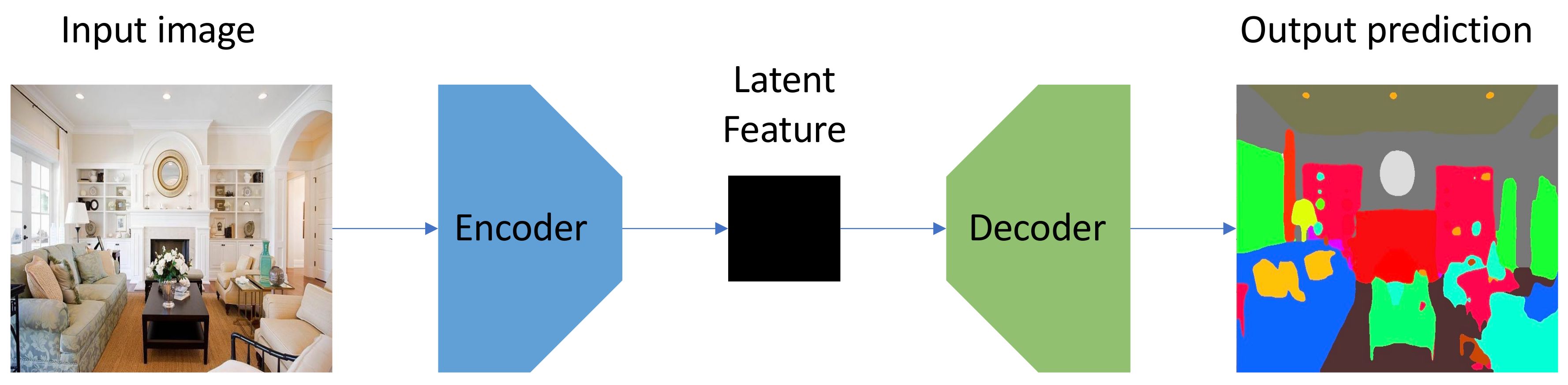
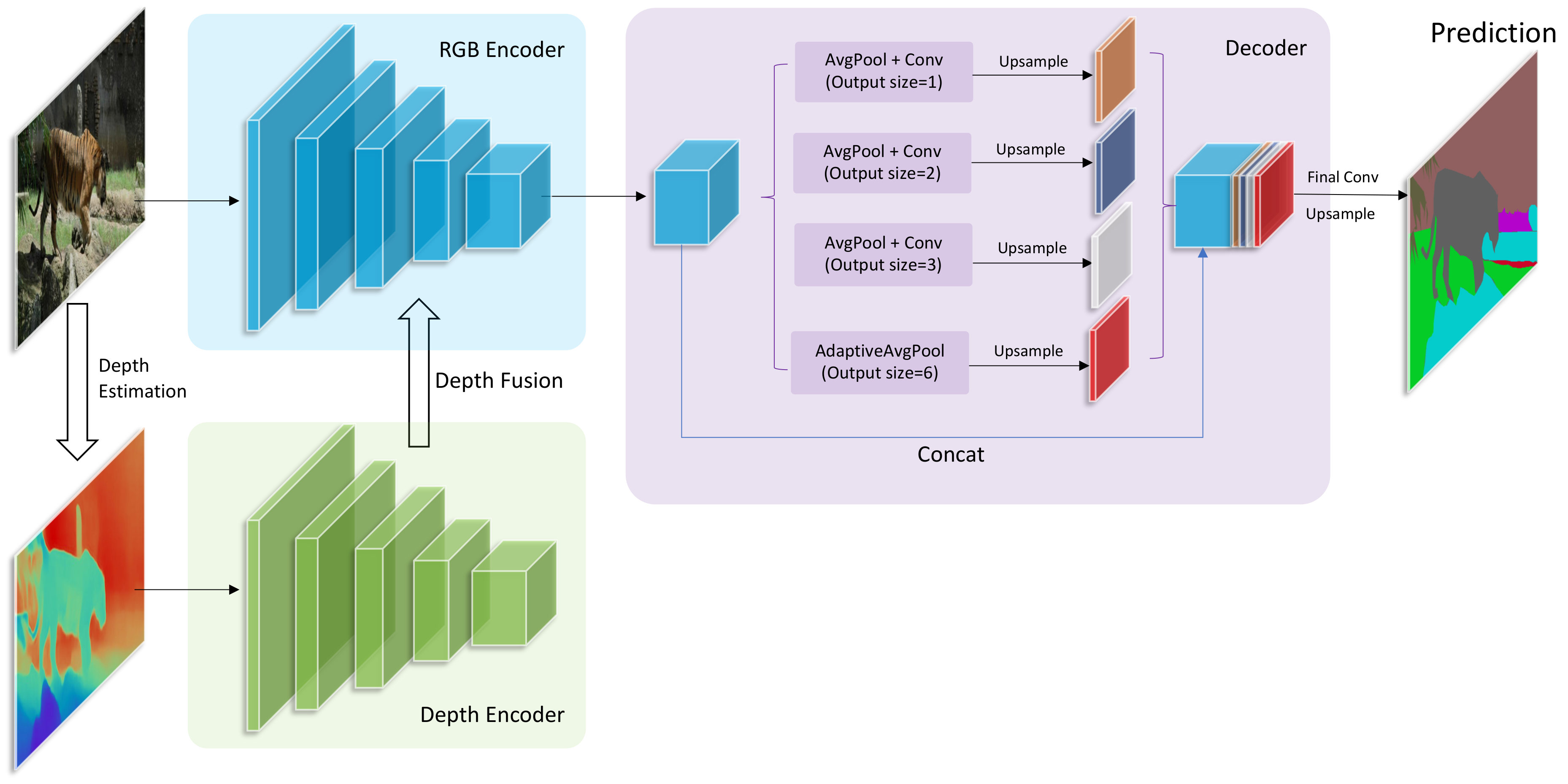
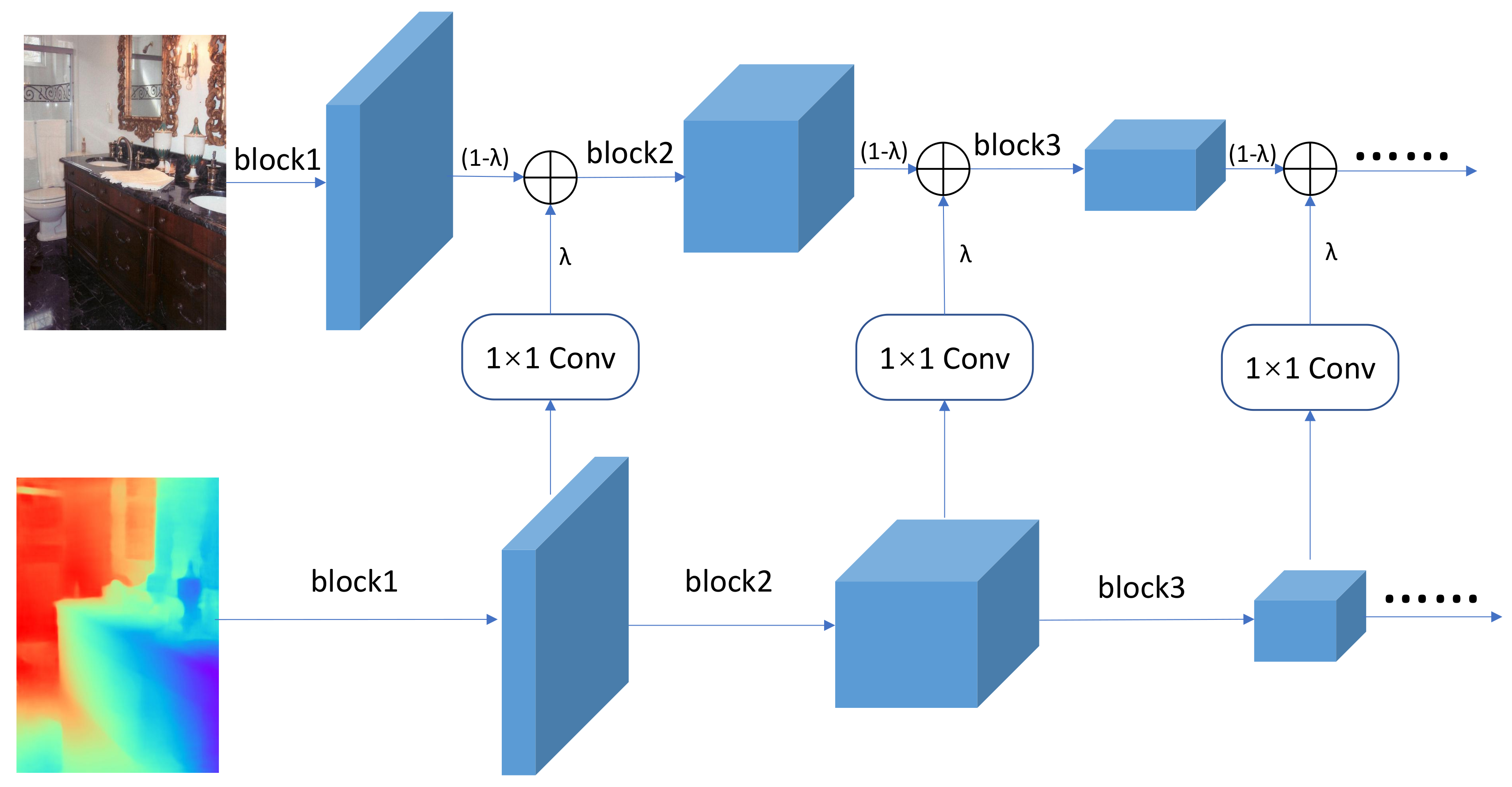
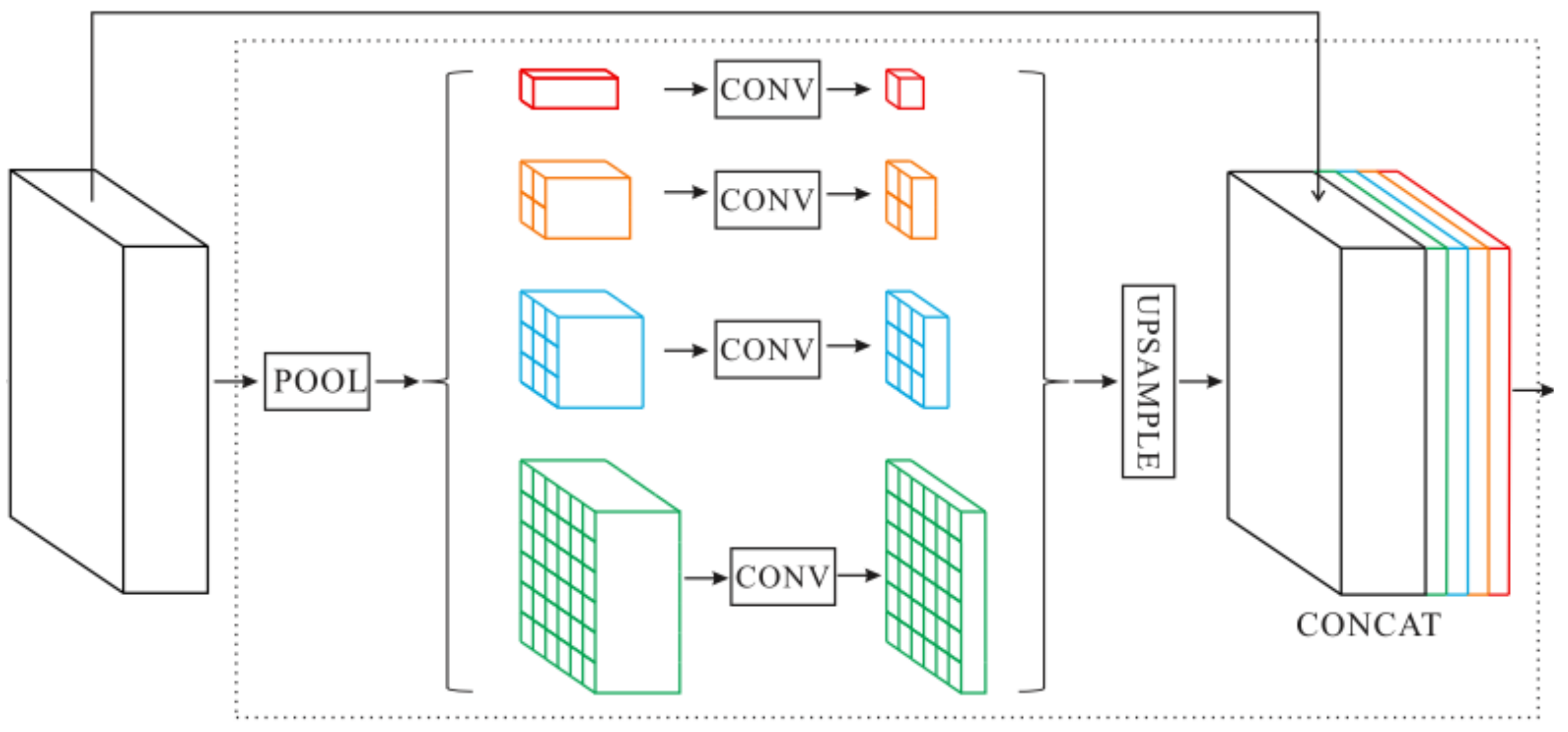
3. Method
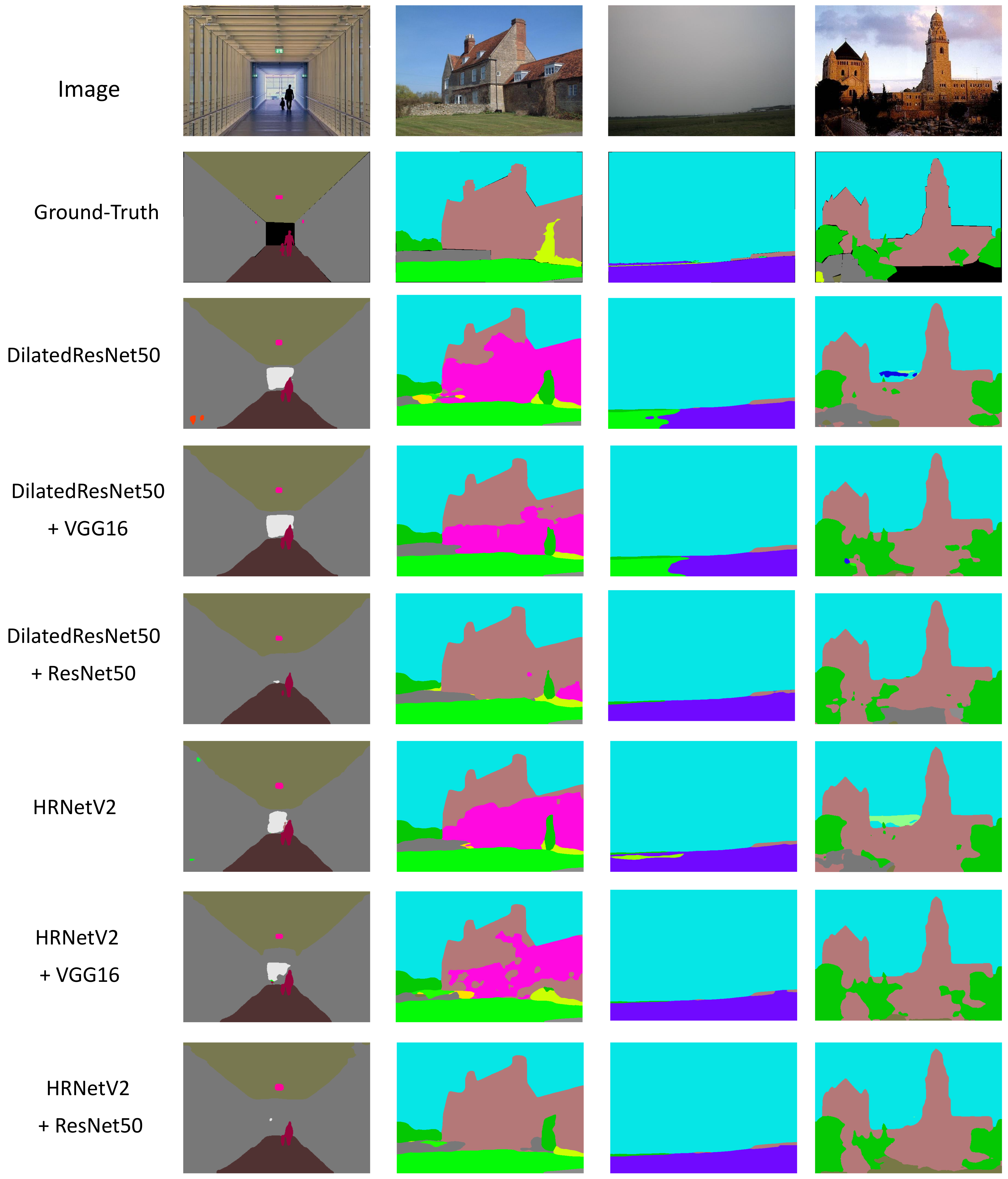
3.1. Segmentation Network Structure
3.1.1. RGB Encoder and Depth Encoder
3.1.2. Fusion Strategies
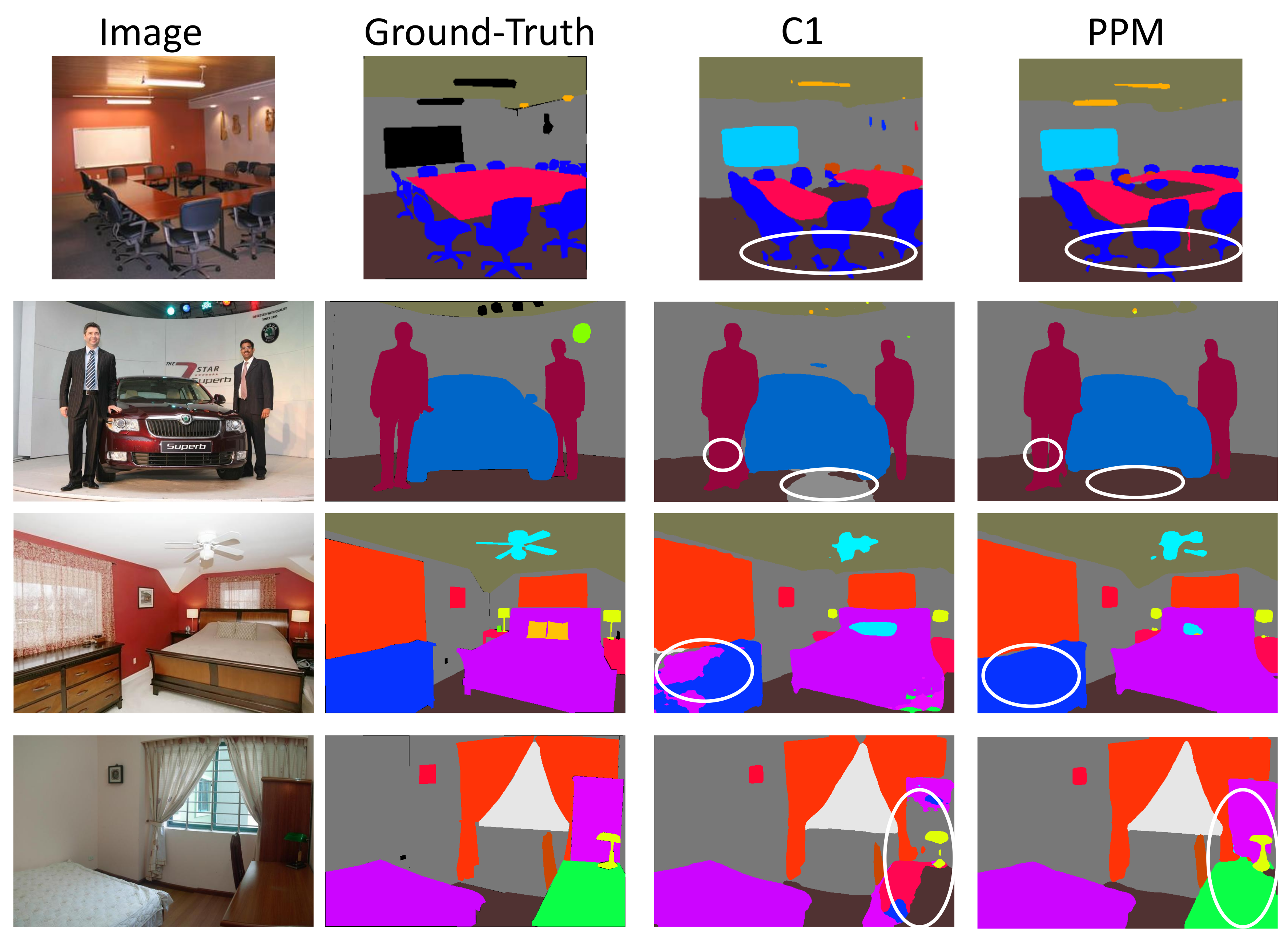
3.1.3. Decoder
3.2. Depth Estimation Network
4. Experiment
4.1. Dataset and Experiment Configuration
4.1.1. Dataset
4.1.2. Experiment Configuration
4.2. Experimental Results
4.3. Ablation Study
4.3.1. Fusion Approach
4.3.2. Fused Ratio Coefficient
4.3.3. Decoder
4.3.4. Multi-Scale Testing
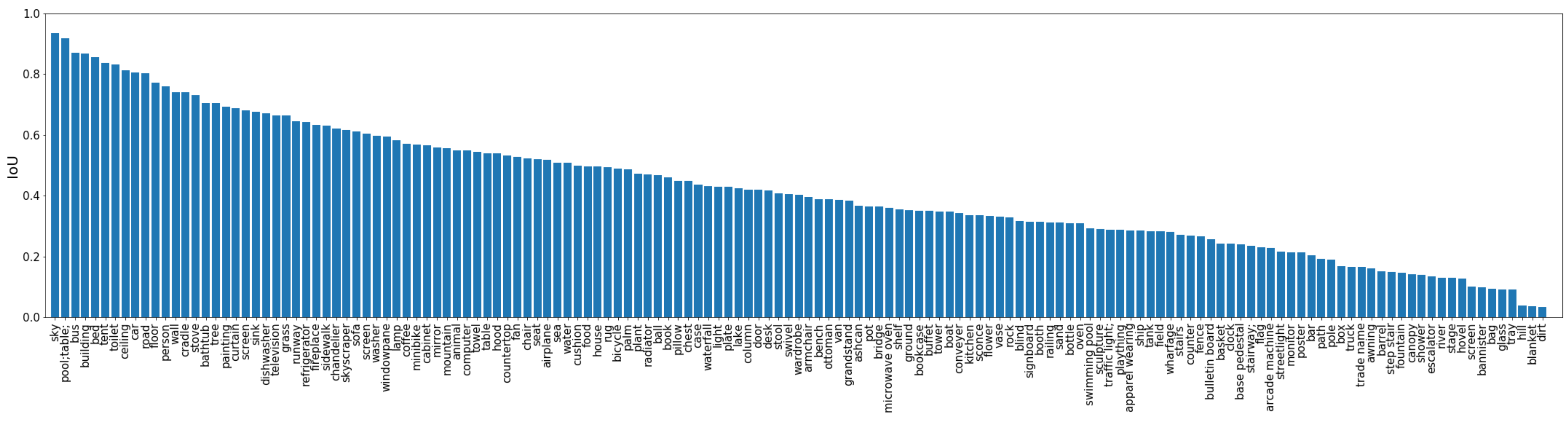
4.3.5. Performance on Each Category of Objects
5. Conclusions
Author Contributions
Funding
Institutional Review Board Statement
Informed Consent Statement
Data Availability Statement
Acknowledgments
Conflicts of Interest
References
- Zhang, H.; Geiger, A.; Urtasun, R. Understanding high-level semantics by modeling traffic patterns. In Proceedings of the IEEE International Conference on Computer Vision, Sydney, Australia, 1–8 December 2013; pp. 3056–3063. [Google Scholar]
- Ros, G.; Sellart, L.; Materzynska, J.; Vazquez, D.; Lopez, A.M. The synthia dataset: A large collection of synthetic images for semantic segmentation of urban scenes. In Proceedings of the 2016 IEEE Conference on Computer Vision and Pattern Recognition, Las Vegas, NV, USA, 27–30 June 2016; pp. 3234–3243. [Google Scholar]
- Bojarski, M.; Del Testa, D.; Dworakowski, D.; Firner, B.; Flepp, B.; Goyal, P.; Jackel, L.D.; Monfort, M.; Muller, U.; Zhang, J.; et al. End to end learning for self-driving cars. arXiv 2016, arXiv:1604.07316. [Google Scholar]
- Valada, A.; Oliveira, G.L.; Brox, T.; Burgard, W. Deep multispectral semantic scene understanding of forested environments using multimodal fusion. In Proceedings of the International Symposium on Experimental Robotics, Tokyo, Japan, 3–6 October 2016; pp. 465–477. [Google Scholar]
- Vineet, V.; Miksik, O.; Lidegaard, M.; Nießner, M.; Golodetz, S.; Prisacariu, V.A.; Kähler, O.; Murray, D.W.; Izadi, S.; Pérez, P.; et al. Incremental dense semantic stereo fusion for large-scale semantic scene reconstruction. In Proceedings of the 2015 IEEE International Conference on Robotics and Automation (ICRA), Seattle, WA, USA, 26–30 May 2015; pp. 75–82. [Google Scholar]
- Çiçek, Ö.; Abdulkadir, A.; Lienkamp, S.S.; Brox, T.; Ronneberger, O. 3D U-Net: Learning dense volumetric segmentation from sparse annotation. In Proceedings of the International Conference on Medical Image Computing and Computer-Assisted Intervention, Athens, Greece, 17–21 October 2016; pp. 424–432. [Google Scholar]
- Miksik, O.; Vineet, V.; Lidegaard, M.; Prasaath, R.; Nießner, M.; Golodetz, S.; Hicks, S.L.; Pérez, P.; Izadi, S.; Torr, P.H. The semantic paintbrush: Interactive 3d mapping and recognition in large outdoor spaces. In Proceedings of the 33rd Annual ACM Conference on Human Factors in Computing Systems, Seoul, Korea, 18–23 April 2015; pp. 3317–3326. [Google Scholar]
- Yang, M.; Yu, K.; Zhang, C.; Li, Z.; Yang, K. Denseaspp for semantic segmentation in street scenes. In Proceedings of the 2018 IEEE Conference on Computer Vision and Pattern Recognition, Salt Lake City, UT, USA, 18–22 June 2018; pp. 3684–3692. [Google Scholar]
- Kirillov, A.; Wu, Y.; He, K.; Girshick, R. Pointrend: Image segmentation as rendering. In Proceedings of the IEEE/CVF Conference on Computer Vision and Pattern Recognition, Seattle, WA, USA, 14–19 June 2020; pp. 9799–9808. [Google Scholar]
- Marin, D.; He, Z.; Vajda, P.; Chatterjee, P.; Tsai, S.; Yang, F.; Boykov, Y. Efficient segmentation: Learning downsampling near semantic boundaries. In Proceedings of the IEEE International Conference on Computer Vision, Seoul, Korea, 27–28 October 2019; pp. 2131–2141. [Google Scholar]
- Pan, F.; Shin, I.; Rameau, F.; Lee, S.; Kweon, I.S. Unsupervised Intra-domain Adaptation for Semantic Segmentation through Self-Supervision. In Proceedings of the IEEE/CVF Conference on Computer Vision and Pattern Recognition, Seattle, WA, USA, 14–19 June 2020; pp. 3764–3773. [Google Scholar]
- Badrinarayanan, V.; Kendall, A.; Cipolla, R. Segnet: A deep convolutional encoder–decoder architecture for image segmentation. IEEE Trans. Pattern Anal. Mach. Intell. 2017, 39, 2481–2495. [Google Scholar] [CrossRef] [PubMed]
- Chaurasia, A.; Culurciello, E. Linknet: Exploiting encoder representations for efficient semantic segmentation. In Proceedings of the 2017 IEEE Visual Communications and Image Processing (VCIP), St. Petersburg, FL, USA, 10–13 December 2017; pp. 1–4. [Google Scholar]
- Sun, K.; Zhao, Y.; Jiang, B.; Cheng, T.; Xiao, B.; Liu, D.; Mu, Y.; Wang, X.; Liu, W.; Wang, J. High-resolution representations for labeling pixels and regions. arXiv 2019, arXiv:1904.04514. [Google Scholar]
- Hazirbas, C.; Ma, L.; Domokos, C.; Cremers, D. Fusenet: Incorporating depth into semantic segmentation via fusion-based cnn architecture. In Proceedings of the Asian Conference on Computer Vision, Taipei, Taiwan, 20–24 November 2016; pp. 213–228. [Google Scholar]
- Jiang, J.; Zheng, L.; Luo, F.; Zhang, Z. Rednet: Residual encoder–decoder network for indoor rgb-d semantic segmentation. arXiv 2018, arXiv:1806.01054. [Google Scholar]
- Couprie, C.; Farabet, C.; Najman, L.; LeCun, Y. Indoor semantic segmentation using depth information. arXiv 2013, arXiv:1301.3572. [Google Scholar]
- Hu, X.; Yang, K.; Fei, L.; Wang, K. Acnet: Attention based network to exploit complementary features for rgbd semantic segmentation. In Proceedings of the 2019 IEEE International Conference on Image Processing (ICIP), Taipei, Taiwan, 22–25 September 2019; pp. 1440–1444. [Google Scholar]
- He, Y.; Chiu, W.C.; Keuper, M.; Fritz, M. Std2p: Rgbd semantic segmentation using spatio-temporal data-driven pooling. In Proceedings of the 2017 IEEE Conference on Computer Vision and Pattern Recognition, Honolulu, HI, USA, 21–26 July 2017; pp. 4837–4846. [Google Scholar]
- Deng, Z.; Todorovic, S.; Jan Latecki, L. Semantic segmentation of rgbd images with mutex constraints. In Proceedings of the IEEE International Conference on Computer Vision, Santiago, Chile, 7–13 December 2015; pp. 1733–1741. [Google Scholar]
- Yin, W.; Wang, X.; Shen, C.; Liu, Y.; Tian, Z.; Xu, S.; Sun, C.; Renyin, D. DiverseDepth: Affine-invariant Depth Prediction Using Diverse Data. arXiv 2020, arXiv:2002.00569. [Google Scholar]
- Zhou, B.; Zhao, H.; Puig, X.; Xiao, T.; Fidler, S.; Barriuso, A.; Torralba, A. Semantic understanding of scenes through the ade20k dataset. Int. J. Comput. Vis. 2019, 127, 302–321. [Google Scholar] [CrossRef]
- Otsu, N. A threshold selection method from gray-level histograms. IEEE Trans. Syst. Man Cybern. 1979, 9, 62–66. [Google Scholar] [CrossRef]
- Brice, C.R.; Fennema, C.L. Scene analysis using regions. Artif. Intell. 1970, 1, 205–226. [Google Scholar] [CrossRef]
- Pavlidis, T.; Liow, Y.T. Integrating region growing and edge detection. IEEE Trans. Pattern Anal. Mach. Intell. 1990, 12, 225–233. [Google Scholar] [CrossRef]
- Cavallaro, A.; Steiger, O.; Ebrahimi, T. Semantic segmentation and description for video transcoding. In Proceedings of the 2003 International Conference on Multimedia and Expo, Baltimore, MD, USA, 6–9 July 2003; Volume 3, pp. III–597. [Google Scholar]
- Wittenberg, T.; Grobe, M.; Münzenmayer, C.; Kuziela, H.; Spinnler, K. A semantic approach to segmentation of overlapping objects. Methods Inf. Med. 2004, 43, 343–353. [Google Scholar] [PubMed]
- Doulamis, A.D.; Doulamis, N.D.; Ntalianis, K.S.; Kollias, S.D. Unsupervised semantic object segmentation of stereoscopic video sequences. In Proceedings of the 1999 International Conference on Information Intelligence and Systems, Bethesda, MD, USA, 31 October–3 November 1999; pp. 527–533. [Google Scholar]
- An, S.Y.; Kang, J.G.; Choi, W.S.; Oh, S.Y. A neural network based retrainable framework for robust object recognition with application to mobile robotics. Appl. Intell. 2011, 35, 190–210. [Google Scholar] [CrossRef]
- Doulamis, A.D.; Doulamis, N.D.; Kollias, S.D. Retrainable neural networks for image analysis and classification. In Proceedings of the 1997 IEEE International Conference on Systems, Man, and Cybernetics. Computational Cybernetics and Simulation, Orlando, FL, USA, 12–15 October 1997; Volume 4, pp. 3558–3563. [Google Scholar]
- Doulamis, A.D.; Doulamis, N.D.; Kollias, S.D. On-line retrainable neural networks: Improving the performance of neural networks in image analysis problems. IEEE Trans. Neural Netw. 2000, 11, 137–155. [Google Scholar] [CrossRef] [PubMed]
- Comaniciu, D.; Meer, P. Mean shift: A robust approach toward feature space analysis. IEEE Trans. Pattern Anal. Mach. Intell. 2002, 24, 603–619. [Google Scholar] [CrossRef]
- Felzenszwalb, P.F.; Huttenlocher, D.P. Efficient graph-based image segmentation. Int. J. Comput. Vis. 2004, 59, 167–181. [Google Scholar] [CrossRef]
- Long, J.; Shelhamer, E.; Darrell, T. Fully convolutional networks for semantic segmentation. In Proceedings of the IEEE Conference on Computer Vision and Pattern Recognition, Boston, MA, USA, 7–12 June 2015; pp. 3431–3440. [Google Scholar]
- Simonyan, K.; Zisserman, A. Very deep convolutional networks for large-scale image recognition. arXiv 2014, arXiv:1409.1556. [Google Scholar]
- Szegedy, C.; Liu, W.; Jia, Y.; Sermanet, P.; Reed, S.; Anguelov, D.; Erhan, D.; Vanhoucke, V.; Rabinovich, A. Going deeper with convolutions. In Proceedings of the 2015 IEEE Conference on Computer Vision and Pattern Recognition, Boston, MA, USA, 7–12 June 2015; pp. 1–9. [Google Scholar]
- Everingham, M.; Van Gool, L.; Williams, C.K.; Winn, J.; Zisserman, A. The pascal visual object classes (voc) challenge. Int. J. Comput. Vis. 2010, 88, 303–338. [Google Scholar] [CrossRef]
- Silberman, N.; Hoiem, D.; Kohli, P.; Fergus, R. Indoor segmentation and support inference from rgbd images. In Proceedings of the European Conference on Computer Vision, Florence, Italy, 7–13 October 2012; pp. 746–760. [Google Scholar]
- Liu, C.; Yuen, J.; Torralba, A. Nonparametric scene parsing: Label transfer via dense scene alignment. In Proceedings of the 2009 IEEE Conference on Computer Vision and Pattern Recognition, Miami, FL, USA, 20–25 June 2009; pp. 1972–1979. [Google Scholar]
- Liu, W.; Rabinovich, A.; Berg, A.C. Parsenet: Looking wider to see better. arXiv 2015, arXiv:1506.04579. [Google Scholar]
- Li, Y.; Qi, H.; Dai, J.; Ji, X.; Wei, Y. Fully convolutional instance-aware semantic segmentation. In Proceedings of the IEEE Conference on Computer Vision and Pattern Recognition, Honolulu, HI, USA, 21–26 July 2017; pp. 2359–2367. [Google Scholar]
- Yuan, Y.; Chao, M.; Lo, Y.C. Automatic skin lesion segmentation using deep fully convolutional networks with jaccard distance. IEEE Trans. Med Imaging 2017, 36, 1876–1886. [Google Scholar] [CrossRef]
- Liu, N.; Li, H.; Zhang, M.; Liu, J.; Sun, Z.; Tan, T. Accurate iris segmentation in non-cooperative environments using fully convolutional networks. In Proceedings of the 2016 International Conference on Biometrics (ICB), Halmstad, Sweden, 13–16 June 2016; pp. 1–8. [Google Scholar]
- Chen, L.C.; Papandreou, G.; Kokkinos, I.; Murphy, K.; Yuille, A.L. Semantic image segmentation with deep convolutional nets and fully connected crfs. arXiv 2014, arXiv:1412.7062. [Google Scholar]
- Lin, G.; Shen, C.; Van Den Hengel, A.; Reid, I. Efficient piecewise training of deep structured models for semantic segmentation. In Proceedings of the 2016 IEEE Conference on Computer Vision and Pattern Recognition, Las Vegas, NV, USA, 27–30 June 2016; pp. 3194–3203. [Google Scholar]
- Schwing, A.G.; Urtasun, R. Fully connected deep structured networks. arXiv 2015, arXiv:1503.02351. [Google Scholar]
- Zheng, S.; Jayasumana, S.; Romera-Paredes, B.; Vineet, V.; Su, Z.; Du, D.; Huang, C.; Torr, P.H. Conditional random fields as recurrent neural networks. In Proceedings of the IEEE International Conference on Computer Vision, Santiago, Chile, 7–13 December 2015; pp. 1529–1537. [Google Scholar]
- Liu, Z.; Li, X.; Luo, P.; Loy, C.C.; Tang, X. Semantic image segmentation via deep parsing network. In Proceedings of the IEEE International Conference on Computer Vision, Santiago, Chile, 7–13 December 2015; pp. 1377–1385. [Google Scholar]
- Fu, J.; Liu, J.; Wang, Y.; Zhou, J.; Wang, C.; Lu, H. Stacked deconvolutional network for semantic segmentation. IEEE Trans. Image Process. 2019. [Google Scholar] [CrossRef]
- Xia, X.; Kulis, B. W-net: A deep model for fully unsupervised image segmentation. arXiv 2017, arXiv:1711.08506. [Google Scholar]
- Chen, L.C.; Papandreou, G.; Kokkinos, I.; Murphy, K.; Yuille, A.L. Deeplab: Semantic image segmentation with deep convolutional nets, atrous convolution, and fully connected crfs. IEEE Trans. Pattern Anal. Mach. Intell. 2017, 40, 834–848. [Google Scholar] [CrossRef] [PubMed]
- Chen, L.C.; Papandreou, G.; Schroff, F.; Adam, H. Rethinking atrous convolution for semantic image segmentation. arXiv 2017, arXiv:1706.05587. [Google Scholar]
- Chen, L.C.; Zhu, Y.; Papandreou, G.; Schroff, F.; Adam, H. Encoder-decoder with atrous separable convolution for semantic image segmentation. In Proceedings of the European Conference on Computer Vision (ECCV), Munich, Germany, 8–14 September 2018; pp. 801–818. [Google Scholar]
- Zhou, L.; Zhang, C.; Wu, M. D-LinkNet: LinkNet With Pretrained Encoder and Dilated Convolution for High Resolution Satellite Imagery Road Extraction. In Proceedings of the CVPR Workshops, Salt Lake City, UT, USA, 18–22 June 2018; pp. 182–186. [Google Scholar]
- Wu, H.; Zhang, J.; Huang, K.; Liang, K.; Yu, Y. Fastfcn: Rethinking dilated convolution in the backbone for semantic segmentation. arXiv 2019, arXiv:1903.11816. [Google Scholar]
- Deb, D.; Ventura, J. An aggregated multicolumn dilated convolution network for perspective-free counting. In Proceedings of the 2018 IEEE Conference on Computer Vision and Pattern Recognition, Salt Lake City, UT, USA, 18–22 June 2018; pp. 195–204. [Google Scholar]
- Huang, Q.; Xia, C.; Wu, C.; Li, S.; Wang, Y.; Song, Y.; Kuo, C.C.J. Semantic segmentation with reverse attention. arXiv 2017, arXiv:1707.06426. [Google Scholar]
- Li, H.; Xiong, P.; An, J.; Wang, L. Pyramid attention network for semantic segmentation. arXiv 2018, arXiv:1805.10180. [Google Scholar]
- Fu, J.; Liu, J.; Tian, H.; Li, Y.; Bao, Y.; Fang, Z.; Lu, H. Dual attention network for scene segmentation. In Proceedings of the 2019 IEEE Conference on Computer Vision and Pattern Recognition, Long Beach, CA, USA, 15–20 June 2019; pp. 3146–3154. [Google Scholar]
- Yuan, Y.; Wang, J. Ocnet: Object context network for scene parsing. arXiv 2018, arXiv:1809.00916. [Google Scholar]
- Huang, Z.; Wang, X.; Huang, L.; Huang, C.; Wei, Y.; Liu, W. Ccnet: Criss-cross attention for semantic segmentation. In Proceedings of the IEEE International Conference on Computer Vision, Seoul, Korea, 27–28 October 2019; pp. 603–612. [Google Scholar]
- Ren, M.; Zemel, R.S. End-to-end instance segmentation with recurrent attention. In Proceedings of the 2017 IEEE Conference on Computer Vision and Pattern Recognition, Honolulu, HI, USA, 21–26 July 2017; pp. 6656–6664. [Google Scholar]
- Eigen, D.; Fergus, R. Predicting depth, surface normals and semantic labels with a common multi-scale convolutional architecture. In Proceedings of the IEEE International Conference on Computer Vision, Santiago, Chile, 7–13 December 2015; pp. 2650–2658. [Google Scholar]
- Ma, L.; Stückler, J.; Kerl, C.; Cremers, D. Multi-view deep learning for consistent semantic mapping with rgb-d cameras. In Proceedings of the 2017 IEEE/RSJ International Conference on Intelligent Robots and Systems (IROS), Vancouver, BC, Canada, 24–28 September 2017; pp. 598–605. [Google Scholar]
- Wang, J.; Wang, Z.; Tao, D.; See, S.; Wang, G. Learning common and specific features for RGB-D semantic segmentation with deconvolutional networks. In Proceedings of the European Conference on Computer Vision, Amsterdam, The Netherlands, 11–14 October 2016; pp. 664–679. [Google Scholar]
- Gupta, S.; Girshick, R.; Arbeláez, P.; Malik, J. Learning rich features from RGB-D images for object detection and segmentation. In Proceedings of the European Conference on Computer Vision, Zurich, Switzerland, 6–12 September 2014; pp. 345–360. [Google Scholar]
- Li, Z.; Gan, Y.; Liang, X.; Yu, Y.; Cheng, H.; Lin, L. LSTM-CF: Unifying Context Modeling and Fusion with LSTMs for RGB-D Scene Labeling. In Computer Vision—ECCV 2016. ECCV 2016. Lecture Notes in Computer Science; Springer: Cham, Switzerland, 2016; Volume 9906, pp. 541–557. [Google Scholar] [CrossRef]
- Park, S.J.; Hong, K.S.; Lee, S. Rdfnet: Rgb-d multi-level residual feature fusion for indoor semantic segmentation. In Proceedings of the IEEE International Conference on Computer Vision, Venice, Italy, 22–29 October 2017; pp. 4980–4989. [Google Scholar]
- Song, S.; Xiao, J. Deep sliding shapes for amodal 3d object detection in rgb-d images. In Proceedings of the 2016 IEEE Conference on Computer Vision and Pattern Recognition, Las Vegas, NV, USA, 27–30 June 2016; pp. 808–816. [Google Scholar]
- Wang, W.; Neumann, U. Depth-aware cnn for rgb-d segmentation. In Proceedings of the European Conference on Computer Vision (ECCV), Munich, Germany, 8–14 September 2018; pp. 135–150. [Google Scholar]
- Eigen, D.; Puhrsch, C.; Fergus, R. Depth map prediction from a single image using a multi-scale deep network. Adv. Neural Inf. Process. Syst. 2014, 27, 2366–2374. [Google Scholar]
- Fu, H.; Gong, M.; Wang, C.; Batmanghelich, K.; Tao, D. Deep ordinal regression network for monocular depth estimation. In Proceedings of the 2018 IEEE Conference on Computer Vision and Pattern Recognition, Salt Lake City, UT, USA, 18–22 June 2018; pp. 2002–2011. [Google Scholar]
- Yin, W.; Liu, Y.; Shen, C.; Yan, Y. Enforcing geometric constraints of virtual normal for depth prediction. In Proceedings of the IEEE International Conference on Computer Vision, Seoul, Korea, 27–28 October 2019; pp. 5684–5693. [Google Scholar]
- Godard, C.; Mac Aodha, O.; Firman, M.; Brostow, G.J. Digging into self-supervised monocular depth estimation. In Proceedings of the IEEE International Conference on Computer Vision, Seoul, Korea, 27–28 October 2019; pp. 3828–3838. [Google Scholar]
- Zhou, T.; Brown, M.; Snavely, N.; Lowe, D.G. Unsupervised learning of depth and ego-motion from video. In Proceedings of the 2017 IEEE Conference on Computer Vision and Pattern Recognition, Honolulu, HI, USA, 21–26 July 2017; pp. 1851–1858. [Google Scholar]
- Casser, V.; Pirk, S.; Mahjourian, R.; Angelova, A. Depth prediction without the sensors: Leveraging structure for unsupervised learning from monocular videos. In Proceedings of the AAAI Conference on Artificial Intelligence, Honolulu, HI, USA, 27 January–1 February 2019; Volume 33, pp. 8001–8008. [Google Scholar]
- Mahjourian, R.; Wicke, M.; Angelova, A. Unsupervised learning of depth and ego-motion from monocular video using 3d geometric constraints. In Proceedings of the 2018 IEEE Conference on Computer Vision and Pattern Recognition, Salt Lake City, UT, USA, 18–22 June 2018; pp. 5667–5675. [Google Scholar]
- Wang, C.; Buenaposada, J.M.; Zhu, R.; Lucey, S. Learning Depth from Monocular Videos using Direct Methods. In Proceedings of the 2018 IEEE/CVF Conference on Computer Vision and Pattern Recognition, Salt Lake City, UT, USA, 18–22 June 2018. [Google Scholar]
- Yang, N.; Wang, R.; Stuckler, J.; Cremers, D. Deep virtual stereo odometry: Leveraging deep depth prediction for monocular direct sparse odometry. In Proceedings of the European Conference on Computer Vision (ECCV), Munich, Germany, 8–14 September 2018; pp. 817–833. [Google Scholar]
- Zhou, L.; Ye, J.; Abello, M.; Wang, S.; Kaess, M. Unsupervised learning of monocular depth estimation with bundle adjustment, super-resolution and clip loss. arXiv 2018, arXiv:1812.03368. [Google Scholar]
- Zhao, H.; Shi, J.; Qi, X.; Wang, X.; Jia, J. Pyramid scene parsing network. In Proceedings of the 2017 IEEE Conference on Computer Vision and Pattern Recognition, Honolulu, HI, USA, 21–26 July 2017; pp. 2881–2890. [Google Scholar]
- He, K.; Zhang, X.; Ren, S.; Sun, J. Deep residual learning for image recognition. In Proceedings of the 2016 IEEE Conference on Computer Vision and Pattern Recognition, Las Vegas, NV, USA, 27–30 June 2016; pp. 770–778. [Google Scholar]
- Sandler, M.; Howard, A.; Zhu, M.; Zhmoginov, A.; Chen, L.C. Mobilenetv2: Inverted residuals and linear bottlenecks. In Proceedings of the 2018 IEEE Conference on Computer Vision and Pattern Recognition, Salt Lake City, UT, USA, 18–22 June 2018; pp. 4510–4520. [Google Scholar]
- Guizilini, V.; Ambrus, R.; Pillai, S.; Raventos, A.; Gaidon, A. 3D Packing for Self-Supervised Monocular Depth Estimation. In Proceedings of the IEEE/CVF Conference on Computer Vision and Pattern Recognition, Seattle, WA, USA, 14–19 June 2020; pp. 2485–2494. [Google Scholar]
- He, K.; Zhang, X.; Ren, S.; Jian, S. Delving Deep into Rectifiers: Surpassing Human-Level Performance on ImageNet Classification. In Proceedings of the 2015 IEEE Conference on Computer Vision and Pattern Recognition, Boston, MA, USA, 7–12 June 2015. [Google Scholar]
- Yu, F.; Koltun, V. Multi-scale context aggregation by dilated convolutions. arXiv 2015, arXiv:1511.07122. [Google Scholar]
- Lin, G.; Milan, A.; Shen, C.; Reid, I. Refinenet: Multi-path refinement networks for high-resolution semantic segmentation. In Proceedings of the 2017 IEEE Conference on Computer Vision and Pattern Recognition, Honolulu, HI, USA, 21–26 July 2017; pp. 1925–1934. [Google Scholar]
- Xiao, T.; Liu, Y.; Zhou, B.; Jiang, Y.; Sun, J. Unified perceptual parsing for scene understanding. In Proceedings of the European Conference on Computer Vision (ECCV), Munich, Germany, 8–14 September 2018; pp. 418–434. [Google Scholar]
- Liang, X.; Zhou, H.; Xing, E. Dynamic-structured semantic propagation network. In Proceedings of the 2018 IEEE Conference on Computer Vision and Pattern Recognition, Salt Lake City, UT, USA, 18–22 June 2018; pp. 752–761. [Google Scholar]
- Zhao, H.; Zhang, Y.; Liu, S.; Shi, J.; Change Loy, C.; Lin, D.; Jia, J. Psanet: Point-wise spatial attention network for scene parsing. In Proceedings of the European Conference on Computer Vision (ECCV), Munich, Germany, 8–14 September 2018; pp. 267–283. [Google Scholar]


| RGB Encoder | Depth Encoder | Pixel Acc. (%) | Mean IoU (%) |
|---|---|---|---|
| Dilated-MobileNetV2 | None | 78.26 | 36.28 |
| VGG16 | 78.54 (+0.28) | 36.79 (+0.51) | |
| Resnet50 | 78.86 (+0.60) | 37.31 (+1.03) | |
| Dilated-ResNet50 | None | 80.13 | 42.14 |
| VGG16 | 80.66 (+0.53) | 42.75 (+0.61) | |
| Resnet50 | 81.52 (+1.39) | 43.40 (+1.26) | |
| Dilated-ResNet101 | None | 80.91 | 42.53 |
| VGG16 | 80.96 (+0.05) | 42.96 (+0.43) | |
| Resnet50 | 81.56 (+0.65) | 43.54 (+1.01) | |
| HRNetV2 | None | 81.47 | 43.20 |
| VGG16 | 81.64 (+0.17) | 43.66 (+0.46) | |
| Resnet50 | 82.01 (+0.54) | 43.98 (+0.78) |
| Model | Pixel Acc. (%) | Mean IoU (%) |
|---|---|---|
| FCN-8s [34] | 71.32 | 29.39 |
| SegNet [12] | 71.00 | 21.64 |
| DilatedNet [86] | 73.55 | 32.31 |
| RefineNet(resnet152) [87] | 79.32 | 40.70 |
| UperNet(resnet101) [88] | 81.01 | 42.66 |
| HRNetV2 [14] | 81.20 | 43.20 |
| DSSPN(resnet101) [89] | 81.39 | 43.68 |
| PSANet(resnet101) [90] | 81.45 | 43.77 |
| DilatedMobilenetV2+Resnet50 | 78.86 | 37.31 |
| DilatedResnet50+Resnet50 | 81.52 | 43.40 |
| DilatedResnet101+Resnet50 | 81.56 | 43.54 |
| HRNetV2+Resnet50 | 82.01 | 43.98 |
| Models * | Pixel Acc. (%) | Mean IoU (%) |
|---|---|---|
| FuseNet | 71.69 | 27.81 |
| DilatedResnet50+Resnet50 (fusion strategy of FuseNet) | 79.46 | 41.62 |
| DilatedResnet50+Resnet50 (our fusion strategy) | 81.52 | 43.40 |
| 0.2 | 0.4 | 0.6 | 0.8 | |
|---|---|---|---|---|
| Pixel Acc. (%) | 80.22 | 81.52 | 81.26 | 79.77 |
| Mean IoU (%) | 42.13 | 43.40 | 43.05 | 40.34 |
| Model | MS | Pixel Acc. (%) | Mean IoU (%) |
|---|---|---|---|
| Dilated-MobileNetV2+VGG16+PPM | No | 77.69 | 35.76 |
| Yes | 78.54 | 36.79 | |
| Dilated-Resnet50+VGG16+PPM | No | 79.78 | 41.93 |
| Yes | 80.66 | 42.75 | |
| Dilated-Resnet101+VGG16+PPM | No | 80.12 | 41.87 |
| Yes | 80.96 | 42.96 | |
| Dilated-HRNetV2+VGG16+PPM | No | 80.87 | 42.54 |
| Yes | 81.64 | 43.66 | |
| Dilated-MobileNetV2+Resnet50+PPM | No | 77.87 | 36.78 |
| Yes | 78.86 | 37.31 | |
| Dilated-Resnet50+Resnet50+PPM | No | 80.46 | 42.90 |
| Yes | 81.52 | 43.40 | |
| Dilated-Resnet101+Resnet50+PPM | No | 80.43 | 42.52 |
| Yes | 81.56 | 43.54 | |
| HRNetV2+Resnet50+PPM | No | 81.62 | 43.46 |
| Yes | 82.01 | 43.98 |
Publisher’s Note: MDPI stays neutral with regard to jurisdictional claims in published maps and institutional affiliations. |
© 2021 by the authors. Licensee MDPI, Basel, Switzerland. This article is an open access article distributed under the terms and conditions of the Creative Commons Attribution (CC BY) license (http://creativecommons.org/licenses/by/4.0/).
Share and Cite
Sun, W.; Gao, Z.; Cui, J.; Ramesh, B.; Zhang, B.; Li, Z. Semantic Segmentation Leveraging Simultaneous Depth Estimation. Sensors 2021, 21, 690. https://doi.org/10.3390/s21030690
Sun W, Gao Z, Cui J, Ramesh B, Zhang B, Li Z. Semantic Segmentation Leveraging Simultaneous Depth Estimation. Sensors. 2021; 21(3):690. https://doi.org/10.3390/s21030690
Chicago/Turabian StyleSun, Wenbo, Zhi Gao, Jinqiang Cui, Bharath Ramesh, Bin Zhang, and Ziyao Li. 2021. "Semantic Segmentation Leveraging Simultaneous Depth Estimation" Sensors 21, no. 3: 690. https://doi.org/10.3390/s21030690
APA StyleSun, W., Gao, Z., Cui, J., Ramesh, B., Zhang, B., & Li, Z. (2021). Semantic Segmentation Leveraging Simultaneous Depth Estimation. Sensors, 21(3), 690. https://doi.org/10.3390/s21030690