2.1. Building a Model
The scanning procedure is as follows. The person under screening, naked or wearing underwear, stands on a platform in a designated location. The arm rotates around the patient, making a full angle (360). During this process, the arm stops for a moment at every 45 to acquire high-resolution images and point clouds. Therefore, the collected data present different sides of the body and cover it entirely. The angle step of 45 was chosen to enable acquisition at eight various orientations. The orientations are dense enough to enable visualization of the whole surface of the skin, including areas under the armpits and between the legs. At the same time, the number of point clouds is small enough to build the 3D model and analyze the images within a few minutes. This way, the person under screening obtains test results in an acceptably short time.
The point clouds are sets of densely spaced three-dimensional coordinates, which are samples of the scanned surfaces. The coordinate system of each point cloud is related to the temporary location of the depth scanner whilst it was acquiring the data. The points in the cloud represent not only the surface of the human body but also surfaces of other objects within the scanner’s field of view. Therefore, the first step in point cloud processing is cropping, to keep only the points related to the human object. It is fairly simple since the space which the scanned person occupies is known and limited. The second step is to align and combine the point clouds. This requires a transformation of all the points to the common coordinate system related to the scanned object. The origin of the object coordinate system (OCS) is located at the level of the floor. The Y-axis is the rotation axis of the arm and is perpendicular to the transverse plane of the body. The Z-axis is oriented toward the front of the body and perpendicular to the coronal plane.
All the cameras and depth scanners point toward the rotation axis; each of them is mounted at the specified height hD above the floor, and their distance rD to the rotation axis is known. To transform (1) a point cloud from its own depth sensor coordinate system (DCS), the point coordinates are translated by the distance r along the Z-axis and then rotated around the Y-axis by the rotation angle of the arm at which the data were collected.
After the transformation of points to OCS, their number is downsampled using a voxelized grid approach. It works by applying the 3D grid on the point cloud, bucketing the points into voxels. Next, every voxel is approximated by the spatial average of all contained points. The carefully chosen size of the voxel enables obtaining a uniform output point cloud with decimated points while preserving its fidelity. The lowered number of points results in reduced computation time and memory usage during the following processing stages. The next step is the estimation of normal vectors at every point. The applied function determines the principal axis of an arbitrary chosen number of nearest neighboring points using the covariance analysis. The resulting vector should point outside, toward the original camera location.
It must be noted that point clouds are transformed from their DCSs to OCS using a rigid transformation based on the assumption that the exact orientation of the cameras is known. This assumption is not completely true, since the devices are mounted on an arm with some inaccuracy, and the arm itself is not perfectly rigid. Moreover, the human subject moves during the acquisitions, even though we use hand supports to stabilize his or her posture. Therefore, matching the point clouds with each other and building the model is a challenging task. To solve it, we make use of state-of-the-art algorithms and their implementations in Open3D [
18] and PCL [
19] data processing libraries.
Since the coordinates may be inaccurate, the resulting point clouds are usually misaligned. Therefore, we apply coregistration by the iterative closest point (ICP) registration algorithm which refines the properties of the rigid transformations by minimizing the sum of point-to-point distances [
20]. The ICP is a pairwise registration run in a loop for sequentially ordered pairs of point clouds and thus is prone to error. The error between the subsequent point cloud pairs propagates and may accumulate, resulting in the loop-closure problem. Therefore, an additional global optimization for loop closure was applied. Finally, the transformed point clouds are merged to form a common point cloud representing a human posture.
The next step is to remove the sparse outliers often contained in the raw data collected from depth sensors resulting from the measurement errors. They are determined by performing statistical analysis of the points with reference to their local neighborhood. A point is considered an outlier if its mean distance to its neighbors is larger than a given threshold. The threshold which was used was the standard deviation of the average distance from the neighbors. The applied value was chosen empirically and enables removing “loose points” without losing information at the edges of point clouds, which could distort the ICP procedure decreasing overlapping areas.
Still, registering may produce double wall artifacts—multiple sets of points forming close and parallel surface structures. Furthermore, the point cloud is likely to contain irregularities caused by measurement errors of the depth sensor, which appears as a wavy surface. These artifacts can be corrected and smoothed by the moving least squares (MLS) surface reconstruction algorithm, which works by locally approximating the surface with polynomials, minimizing the least squares error [
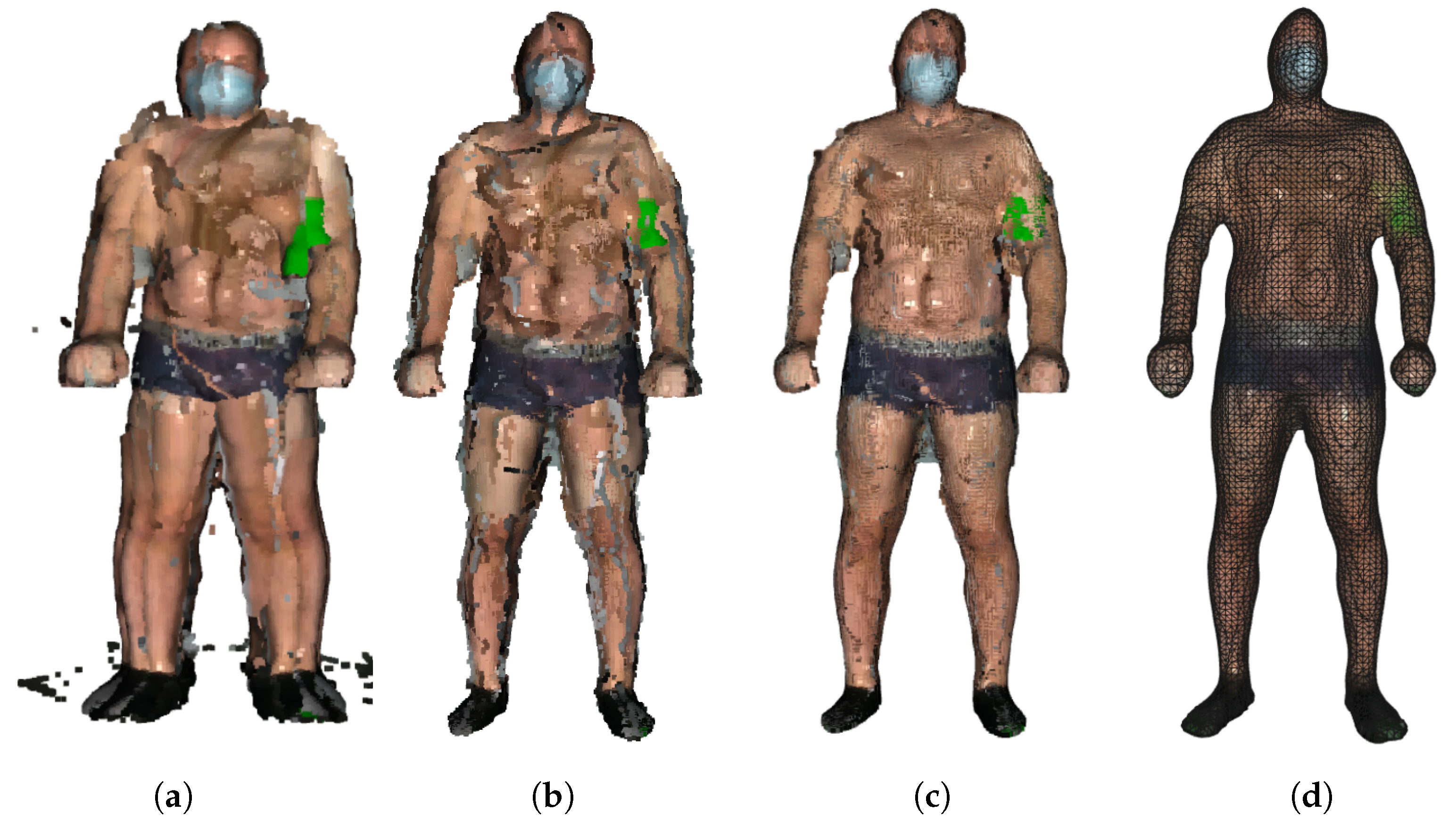
21]. The smoothing effect of the MLS algorithm is presented in
Figure 3.
When applying the MLS smoothing, the size of the neighborhood used for fitting has to be chosen carefully. The larger value produces a smoother surface, yet it deforms the true geometry. On the other hand, the low value can result in a weak smoothing effect. We use the neighborhood radius of 5 cm. Again, we chose this value empirically, so that the skin appears as a smooth surface, but the original geometry of the input point cloud is preserved.
The final step is to create a triangulated approximation (triangle mesh) of the human body surface, which is formed on the point cloud refined by the previous processing steps. We use the Poisson surface reconstruction (PSR) algorithm developed by Kazhdan et al. [
22] to reconstruct the surface from so-called oriented points (points with estimated normal vectors). It produces a watertight and smooth surface. PSR applies the marching cubes algorithm for surface extraction and stores the result in an octree of a given depth. An octree of depth D produces a three-dimensional mesh of maximal resolution
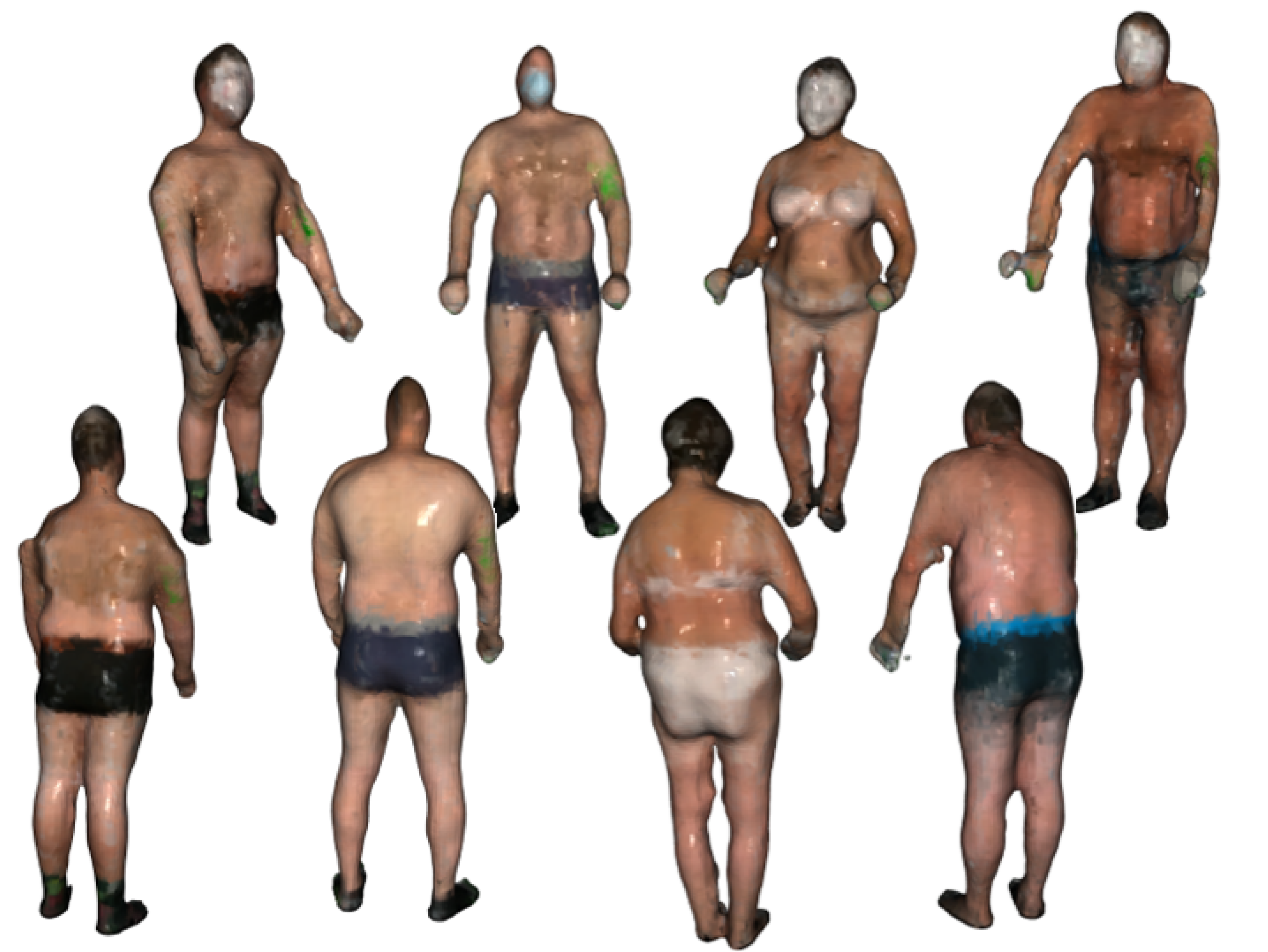
. Thus, as the octree depth increases, mesh resolution also increases. The higher depth value results in a detailed surface; however, it also emphasizes the remaining noise and artifacts. Choosing the lower value results in greater smoothing but lower details. We chose the depth of 7 as a trade-off between smoothness and resolution. The example final models of volunteers are presented in
Figure 4.
2.2. Texture Mapping
In principle, the models in
Figure 4 define the shape of the surface. For a more complete visualization, additional information about the color is superimposed on the models. It comes from the cameras built into the depth scanner. However, this color data is of low resolution and does not allow for the identification and analysis of nevi. For identification and analysis of nevi images, high-resolution cameras are used. However, as stated before, the individual nevi visible in the images are geometrically distorted and need to be orthorectified. This process requires information from the 3D model. Therefore, correspondences between the vertices of the model mesh and the coordinates of the corresponding locations in the high-resolution images must be found. By knowing these correspondences or relations and knowing coordinates on the surface of the model, one can find the corresponding fragment of the high-resolution image. On the other hand, by selecting a point in a high-resolution image, it is possible to find a corresponding location on the surface of the model.
In computer graphics, the process of finding the relations between coordinates in raster images and coordinates of vertices in the 3D mesh is called texture mapping. The high-resolution image, the texture, is superimposed on the triangle mesh to visualize the model with appropriate detail. In the case of our approach, a known fragment of the high-resolution image, which may present an individual nevus, is matched to the coordinates on the surface of the model. Since the coordinates of the camera at the time of taking the picture are known, the distance between the camera and the location of the nevus on the model can be calculated. Moreover, the model enables determination of the normal vector to the skin surface and, thus, the orientation of this surface in relation to the optical axis of the camera. These two pieces of information are sufficient to locally orthorectify the image at the point where the nevus is visible.
In the following, we formally explain how the texture mapping is carried out, and how the relations between high-resolution images and the 3D model are used to locally orthorectify the images.
Texture mapping is a process of finding relations between the vertices of the triangle mesh
and coordinates
in the texture image. It is accomplished by transforming the coordinates of every vertex from OCS to CCS. The transformation (Equation (
2)) is described by the matrix defining relative rotation of the object with respect to the arm by the angle
, and by the translation vector including camera elevation
above the floor level and distance
from the rotation axis. These make Equation (
2) similar to Equation (
1), which defines relations between DCS and OCS. However, the camera orientation may not be exactly as desired due to assembly imperfections. It can be mounted slightly askew or shifted. To account for these discrepancies, the calibration matrix
and the calibration vector
are introduced into the equation. The matrix and the vector should be determined individually for each camera as a result of the calibration procedure consisting of exact alignment of the texture images with the model.
After transforming the coordinates of the mesh vertices to the CCS, using the model of a pinhole camera, the vertex coordinates are projected onto the space of a two-dimensional texture image (Equation (
3)). The
parameter reflects the properties of the optical system of the camera and the resolution of the image sensor. As a result, we obtain coordinates in the texture image related to the vertices of the mesh.
It must be noted that there are many images of the human subject taken at various angles and by various cameras mounted at different heights above the floor level. Therefore, the computation defined by Equations (2) and (3) has to be repeated for all available texture images individually.
There are three practical problems with texturing. The first one is the occlusion of some body fragments by the other fragments which are closer to the camera, for example, armpit areas obscured by arms. This means that the fragment of the mesh related to the occluded fragment should not be textured with the particular texture image, as the texture does not picture this fragment. Secondly, the texture should not be mapped on parts of the model that are on the opposite side—not facing the camera lens. Finally, the third difficulty is that the same regions of the skin may be visible in several images taken by different cameras or at different angles. In this case, there is a need to decide which of the images presents the fragment with the greatest accuracy and therefore which of the images is the most appropriate for texturing the related fragment of the model.
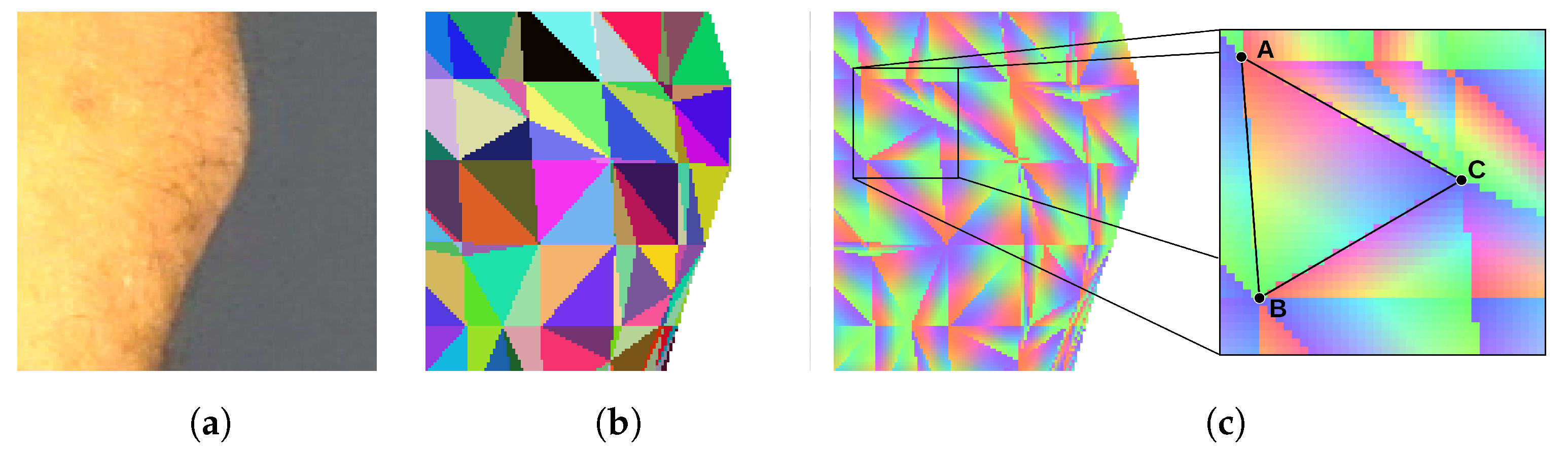
To determine if the particular triangle of the mesh should be textured by the particular piece of the image, we render the triangle mesh. The model is rendered as if it was visible from the point of view of the camera that has taken the texture image. Every triangle of the mesh is assigned a unique color for identification. Thus, the rendering result is an image consisting of a mosaic of colored triangles (
Figure 5b). The rendered surface should exactly align with the corresponding body fragment in the texture image, and the two images should be of the same size. Therefore, the pixel of the texture image which displays a particular point of the skin can be related to the particular triangle of the mesh by checking the color of the pixel at the same location in the rendered image.
The rendered image of a triangle mosaic can be quickly produced by means of the contemporary graphics processing units (GPUs). The GPUs run the back-face culling and the occlusion culling procedures to determine which areas of the rendered surface are not visible. Therefore, the resulting image does not show triangles, which are obscured or facing away from the camera lens. As the vertices of a triangle are being projected onto the texture image, with Equations (2) and (3), we verify if the particular triangle is visible in the mosaic. If the color of the triangle in the mosaic does not match the projected one, then the particular texture is not assigned to the triangle. This way, comparison of the mosaic image with the texture image enables determination of obscured skin fragments and solves the first two difficulties.
In a multicamera system, the same triangle may be textured with information from several images obtained from various cameras or at different angles. In our approach for texturing the triangle, we select the image which presents the particular skin fragment with the highest resolution. Therefore, after projecting the triangle vertices onto the texture image, we establish the area of the projected triangle. Then, we select the image for which the area is the largest. This solves the third difficulty.
The model with superimposed images of the skin surface serves multiple purposes. It enables visualization of the human body, localization of a skin nevus on its surface, and retrieval of the information on the distance and orientation of the skin fragment. When viewing, the user can rotate or change the size of the model, and indicate a specific place on its surface, for example, a mole that he or she wants to analyze. The user should be able to immediately see the original image or orthorectified visualization of the indicated location. The other scenario is image segmentation and automatic nevi detection in texture images. After detecting the nevus in the image, it is also necessary to retrieve the information from the model needed for orthorectification.
Identification of the place indicated by the user takes place in two stages. We assume that the user observes the model at some chosen orientation and scale. This means that the textured model has been rendered in this orientation and is presented on the screen. By means of the mouse or a touch, the user indicates a particular point on the rendered image. Then, the algorithm renders the triangle mosaic image in the same scale and orientation as the model visible to the user. The algorithm checks the color of the mosaic image at the same location as indicated by the user. The color enables the identification of the corresponding triangle on the model’s mesh. This technique is known in computer graphics as mouse picking [
23,
24,
25].
In the second scenario, the input for the procedure are coordinates of the nevus identified by image processing. Again, the mosaic of triangles is rendered from the same point of view as the texture image was taken. The color of the mosaic taken from the same coordinates enables identification of the model’s triangle.
In both scenarios, identification of the triangle is not enough. Thus, in the next step, we render an image in which each triangle is linearly shaded with RGB color components (
Figure 5c). Each of the three vertices of the triangle is assigned one of the three color components. As the color over the surface of the triangle is interpolated, every point of the triangle has a unique color shade. It can be noticed that the proportions of color components at a specific location correspond with the barycentric coordinates of this location. As a result, the coordinates
of the indicated location are obtained as a sum of coordinates of the triangle vertices
,
, and
weighted by the color component proportions
r,
g, and
b (Equation (
4)).
The method explained in this section finds a link between a point in the texture image and the corresponding point on the model surface. This in turn provides data for further computation of the distance between the point and the camera and the local orientation of the surface. The method is time-efficient as it utilizes graphics processing units available on almost every computer, tablet, or smartphone, which are able to render images in a fraction of a second.
2.3. Image Reconstruction
Another application of the model is to obtain information about the distance and orientation of the skin surface in relation to the optical axis of the camera—the camera by which a high-resolution texture image was taken. This information is necessary to orthorectify the image from the camera. As explained in the previous section, the point indicated on the high-resolution texture image can be linked with the corresponding point and the corresponding triangle in the model’s triangle mesh.
We know the
coordinates of the center of a nevus. In the mosaic image, we read the color and identify the indicated triangle. From the image of the shaded triangles, we read the color components, convert them to barycentric coordinates, and calculate the coordinates of the center of the nevus in the OCS (Equation (
4)). Next, we calculate the normal vector
to the surface of the triangle (Equation (
5)), where
,
, and
are vectors of coordinates of the triangle vertices.
Let us consider an imaginary orthogonal camera which serves as a means to orthorectify the image of the nevi. The virtual camera coordinate system (VCS) is created in such a way (
Figure 1) that the camera is pointed at the
point. Its optical axis
is perpendicular to the surface of the model at this point and antiparallel to the normal vector n (Equation (
6)). We also assume that the
is parallel to the XZ plane of the OCS and perpendicular to the
(Equation (
7)). As the
is perpendicular to the
and
, we calculate its axis as a vector product of the two axes (Equation (
8)). Finally, we obtain Equation (
9) to transform the coordinates from the OCS to the VCS.
By having the coordinates in the VCS, we can project them onto the surface of the sensor of the virtual camera. The equation defining orthogonal projection of the
onto the surface of the orthorectified image takes the form of Equation (
10), where
s is an arbitrary scaling factor.
Equations (8) and (9) enable computation of the coordinates of a point in the corrected, orthorectified image on the basis of coordinates of this point in the OCS. However, when generating the corrected image, we usually have to solve the inverse problem. While knowing the coordinates
, we need to find coordinates on the surface of the model in the OCS and then coordinates
in the original texture image. To solve this problem, let us note that the matrix
in Equation (
8) is orthonormal. Therefore, the inverse matrix can be simply obtained by its transposition
. In addition, the center of the corrected image
corresponds to the point
on the model’s surface. As a result of these observations, we obtain the relationship of Equation (
11).
The image reconstruction procedure is based on the fact that for each point of the reconstructed image, we find its counterpart in the texture image. For this, we use Equation (
10), and then Equations (2) and (3). When coordinates are found, the color components at the point
are interpolated. It should be noted that changing the scaling factors enables adjustment of the resolution of the resulting image in pixels per unit length. When knowing the resolution of the corrected image, the size of the nevi in the length units can be computed.
2.4. Experiment
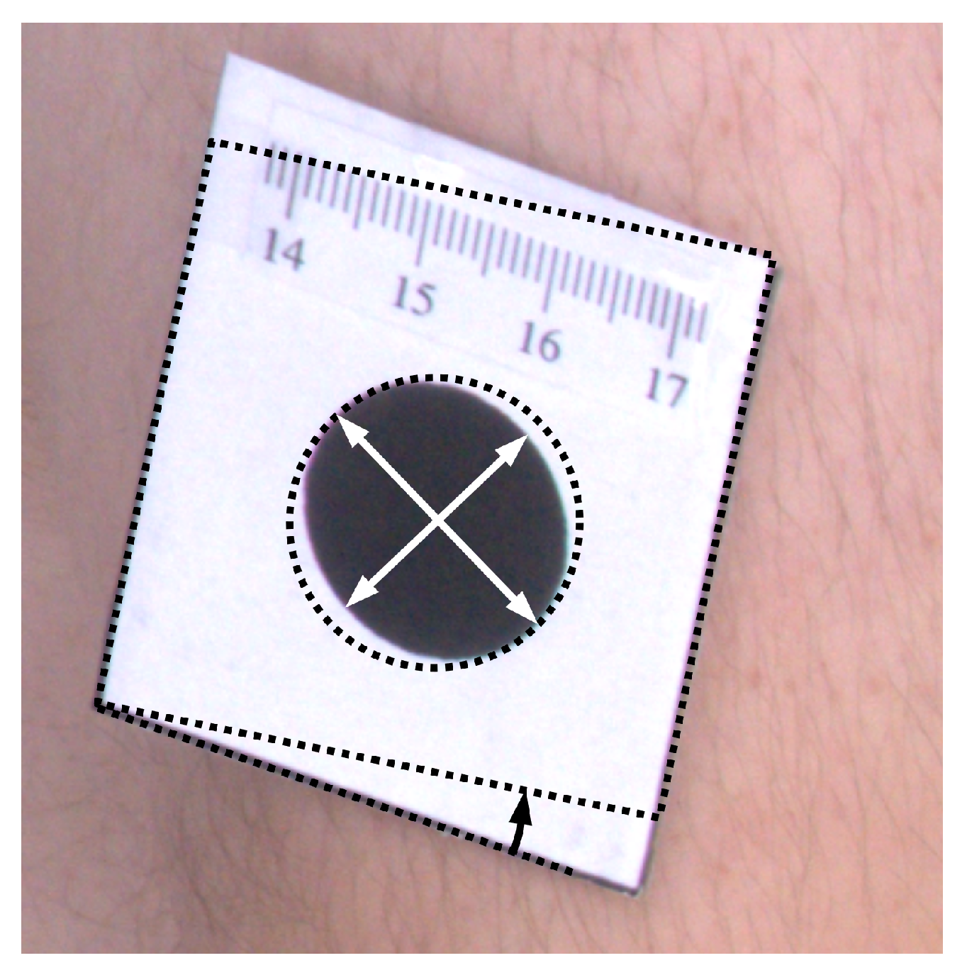
To assess the feasibility of image orthorectification with the presented method, we performed the following experiment. A volunteer with markers stuck to his skin was scanned. Every marker shows a black circle of 2 cm diameter. The volunteer was scanned using a prototype device consisting of the rotating arm with four Sony DSC RX100 cameras and three Intel RealSense D435 depth scanners. As the arm was turning, the images and point clouds were acquired at each subsequent 45 degree angle. The whole-body model was built, and the marker centers were indicated on the model. Next, the procedure for image orthorectification was applied.
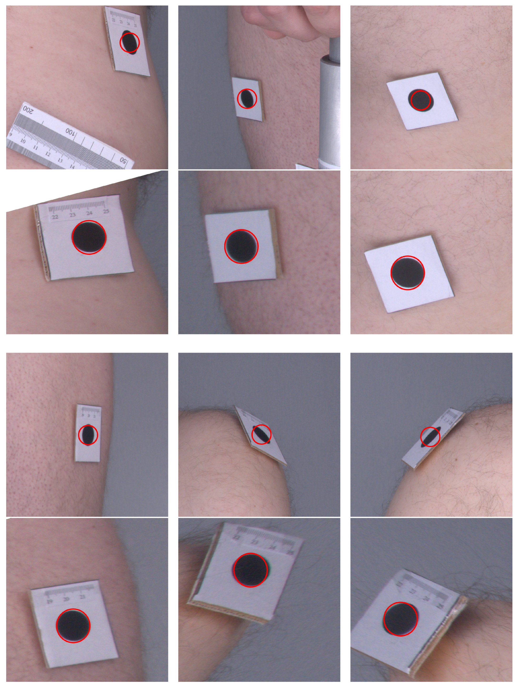
Figure 6 presents a comparison of the original images as they were acquired by the cameras and their corrected counterparts. One can see that, in the original images, the markers are elliptical in shape, and their sizes vary depending on their distance from the camera. In the corrected images, the markers are even in size and appear more similar to circles. The angles at the corners of the marker images also move closer to the right angle after applying the orthorectification procedure. Therefore, the visual inspection and comparison of the original and corrected images confirm that the orthorectification meets the expectations, and the resulting images allow for a more accurate assessment of the size and proportions.
To quantitatively assess results of orthorectification (
Figure 7), the ellipse was fitted to every marker, and proportions of semi-major to semi-minor axes were calculated. For such correctly rectified images, the proportion should be equal to one. Moreover, the area of the markers was computed, which for the circle of 2 cm diameter should be equal to
cm
. Furthermore, the shape of the tag that contains the marker is rectangular. Therefore, measuring the angle between the two edges of the tag and computing the difference between the angle and the right angle also facilitates the assessment of the rectification accuracy. The mean values of such measurements are presented in
Table 1.
The resulted values of the morphological attributes are closer to the desired ones after the images were orthorectified. The shear angle was reduced more than two times. The ratio of the semi-major to semi-minor axes is closer to one, with the error of the ratio reduced 2.7 times. The standard deviations of the area computations decreased almost two times, and the estimates of the area match the expected value.
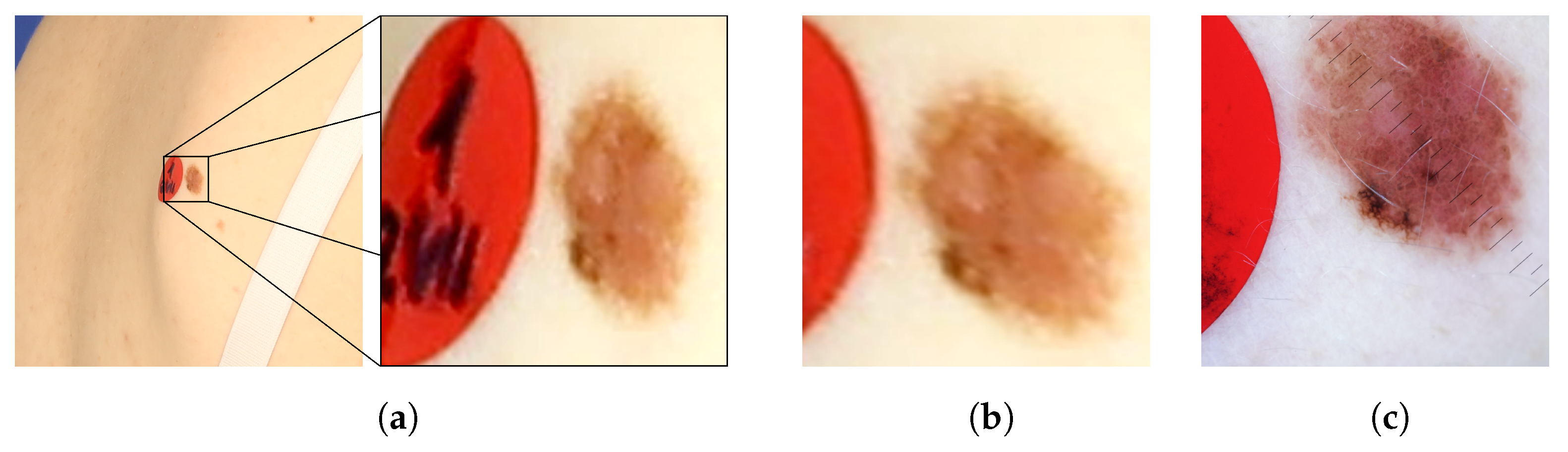
Figure 8 presents images of an exemplary noncancerous nevus. In the original image, the nevus’s proportions are distorted. Moreover, it is impossible to judge its actual size and the proportion of length to width. In the orthorectified image, the assessment of these morphological features becomes possible. For comparison, a reference image obtained with a dermatoscope is also presented. The shape and size of the corrected and reference images are similar.
It should be noted that the results were obtained with an imperfect 3D model of the human body. The surface of the model is not as smooth as in a real human body. There are apparent errors in the orientations of the model triangle faces, which contribute to the errors in orthorectified images. Building a model that reproduces the shape of the skin more accurately would, even more, improve the outcomes of the orthorectification procedure.


