RBFNN Design Based on Modified Nearest Neighbor Clustering Algorithm for Path Tracking Control


Abstract
:1. Introduction
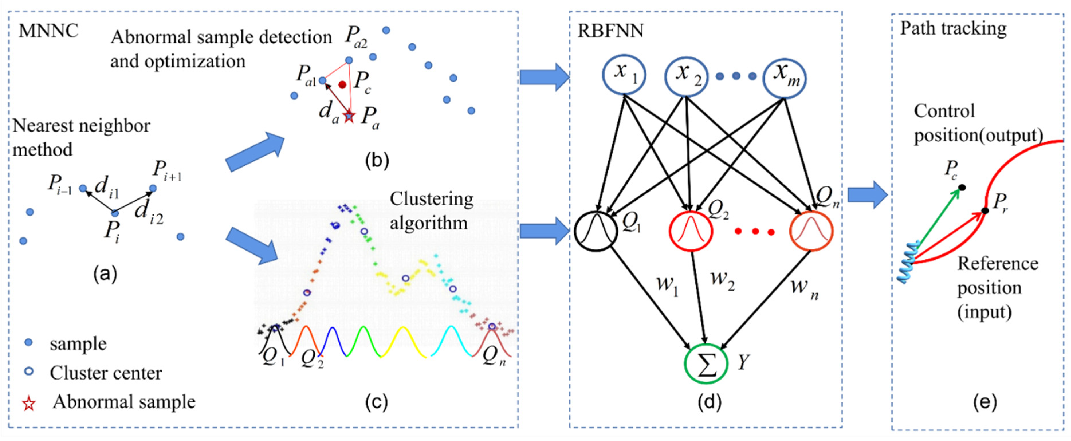
2. Concept of RBFNN Algorithm Based on MNNC for Path Tracking
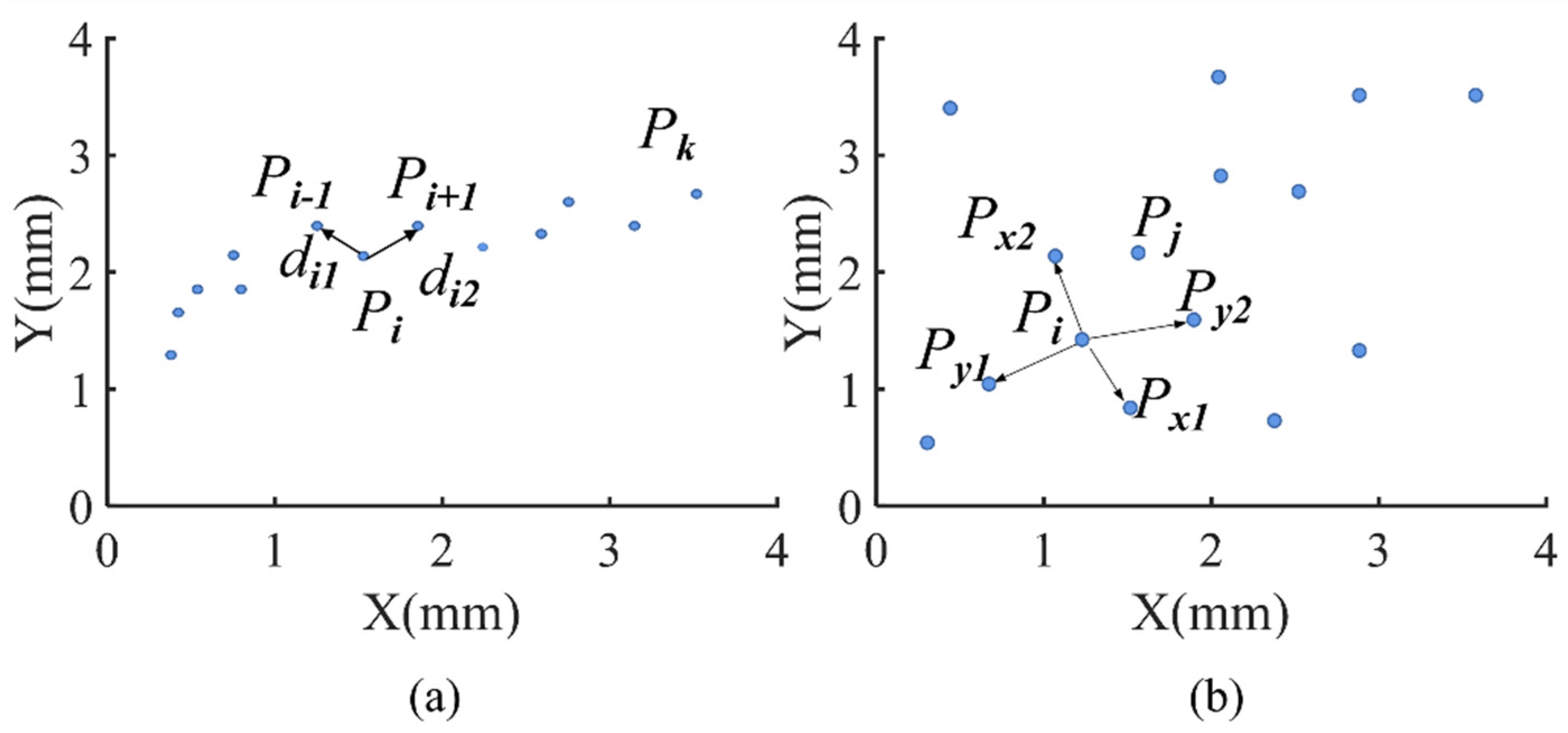
3. Clustering Algorithm Based on Nearest Neighbor
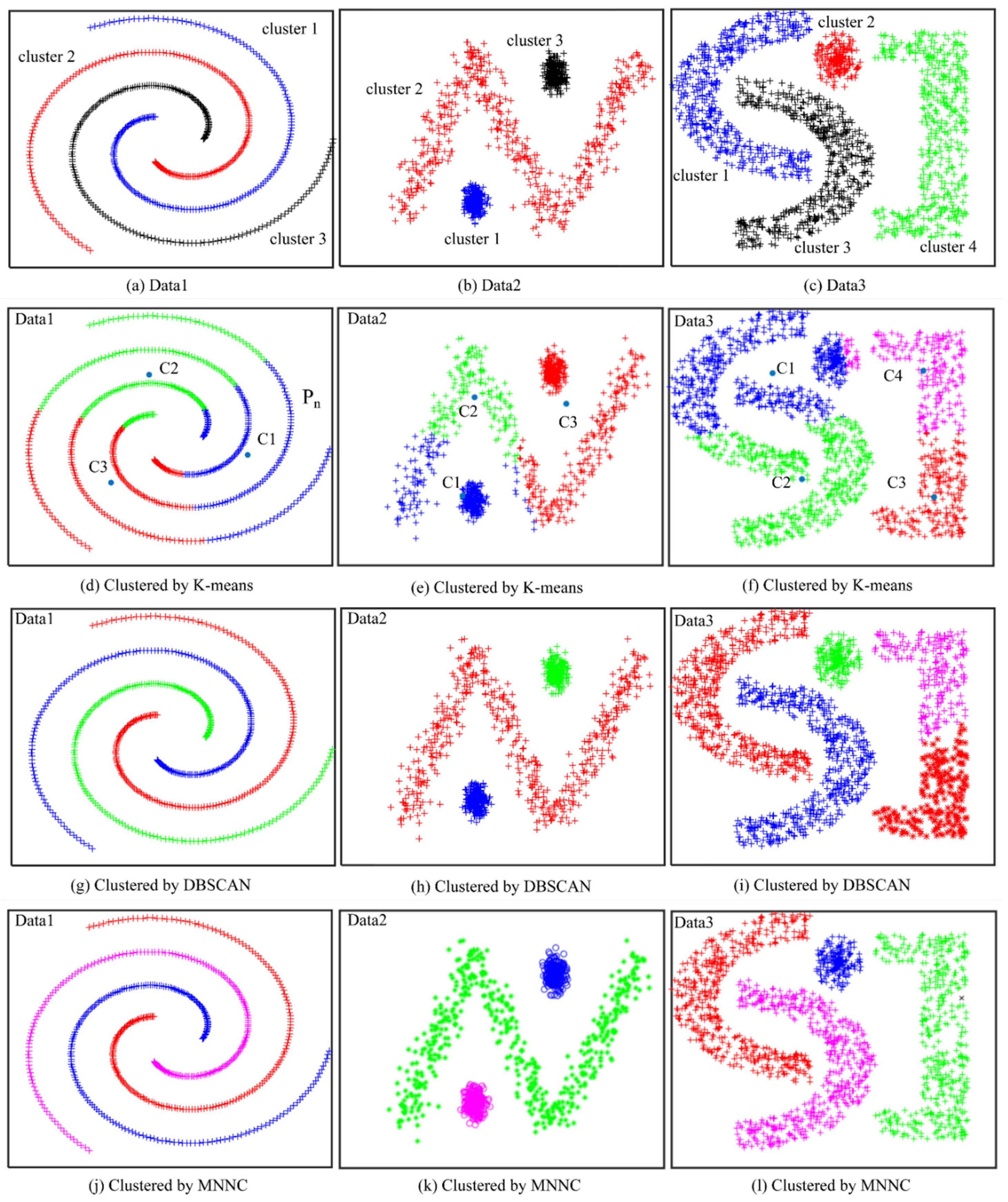
3.1. Typical Clustering Algorithm
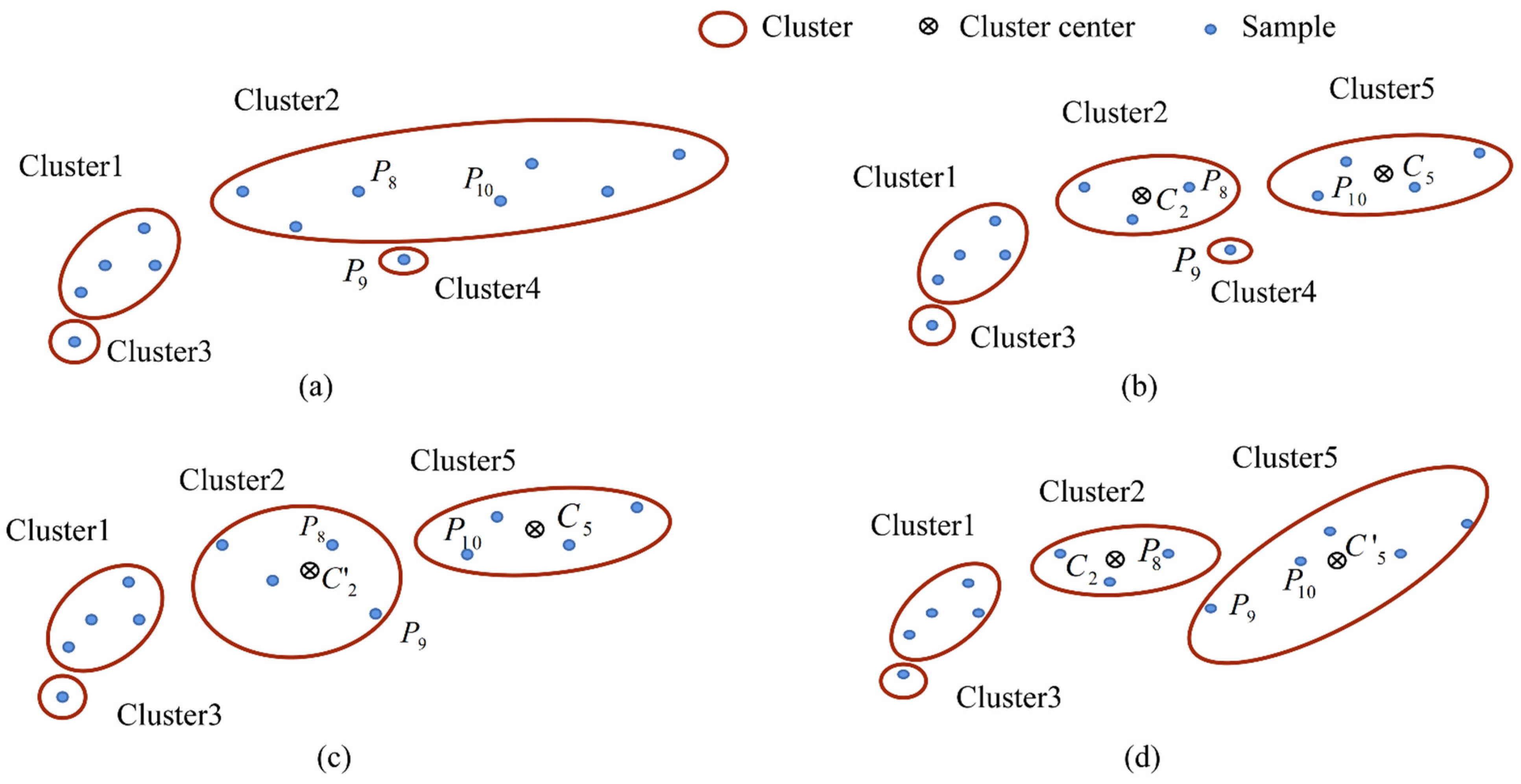
3.2. Modified Nearest Neighbor-Based Clustering Algorithm for Training RBFNN
| Algorithm 1. MNNC. |
| Input: training samples (P1,P2,……Pk), minimum samples number (Nmin) of cluster. |
| Output: clustering result |
| 1. for each sample Pi do |
| 2. Calculate the di of Pi; // referring to Definition 1. |
| 3. end for |
| 4. for each sample Pi do // arrange the samples into clusters referring to the distance. |
| 5. if di < dmin + dstep then Pi ∈cluster1; // Definition 2 |
| 6. else if di < dmin + 2 × dstep then Pi ∈cluster2; |
| 7. else if di < dmin + 3 × dstep then Pi ∈cluster3; |
| 8. else Pi ∈cluster4; |
| 9. end if; end for |
| 10. for cluster(i) do // The clusters with discontinuous sample numbers are divided into two clusters at the discontinuity. |
| 11. if the samples label of cluster(i) is not continuous then |
| 12. Divide the cluster(i) into cluster(i1) and cluster(i2) whose samples label is continuous. |
| 13. end if; end for |
| 14. for cluster(i) do // merge the small cluster into the adjacent clusters referring to Definition 3. |
| 15. if samples number of cluster(i) < Nmin then |
| 16. if ΔDi−1 < ΔDi+1 then cluster(i − 1) = cluster(i − 1) + cluster(i); |
| 17. else cluster(I + 1) = cluster(I + 1) + cluster(i); |
| 18. end if; end for |
| 19. Return clusters |
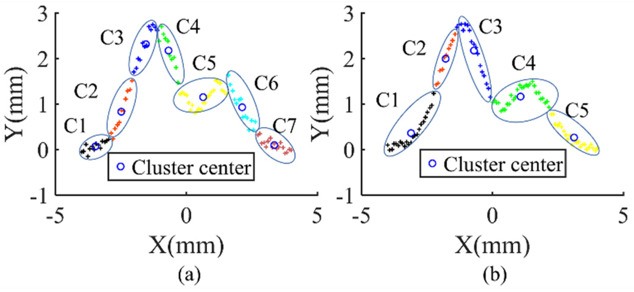
3.3. Enhancement of MNNC Performance
| Algorithm 2. MNNC for the path tracking of magnetic microrobot. |
| Input: training samples (P1,P2,……Pk). |
| Output: clustering result. |
| 1. for each sample Pi do |
| 2. Calculate the di of Pi; // referring to Definition 4. |
| 3. end for |
| 4. dmax = max(d1,d2,……dk); dmin = min(d1,d2,……dk); |
| 5. dstep = (dmax + dmin)/H; //H is distance level number that is determined by user. |
| 6. for each distance level; |
| 7. for each sample Pi do // find the nearest neighbors of Pi and establish the neighbor clusers. |
| 8. Find the smaple Pm which ‖Pm−Pi‖ ≤ dmin + H × dstep; |
| 9. Construct cluster(i) = (Pi, Pm); |
| 10. end for |
| 11. for each cluster(i) do // if clusters contain same sample, then merge these clusters into one cluster. |
| 12. If cluster(i) ∩ cluster(j) ≠ Ø then cluster(i) = cluster(i) + cluster(j); |
| 13. end if; end for |
| 14. end for |
| 15. merge the small cluster into nearest cluster |
| 16. Return clusters |
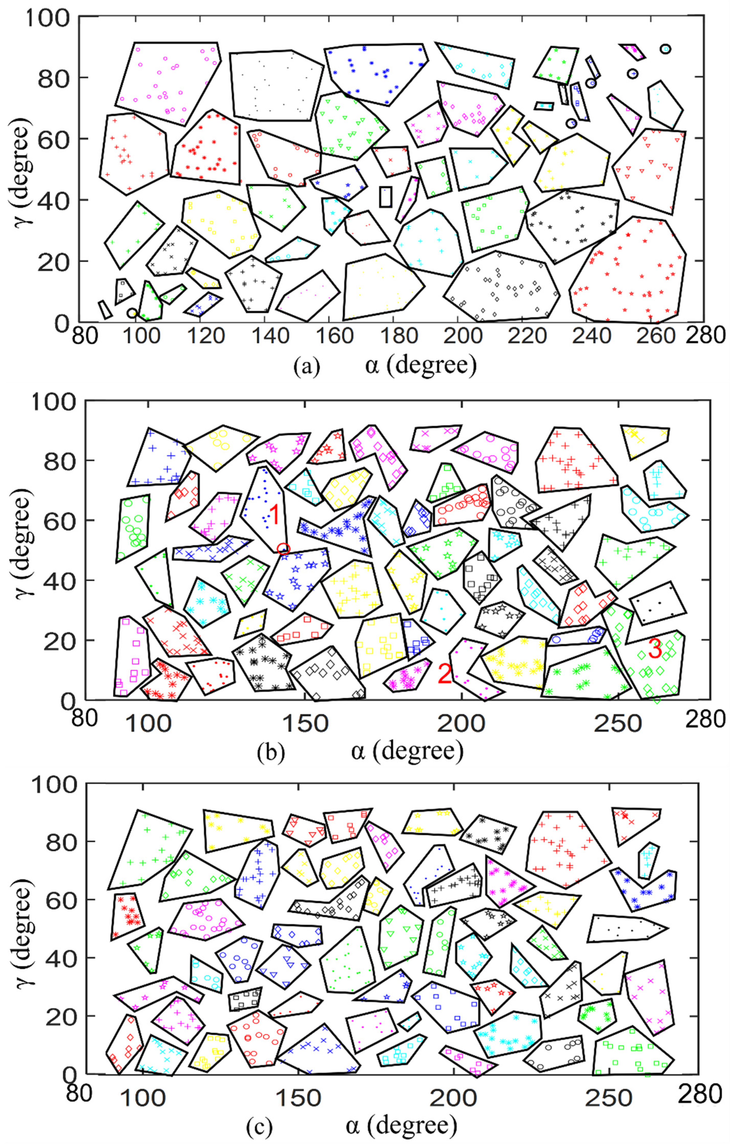
4. Adjustment of Training Samples Based on MNNC
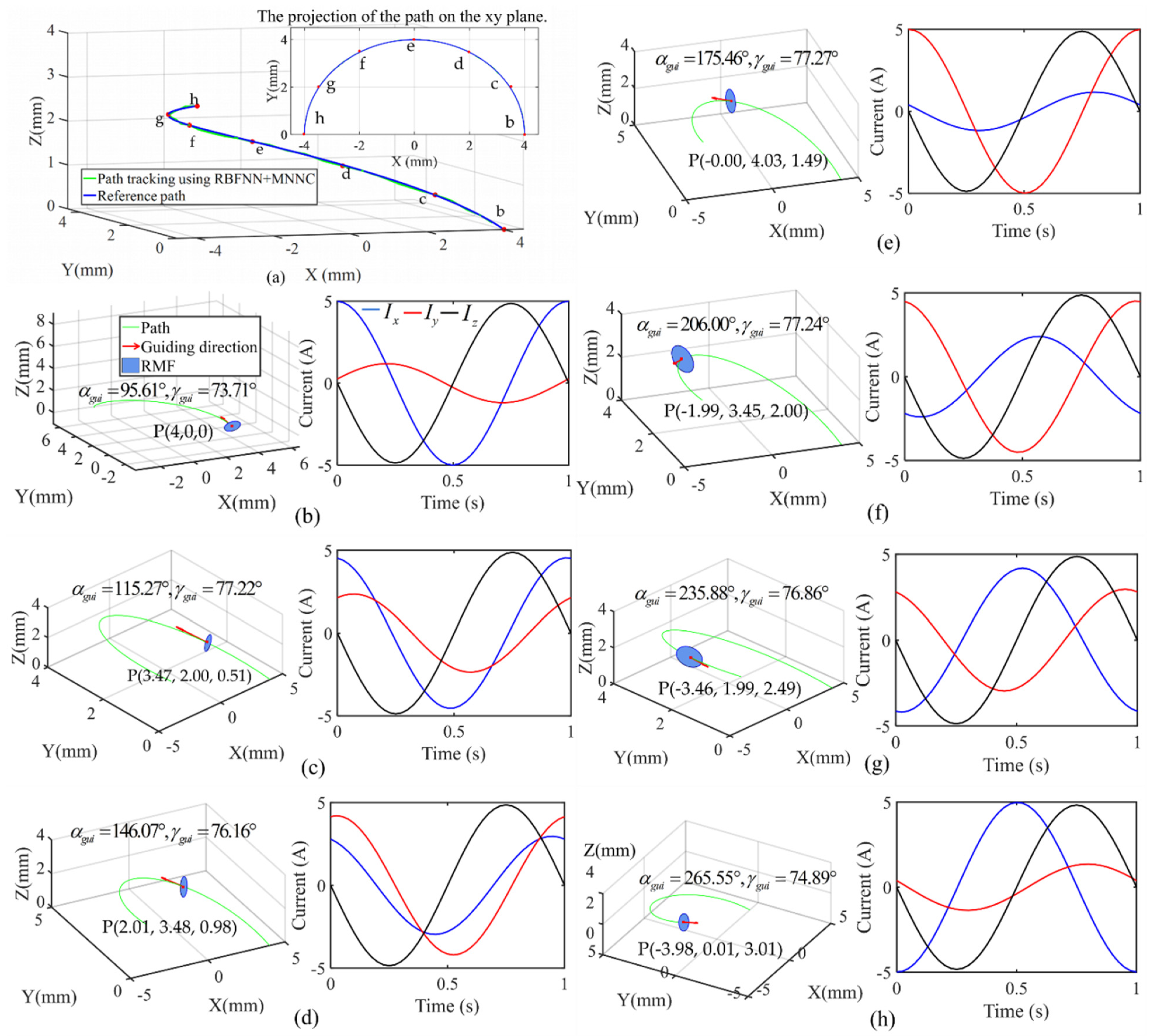
5. Application of RBFNN in Path Tracking for a Spiral-Type Magnetic Microrobot
6. Discussion
7. Conclusions
Author Contributions
Funding
Institutional Review Board Statement
Informed Consent Statement
Data Availability Statement
Conflicts of Interest
Appendix A

| RBFNN | Radial basis function neural network |
| MNNC | Modified nearest neighbor-based clustering |
| PID | Proportion integral differential |
| SVM | Support vector machines |
| GA | Genetic algorithm |
| AI | Artificial immune |
| DBSCAN | Density-based spatial clustering of applications with noise |
| DPC | Density peaks clustering |
| ACC | Accuracy |
| ADI | Adjusted Rand index |
| RMF | Rotating magnetic field |
| BIRCH | Balanced iterative reducing and clustering using hierarchies |
| CLIQUE | Clustering in QUEst |
Appendix B
| di | Distance between sample and its nearest neighbor |
| H | The number of di level |
| Pi | Sample |
| Distance change | |
| dstep | Distance step |
| D | Total distances between samples and centroid of cluster before merged |
| D’ | Total distances between samples and centroid of cluster after merged |
| Quani | Quantity of samples of cluster i |
| C | Center of cluster |
| R | Scanning radius of DBSCAN |
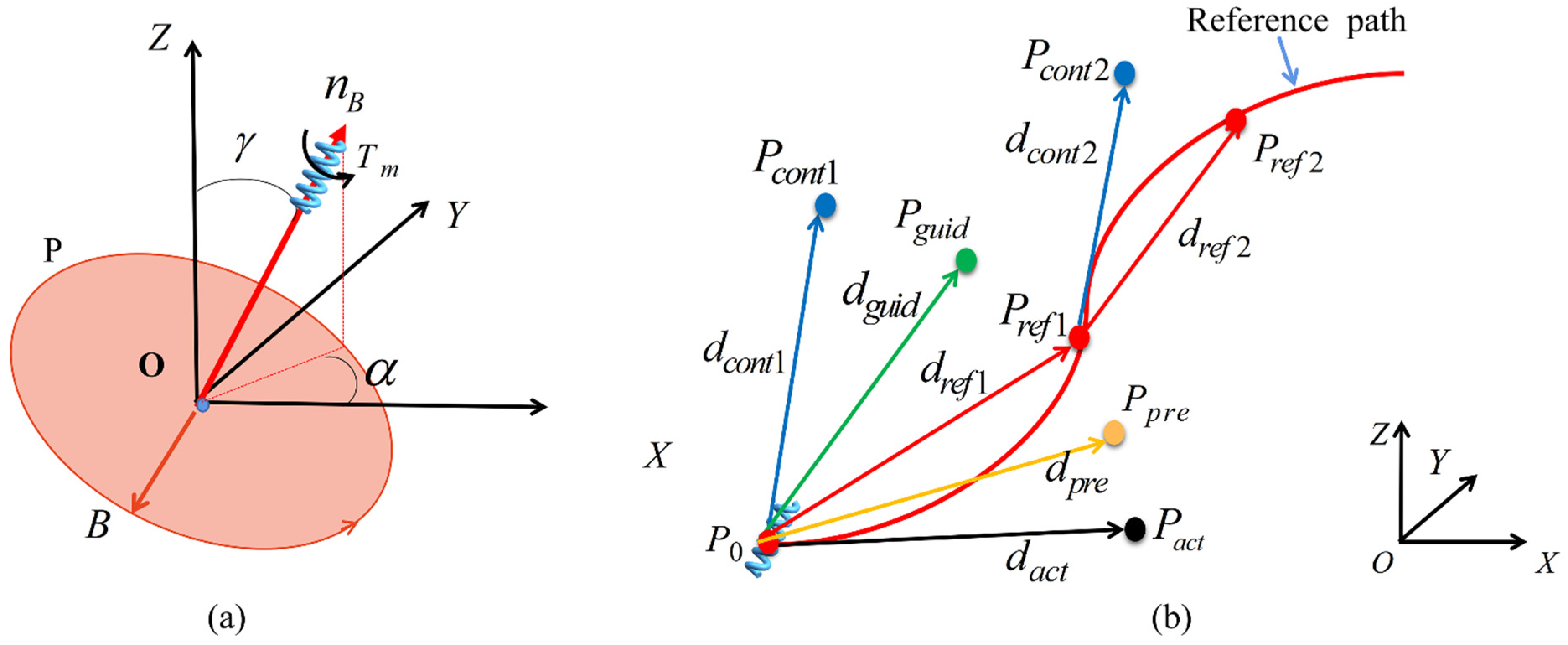
| Tm | Magnetic torque |
| V | Volume of microrobot |
| M | Magnetization of microrobot |
| B | External magnetic field |
| γ | Polar angle |
| α | Azimuthal angle |
| nB | Normal vector of plan P |
| Pcont | Control position |
| Pref | Reference position |
| Pact | Actual position |
| Pguid | Guidance position |
| Ppre | Predicted position |
| γref | Reference polar angle |
| αref | Reference azimuthal angle |
| γcont | Control polar angle |
| αcont | Control azimuthal angle |
| γguid | Guidance polar angle |
| αguid | Guidance azimuthal angle |
| γpre | Predicted polar angle |
| αpre | Predicted azimuthal angle |
| γcomp | Compensation of polar angle |
| αcomp | Compensation of azimuthal angle |
| dcont | Control direction |
| dguid | Guidance direction |
| dref | Reference direction |
| dpre | Predicted direction |
| dact | Actual direction |
| Qi | Output of hidden layer neuron of RBFNN |
| ci | Center of hidden layer neuron of RBFNN |
| wi | Weight between hidden layer and output layer of RBFNN |
| σ | Width of hidden layer neuron of RBFNN |
| μ0 | Permeability of free space |
| N | Turns number of coil |
| KB | Magnetic field coefficient of Helmholtz coil |
| I | Coil current |
| Ix | Coil current of x-axis |
| Iy | Coil current of y-axis |
| Iz | Coil current of z-axis |
| errgamma | Error of polar angle |
| erralpha | Error of azimuthal angle |
| errposition | Error of position |
References
- Rout, R.; Subudhi, B. Inverse optimal self-tuning PID control design for an autonomous underwater vehicle. Int. J. Syst. Sci. 2017, 48, 367–375. [Google Scholar] [CrossRef]
- Xiang, H.B.; Li, M.W.; Zhang, T.L.; Wang, S.J.; Zhang, M.; Song, Y.; Huo, W.X.; Huang, X. Motion characteristics of untethered swimmer with magnetoelastic material. Smart Mater. Struct. 2021, 30, 075030. [Google Scholar] [CrossRef]
- Ghosh, B.B.; Sarkar, B.K.; Saha, R. Realtime performance analysis of different combinations of fuzzy-PID and bias controllers for a two degree of freedom electrohydraulic parallel manipulator. Robot. Comput.-Integr. Manuf. 2015, 34, 62–69. [Google Scholar] [CrossRef]
- Algarin-Pinto, J.A.; Garza-Castanon, L.E.; Vargas-Martinez, A.; Minchala-Avila, L.I. Dynamic modeling and control of a parallel mechanism used in the propulsion system of a biomimetic underwater vehicle. Appl. Sci. 2021, 11, 4909. [Google Scholar] [CrossRef]
- Mai, T.A.; Dang, T.S.; Duong, D.T.; Le, V.C.; Banerjee, S. A combined backstepping and adaptive fuzzy PID approach for trajectory tracking of autonomous mobile robots. J. Braz. Soc. Mech. Sci. Eng. 2021, 43, 156. [Google Scholar] [CrossRef]
- Xu, B.J.; Ji, S.; Zhang, C.R.; Chen, C.; Ni, H.P.; Wu, X.J. Linear-extended-state-observer-based prescribed performance control for trajectory tracking of a robotic manipulator. Ind. Robot. 2021, 44, 544–555. [Google Scholar] [CrossRef]
- Li, Q.X.; Zhou, Y.S. Precise trajectory tracking control of ship towing systems via a dynamical tracking target. Mathematics 2021, 9, 974. [Google Scholar] [CrossRef]
- Wu, Y.; Wang, L.; Zhang, J.; Li, F. Path following control of autonomous ground vehicle based on nonsingular terminal sliding mode and active disturbance rejection control. IEEE Trans. Veh. Technol. 2019, 68, 6379–6390. [Google Scholar] [CrossRef]
- Liu, C.; Cheah, C.C.; Slotine, J. Adaptive Jacobian PID regulation for robots with uncertain kinematics and actuator model. In Proceedings of the 2006 IEEE/RSJ International Conference on Intelligent Robots and Systems, Beijing, China, 9–15 October 2006; pp. 3044–3049. [Google Scholar] [CrossRef]
- Smeresky, B.; Rizzo, A.; Sands, T. Optimal learning and self-awareness versus PDI. Algorithms 2020, 13, 23. [Google Scholar] [CrossRef] [Green Version]
- Juang, J.G. Intelligent trajectory control using recurrent averaging learning. Appl. Artif. Intell. 2001, 15, 277–296. [Google Scholar] [CrossRef]
- Chen, Z.; Yang, X.; Liu, X. RBFNN-based nonsingular fast terminal sliding mode control for robotic manipulators including actuator dynamics. Neurocomputing 2019, 362, 72–82. [Google Scholar] [CrossRef]
- Nie, L.; Guan, J.; Lu, C. Longitudinal speed control of autonomous vehicle based on a self-adaptive PID of radial basis function neural network. IET Intell. Transp. Syst. 2018, 12, 485–494. [Google Scholar] [CrossRef]
- Lee, C.T.; Tsai, C.C. Improved nonlinear trajectory tracking using RBFNN for a robotic helicopter. Int. J. Robust Nonlinear Control 2010, 20, 1079–1096. [Google Scholar] [CrossRef]
- Li, J.; Wang, J.; Wang, S. Neural approximation-based model predictive tracking control of non-holonomic wheel-legged robots. Int. J. Control Autom. Syst. 2020, 19, 372–381. [Google Scholar] [CrossRef]
- Guillen, A.; Rojas, I.; Gonzalez, J. Output value-based initialization for radial basis function neural networks. Neural Process. Lett. 2007, 25, 209–225. [Google Scholar] [CrossRef]
- Juang, J.G. Effects of Using Different Neural Network Structures and Cost Functions in Locomotion Control. In Lecture Notes in Computer Science, Proceedings of the 2nd International Conference on Natural Computation (ICNC 2006), Xian, China, 24–28, September 2006; Springer: Berlin/Heidelberg, Germany, 2006. [Google Scholar] [CrossRef]
- Fernandez-Navarro, F.; Hervas-Martinez, C.; Gutierrez, P.A. Generalised gaussian radial basis function neural networks. Soft Comput. 2013, 17, 519–533. [Google Scholar] [CrossRef]
- Huang, H.C.; Chiang, C.H. An evolutionary radial basis function neural network with robust genetic-based immunecomputing for online tracking control of autonomous Robots. Neural Process. Lett. 2016, 44, 19–35. [Google Scholar] [CrossRef]
- Chen, Z.Y.; Kuo, R.J. Combining SOM and evolutionary computation algorithms for RBF neural network training. J. Intell. Manuf. 2019, 30, 1137–1154. [Google Scholar] [CrossRef]
- Guillén, A.; Rojas, I.; Gonzalez, J. A possibilistic approach to RBFN centers initialization. In Lecture Notes in Computer Science, Proceedings of the 10th International Conference on Rough Sets, Fuzzy Sets, Data Mining and Granular Computing (RSFDGrC 2005), Regina, SK, Canada, 31 August 2005; Springer: Berlin/Heidelberg, Germany, 2005. [Google Scholar] [CrossRef]
- Oh, S.K.; Kim, W.D.; Pedrycz, W. Design of k-means clustering-based polynomial radial basis function neural networks (pRBF-NNs) realized with the aid of particle swarm optimization and differential evolution. Neurocomputing 2012, 78, 121–132. [Google Scholar] [CrossRef]
- Liao, C.C. Genetic k-means algorithm based RBF network for photovoltaic MPP prediction. Energy 2010, 35, 529–536. [Google Scholar] [CrossRef]
- Dogan, A.; Birant, D. Machine learning and data mining in manufacturing. Expert Syst. Appl. 2021, 166, 114060. [Google Scholar] [CrossRef]
- Fan, Y.K.; Bai, J.R.; Lei, X.; Lin, W.G.; Hu, Q.; Wu, G.D.; Guo, J.M.; Tan, G. PPMCK: Privacy-preserving multi-party computing for K-means clustering. J. Parallel Distrib. Comput. 2020, 154, 54–63. [Google Scholar] [CrossRef]
- Khalid, A.; Hammed, A. Genetic divergence in wheat genotypes based on seed biochemical profiles appraised through agglomerative hierarchical clustering and association analysis among traits. Pak. J. Bot. 2021, 53, 1281–1286. [Google Scholar] [CrossRef]
- Fang, X.J.; Wu, Y.J.; Liao, S.S.; Xue, L.Z.; Chen, Z.; Yang, J.N.; Lu, Y.M.; Ling, K.; Hu, S.Y.; Kong, S.Y. Division of crustal units in China using grid-based clustering and a zircon U-Pb geochronology database. Comput. Geosci. 2020, 145, 104570. [Google Scholar] [CrossRef]
- Montanari, G.E.; Doretti, M.; Marino, M.F. Model-based two-way clustering of second-level units in ordinal multilevel latent Markov models. Adv. Data Anal. Classif. 2021, 1–29. [Google Scholar] [CrossRef]
- Luo, S.; Liu, H.W.; Qi, E. Recognition and labeling of faults in wind turbines with a density-based clustering algorithm. Data Technol. Appl. 2021. [Google Scholar] [CrossRef]
- Li, C.Z.; Zhang, Y.Z. Density peak clustering based on relative density optimization. Math. Probl. Eng. 2020, 2020, 2816102. [Google Scholar] [CrossRef]
- Syarrudin, M.; Alfian, G.; Fitriyani, N.L. Performance analysis of IoT-based sensor, big data processing, and machine learning model for real-time monitoring system in automotive manufacturing. Sensors 2018, 18, 2946. [Google Scholar] [CrossRef] [Green Version]
- Minimol, P.V.; Mishra, D.; Gorthi, R.K.S.S. Guided MDNet tracker with guided samples. Visual Comput. 2021, 1–15. [Google Scholar] [CrossRef]
- Jeon, S.; Kim, S.; Ha, S.; Lee, S.; Kim, E.; Kim, S.Y.; Park, S.H.; Jeon, J.H.; Kim, S.W.; Moon, C. Magnetically actuated microrobots as a platform for stem cell transplantation. Sci. Robot. 2019, 4, eaav4317. [Google Scholar] [CrossRef]
- Chen, X.Z.; Hoop, M.; Mushtaq, S.F.; Hu, E.C.Z.; Nelson, B.J.; Pane, S. Recent developments in magnetically driven micro- and nanorobots. Appl. Mater. Today 2017, 9, 37–46. [Google Scholar] [CrossRef] [Green Version]
- Li, J.; Li, X. Development of a magnetic microrobot for carrying and delivering targeted cells. Sci. Robot. 2018, 3, eaat8829. [Google Scholar] [CrossRef] [PubMed] [Green Version]
- Yan, X.H.; Zhou, Q.; Vincent, M.; Deng, Y.; Yu, J.F.; Xu, J.B.; Xu, T.T.; Tang, T.; Bian, L.M.; Wang, Y.X.J.; et al. Multifunctional biohybrid magnetite microrobots for imaging-guided therapy. Sci. Robot. 2017, 2, eaaq1155. [Google Scholar] [CrossRef] [PubMed] [Green Version]
- Yang, C.; Wang, X.; Cheng, L. Neural-learning-based telerobot control with guaranteed performance. IEEE Trans. Cybern. 2017, 47, 3148–3159. [Google Scholar] [CrossRef] [PubMed] [Green Version]


| Clustering Algorithm | Performance Index | Dataset | ||
|---|---|---|---|---|
| Data 1 | Data 2 | Data 3 | ||
| K-means | ACC | 0.3333 | 0.6683 | 0.4891 |
| ARI | 0.0233 | 0.3121 | 0.3010 | |
| DBSCAN | ACC | 1 | 1 | 0.8558 |
| ARI | 1 | 1 | 0.9019 | |
| MNNC | ACC | 1 | 1 | 0.9994 |
| ARI | 1 | 1 | 0.9994 | |
| Curve Type | 2D Curve | 3D Curve | |
|---|---|---|---|
| Noise style | Randomly distributed | Six points with noise | Randomly distributed |
| Errors without adjustment | 3.0793 | 2.7281 | 516.6542 |
| Errors with adjustment | 2.8145 | 1.3292 | 485.3374 |
| Algorithm | Cluster Number | Training Error | Test Error |
|---|---|---|---|
| K-means | 59 | 2.27° | 2.89° |
| DBSCAN | 59 | 2.22° | 2.24° |
| MNNC | 59 | 2.10° | 2.21° |
| Position | Reference Angle (°) | Predicted Angle (°) | Angle Error Ratio (%) | Reference Coordinate (mm) | Predicted Coordinate (mm) | Position Error Ratio (%) | |||
|---|---|---|---|---|---|---|---|---|---|
| b | 93 | 76.57 | 93 | 76.57 | (4, 0, 0) | (4, 0, 0) | 0 | ||
| c | 117 | 76.57 | 115.78 | 75.79 | 1.04% | 1.02% | (3.46, 2.0, 0.5) | (3.47, 2.00, 0.51) | 2.48% |
| d | 147 | 76.57 | 144.40 | 79.89 | 1.77% | 4.34% | (2.0, 3.46, 1.0) | (2.01, 3.48, 0.98) | 7.31% |
| e | 177 | 76.57 | 172.34 | 77.90 | 2.63% | 1.74% | (0, 4.0, 1.5) | (−0.00, 4.03, 1.49) | 8.26% |
| f | 207 | 76.56 | 208.69 | 76.30 | 0.81% | 0.35% | (−2.0, 3.46, 2.0) | (−1.99, 3.45, 2.00) | 2.90% |
| g | 237 | 76.57 | 237.56 | 76.97 | 0.24% | 0.53% | (−3.46, 2.0, 2.5) | (−3.46, 1.99, 2.49) | 1.19% |
| h | 267 | 76.56 | 269.61 | 76.39 | 0.98% | 0.23% | (−4, 0, 3) | (−3.98, 0.01, 3.01) | 4.44% |
Publisher’s Note: MDPI stays neutral with regard to jurisdictional claims in published maps and institutional affiliations. |
© 2021 by the authors. Licensee MDPI, Basel, Switzerland. This article is an open access article distributed under the terms and conditions of the Creative Commons Attribution (CC BY) license (https://creativecommons.org/licenses/by/4.0/).
Share and Cite
Zheng, D.; Jung, W.; Kim, S. RBFNN Design Based on Modified Nearest Neighbor Clustering Algorithm for Path Tracking Control. Sensors 2021, 21, 8349. https://doi.org/10.3390/s21248349
Zheng D, Jung W, Kim S. RBFNN Design Based on Modified Nearest Neighbor Clustering Algorithm for Path Tracking Control. Sensors. 2021; 21(24):8349. https://doi.org/10.3390/s21248349
Chicago/Turabian StyleZheng, Dongxi, Wonsuk Jung, and Sunghoon Kim. 2021. "RBFNN Design Based on Modified Nearest Neighbor Clustering Algorithm for Path Tracking Control" Sensors 21, no. 24: 8349. https://doi.org/10.3390/s21248349
APA StyleZheng, D., Jung, W., & Kim, S. (2021). RBFNN Design Based on Modified Nearest Neighbor Clustering Algorithm for Path Tracking Control. Sensors, 21(24), 8349. https://doi.org/10.3390/s21248349