
DCNet: Densely Connected Deep Convolutional Encoder–Decoder Network for Nasopharyngeal Carcinoma Segmentation


Abstract
:1. Introduction
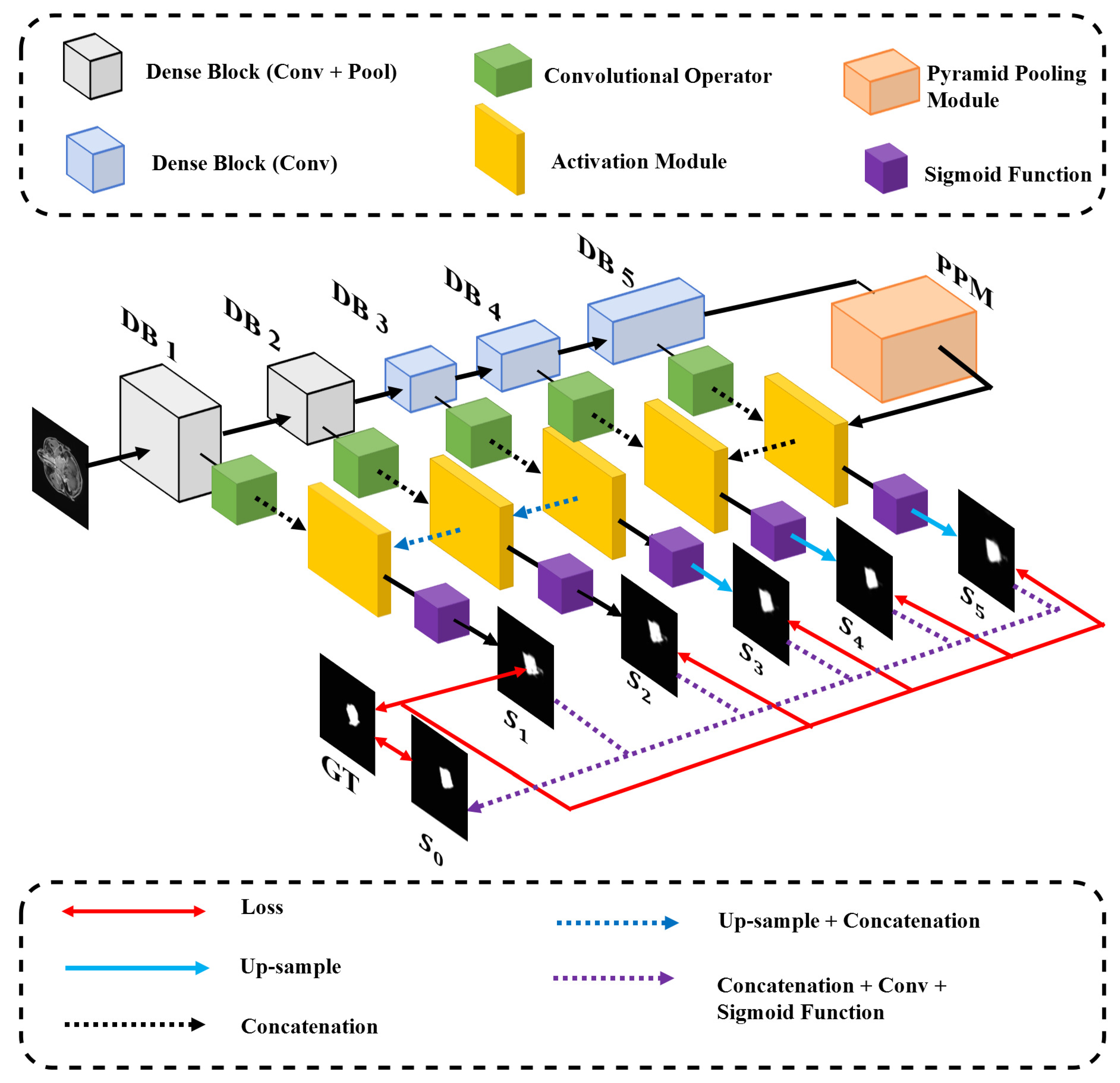
- We proposed a deep densely connected convolutional network with a pyramid pooling module followed to establish a multi-level representation of multi-scale feature maps. The size of GTV probably changes dramatically as the z-axis of the transverse slice changes. To remedy the large-scale variation, we deploy five densely connected convolutional blocks with expansive receptive fields to detect multi-scale regions of tumors and leverage a pyramid pooling module to fuse the information from different levels. The high-level feature maps with larger receptive fields contribute to locating tumors, and the low-level feature maps with smaller receptive fields with more spatial information contribute to refining segmentation.
- We involved and modified skip-connection architecture to our network and brought three-fold benefits: the relatively low-level spatial information is propagated to the corresponding level in the decoder network; the feature maps from the decoder network are convoluted before concatenation which outperforms direct concatenation; the convolutional layers added to compress the channels of feature maps to reduce the number of parameters and accelerate training steps.
- The multi-scale and multi-level loss functions contribute to realizing multi-scale supervision. It enhances the performance of multi-scale GTV detection.
2. Related Work
2.1. Traditional Methods
2.2. Deep Learning Methods
3. Methodology
3.1. Preprocessing
3.2. Network Architecture
3.2.1. The Encoder Network
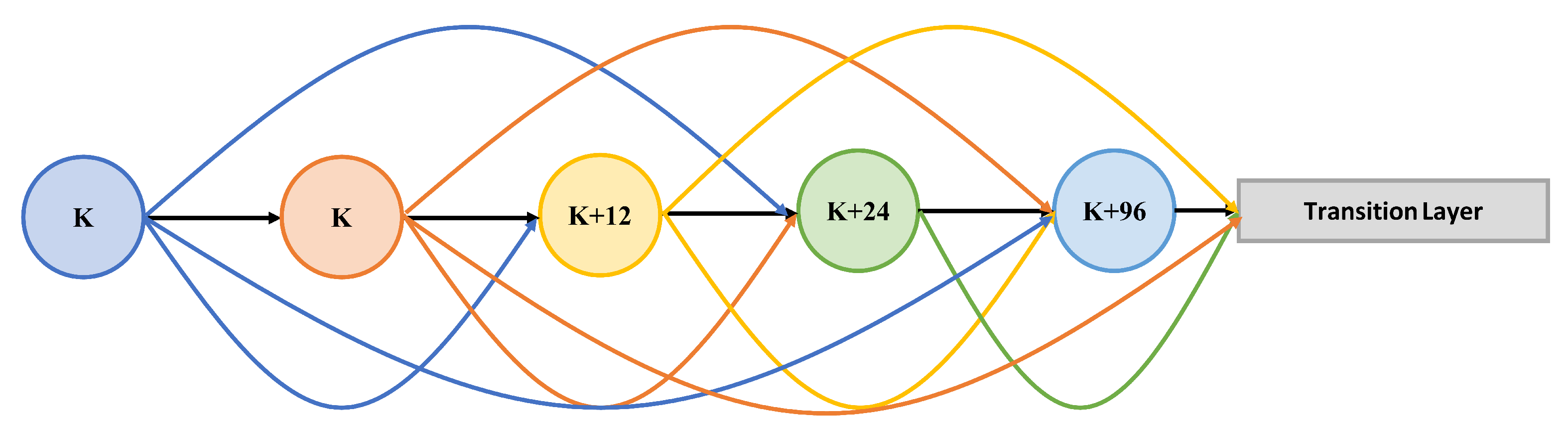
Dense Block

Skip-Connection
3.2.2. The Decoder Network
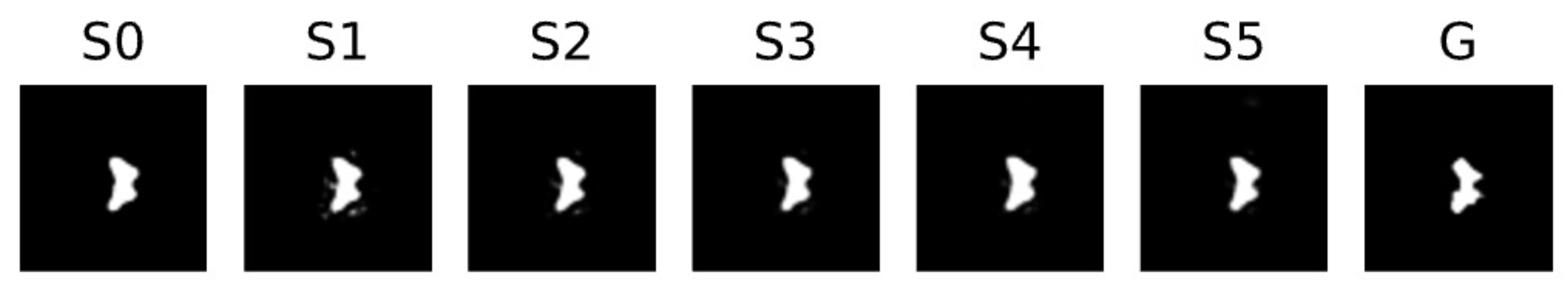
3.3. Multi-Level Integrated Loss Function
4. Experimental Evaluation
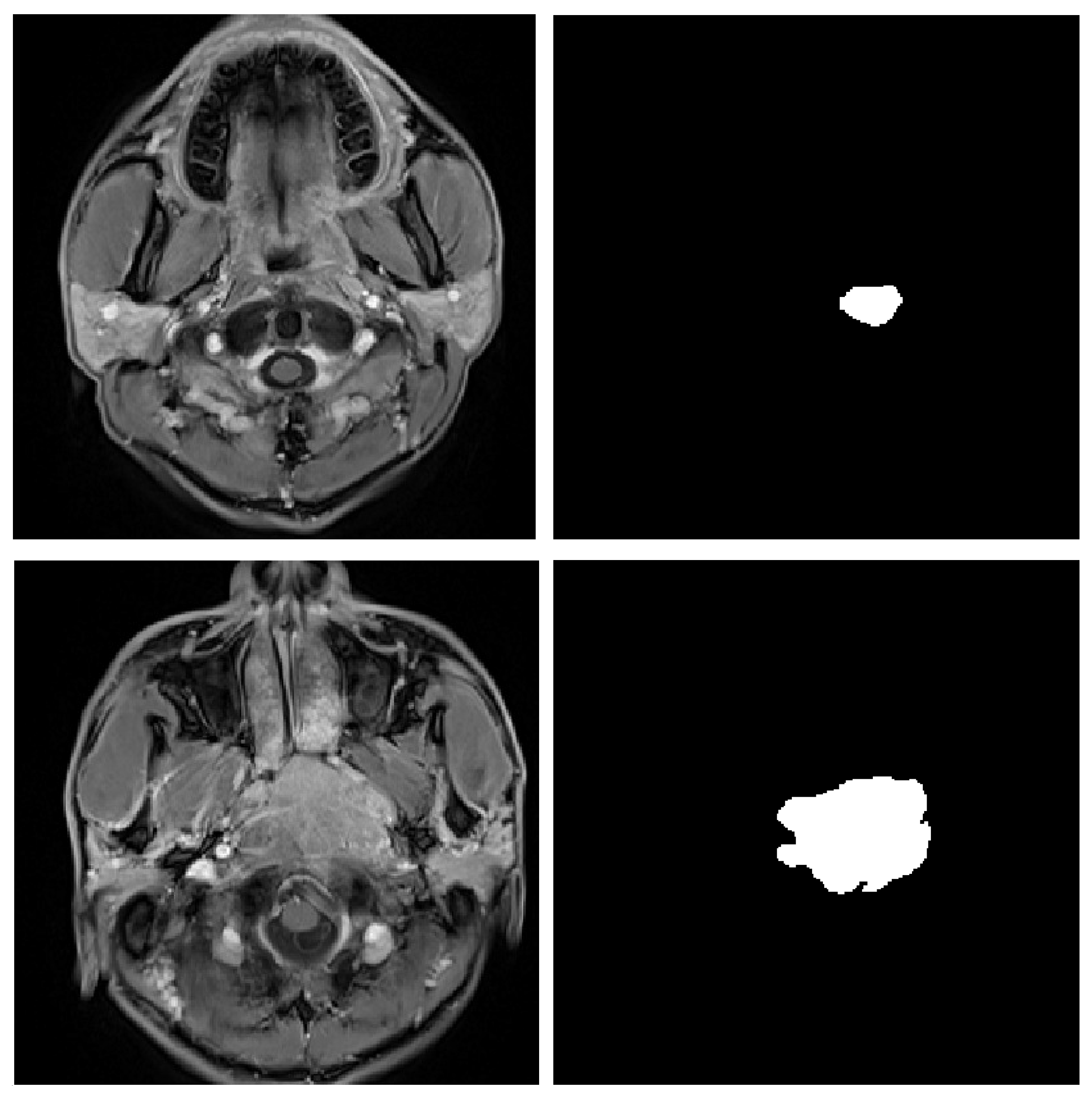
4.1. Data Acquisitions
4.2. Training Details
4.3. Experimental Results

| Net | DSC ↑ | SEN ↑ | SPE ↑ | PPV ↑ | VOE ↓ | RVD ↓ |
|---|---|---|---|---|---|---|
| U-Net [22] | 0.706 | 0.583 | 0.998 | 0.929 | 0.452 | 0.358 |
| U-Net++ [39] | 0.715 | 0.744 | 0.995 | 0.728 | 0.438 | 0.332 |
| FCN [38] | 0.742 | 0.732 | 0.996 | 0.767 | 0.405 | 0.139 |
| DCNet (ours) | 0.773 | 0.854 | 0.995 | 0.732 | 0.363 | 0.321 |
4.3.1. Sensitivity (SEN)
4.3.2. Specificity (SPE)
4.3.3. Positive Predictive Value (PPV)
4.3.4. Volumetric Overlap Error (VOE)
4.3.5. Relative Volume Difference (RVD)
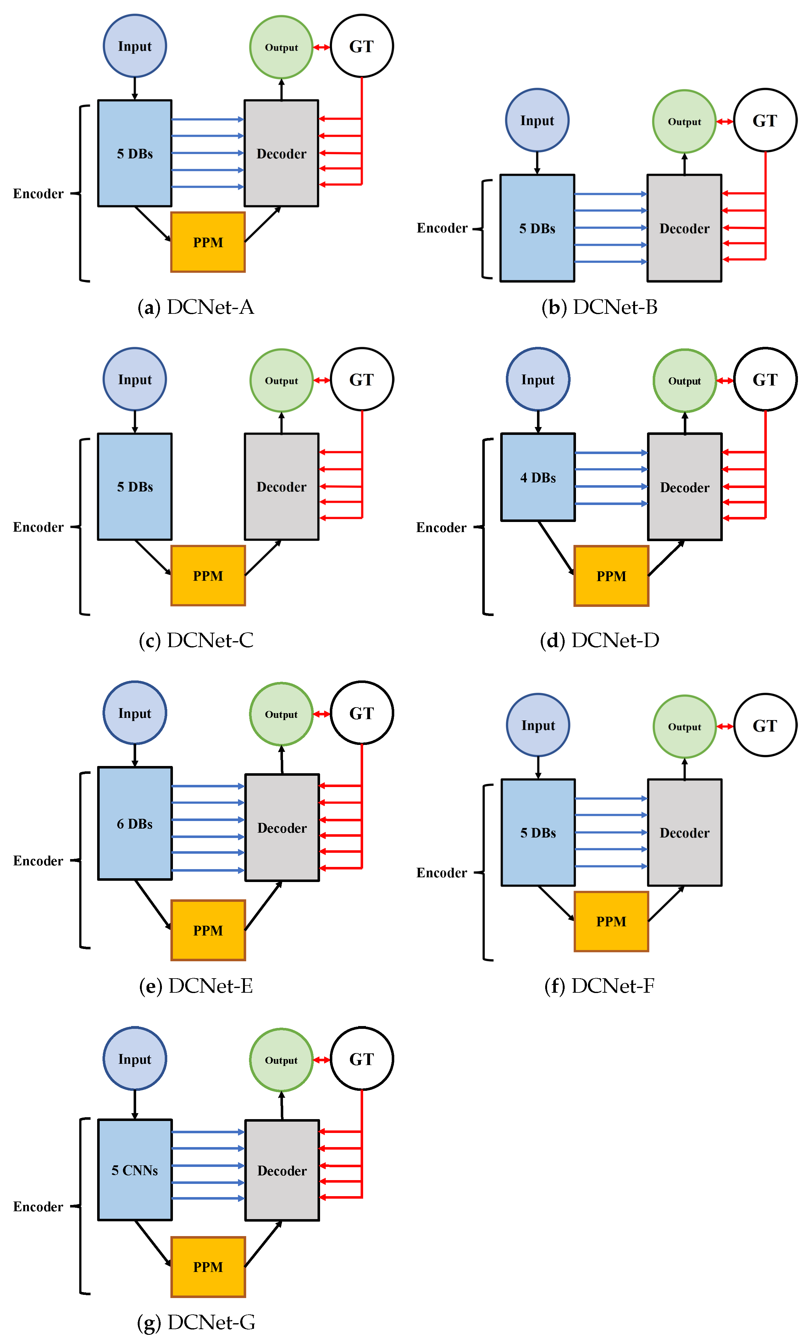
4.4. Ablation Analysis
4.4.1. Effectiveness of Key Modules of DCNet
Pyramid Pooling Module
Skip-Connection Architecture
Integrated Loss Function
The Number of Dense Blocks
Dense Block
4.4.2. Comparison of the Influence of Modules
5. Conclusions and Future Work
- 1.
- The influence of the value set of the hyper-parameters has not been investigated.
- 2.
- The network only processes a single 2D slice at one time. So, we think the network can take 3D image series as inputs by redesigning parts of the network, to speed up the prediction.
- 3.
- We consider using transfer learning methods, by training the network on the other data containing other tumors in MR images, to solve the problem of few data.
- 4.
- We have noticed Generative Adversarial Network (GAN) is used in web data to resolve the class imbalance problem [42]. In addition, we suppose it is a potential way to resolve the problem of intraclass variation and lack of sufficient data in our research. We consider involving a GAN in the preprocessing stage.
- 5.
- 6.
- We doubt whether it performs well in cases with other types of tumors, and we plan to investigate in the future.
Author Contributions
Funding
Institutional Review Board Statement
Informed Consent Statement
Data Availability Statement
Conflicts of Interest
References
- Chen, Y.; Chan, A.; Le, Q.; Blanchard, P.; Sun, Y.; Ma, J. Nasopharyngeal Carcinoma. Lancet 2019, 394, 64–80. [Google Scholar] [CrossRef]
- Mao, Y.; Tang, L.; Chen, L.; Sun, Y.; Qi, Z.; Zhou, G.; Liu, L.; Li, L.; Lin, A.; Ma, J. Prognostic Factors and Failure Patterns in Non-metastatic Nasopharyngeal Carcinoma after Intensity-modulated Radiotherapy. Chin. J. Cancer 2016, 35, 103. [Google Scholar] [CrossRef] [Green Version]
- Pow, E.; Kwong, D.; McMillan, A.; Wong, M.; Sham, J.; Leung, L.; Leung, K. Xerostomia and Quality of Life after Intensity-modulated Radiotherapy vs. Conventional Radiotherapy for Rarly-stage Nasopharyngeal Carcinoma: Initial Report on a Randomized Controlled Clinical Trial. Int. J. Radiat. Oncol. Biol. Phys. 2006, 66, 981–991. [Google Scholar] [CrossRef]
- Das, I.; Moskvin, V.; Johnstone, P. Analysis of Treatment Planning Time among Systems and Planners for Intensity-modulated Radiation Therapy. J. Am. Coll. Radiol. 2019, 6–7, 514. [Google Scholar] [CrossRef] [PubMed]
- Dong, S.; Gao, Z.; Sun, S.; Wang, X.; Li, M.; Zhang, H.; Yang, G.; Liu, H.; Li, S. Holistic and Deep Feature Pyramids for Saliency Detection. In Proceedings of the 29th British Machine Vision Conference, BMVC 2018, Newcastle, UK, 3–6 September 2018; p. 67. [Google Scholar]
- Hesamian, M.; Jia, W.; He, X.; Kennedy, P. Deep Learning Techniques for Medical Image Segmentation: Achievements and Challenges. J. Digit. Imaging 2019, 32, 582–596. [Google Scholar] [CrossRef] [Green Version]
- Olaf, R.; Philipp, F.; Thomas, B. U-net: Convolutional Networks for Biomedical Image Segmentation. In Proceedings of the Medical Image Computing and Computer-Assisted Intervention, MICCAI 2015, Munich, Germany, 5–9 October 2015; pp. 234–241. [Google Scholar]
- Zhao, H.; Shi, J.; Qi, X.; Wang, X.; Jia, J. Pyramid Scene Parsing Network. In Proceedings of the 30th IEEE Conference on Computer Vision and Pattern Recognition, CVPR 2017, Honolulu, HI, USA, 21–26 July 2016; pp. 6230–6239. [Google Scholar]
- Fitton, I.; Cornelissen, S.; Duppen, J.; Steenbakkers, R.; Peeters, S.; Hoebers, F.; Kaanders, J.; Nowak, P.; Rasch, C.; Van Herk, M. Semi-automatic Delineation Using Weighted CT-MRI Registered Images for Radiotherapy of Nasopharyngeal Cancer. Med. Phys. 2011, 38, 4662–4666. [Google Scholar] [CrossRef] [PubMed]
- Cortes, C.; Vapnik, V. Support-vector Networks. Mach. Learn. 1995, 20, 273–297. [Google Scholar] [CrossRef]
- Zhou, J.; Chan, K.; Xu, P.; Chong, F. Nasopharyngeal Carcinoma Lesion Segmentation from MR Images by Support Vector Machine. In Proceedings of the 3rd IEEE International Symposium on Biomedical Imaging, ISBI 2006, Arlington, VA, USA, 6–9 April 2006; pp. 1364–1367. [Google Scholar]
- Huang, W.; Chan, K.; Zhou, J. Region-based Nasopharyngeal Carcinoma Lesion Segmentation from MRI Using Clustering and Classification-based Methods with Learning. J. Digit. Imaging 2013, 26, 472–482. [Google Scholar] [CrossRef] [PubMed] [Green Version]
- Tatanun, C.; Ritthipravat, P.; Bhongmakapat, T.; Tuntiyatorn, L. Automatic Segmentation of Nasopharyngeal Carcinoma from CT images: Region Growing Based Technique. In Proceedings of the 2nd International Conference on Signal Processing Systems, ICSPS 2010, Dalian, China, 5–7 July 2010; Volume 2, pp. 537–541. [Google Scholar]
- Huang, K.; Zhao, Z.; Gong, Q.; Zha, J.; Chen, L.; Yang, R. Nasopharyngeal Carcinoma Segmentation via HMRF-EM with Maximum Entropy. In Proceedings of the 37th Annual International Conference of the IEEE Engineering in Medicine and Biology Society, EMBC 2015, Milan, Italy, 25–29 August 2015; pp. 2968–2972. [Google Scholar]
- Xu, A.; Wang, L.; Feng, S.; Qu, Y. Threshold-Based Level Set Method of Image Segmentation. In Proceedings of the 3rd International Conference on Intelligent Networks and Intelligent Systems, ICINIS 2010, Shenyang, China, 1–3 November 2010; pp. 703–706. [Google Scholar]
- Chen, J.; Liu, S. A Medical Image Segmentation Method Based on Watershed Transform. In Proceedings of the 5th International Conference on Computer and Information Technology, CIT 2005, Shanghai, China, 21–23 September 2005; pp. 634–638. [Google Scholar]
- Ng, H.; Ong, S.; Foong, K.; Goh, P.; Nowinski, W. Medical Image Segmentation Using K-Means Clustering and Improved Watershed Algorithm. In Proceedings of the 6th IEEE Southwest Symposium on Image Analysis and Interpretation, SSIAI 2006, Denver, CO, USA, 26–28 March 2006; pp. 61–65. [Google Scholar]
- Sudha, S.; Jayanthi, K.; Rajasekaran, C.; Sunder, T. Segmentation of RoI in Medical Images Using CNN-A Comparative Study. In Proceedings of the 34th IEEE Region 10 Conference, TENCON 2019, Kochi, India, 17–20 October 2019; pp. 767–771. [Google Scholar]
- Badrinarayanan, V.; Kendall, A.; Cipolla, R. SegNet: A Deep Convolutional Encoder-Decoder Architecture for Image Segmentation. IEEE Trans. Pattern Anal. Mach. Intell. 2017, 39, 2481–2495. [Google Scholar] [CrossRef]
- Shelhamer, E.; Long, J.; Darrell, T. Fully Convolutional Networks for Semantic Segmentation. IEEE Trans. Pattern Anal. Mach. Intell. 2017, 39, 640–651. [Google Scholar] [CrossRef]
- Jiang, H.; Diao, Z.; Yao, Y. Deep Learning Techniques for Tumor Segmentation: A Review. J. Supercomput. 2021, 77. [Google Scholar] [CrossRef]
- Çiçek, Ö.; Abdulkadir, A.; Lienkamp, S.S.; Brox, T.; Ronneberger, O. 3D U-Net: Learning Dense Volumetric Segmentation from Sparse Annotation. In Proceedings of the Medical Image Computing and Computer-Assisted Intervention, MICCAI 2016, Athens, Greece, 17 October 2016; pp. 424–432. [Google Scholar]
- Men, K.; Chen, X.; Zhu, J.; Yang, B.; Zhang, Y.; Yi, J.; Dai, J. Continual Improvement of Nasopharyngeal Carcinoma Segmentation with Less Labeling Effort. Phys. Medica 2020, 80, 347–351. [Google Scholar] [CrossRef]
- Huang, H.; Lin, L.; Tong, R.; Hu, H.; Zhang, Q.; Iwamoto, Y.; Han, X.; Chen, Y.; Wu, J. UNet 3+: A Full-Scale Connected UNet for Medical Image Segmentation. In Proceedings of the 45th IEEE International Conference on Acoustics, Speech and Signal Processing, ICASSP 2020, Barcelona, Spain, 4–8 May 2020; pp. 1055–1059. [Google Scholar]
- Men, K.; Chen, X.; Zhang, Y.; Zhang, T.; Dai, J.; Yi, J.; Li, Y. Deep Deconvolutional Neural Network for Target Segmentation of Nasopharyngeal Cancer in Planning Computed Tomography Images. Front. Oncol. 2017, 7, 7–15. [Google Scholar] [CrossRef] [Green Version]
- Chen, H.; Qi, Y.; Yin, Y.; Li, T.; Liu, X.; Li, X.; Gong, G.; Wang, L. MMFNet: A Multi-modality MRI Fusion Network for Segmentation of Nasopharyngeal Carcinoma. Neurocomputing 2020, 394, 27–40. [Google Scholar] [CrossRef] [Green Version]
- Zhao, L.; Lu, Z.; Jiang, J.; Zhou, Y.; Wu, Y.; Feng, Q. Automatic Nasopharyngeal Carcinoma Segmentation Using Fully Convolutional Networks with Auxiliary Paths on Dual-Modality PET-CT Images. J. Digit. Imaging 2019, 32, 462–470. [Google Scholar] [CrossRef]
- Zhang, W.; Yang, G.; Zhang, N.; Xu, L.; Wang, X.; Zhang, Y.; Zhang, H.; Javier, D.; de Albuquerque, V.H.C. Multi-task Learning with Multi-view Weighted Fusion Attention for artery-specific calcification analysis. Inf. Fusion 2021, 71, 64–76. [Google Scholar] [CrossRef]
- Ma, Z.; Wu, X.; Zhou, J. Automatic Nasopharyngeal Carcinoma Segmentation in MR Images with Convolutional Neural Networks. In Proceedings of the International Conference on the Frontiers and Advances in Data Science, FADS 2017, Xi’an, China, 23–25 October 2017; pp. 147–150. [Google Scholar]
- Lin, L.; Dou, Q.; Jin, Y.; Zhou, G.; Tang, Y.; Chen, W.; Su, B.; Liu, F.; Tao, C.; Jiang, N.; et al. Deep Learning for Automated Contouring of Primary Tumor Volumes by MRI for Nasopharyngeal Carcinoma. Radiology 2019, 291, 677–686. [Google Scholar] [CrossRef] [PubMed]
- Gu, R.; Wang, G.; Song, T.; Huang, R.; Aertsen, M.; Deprest, J.; Ourselin, S.; Vercauteren, T.; Zhang, S. CA-Net: Comprehensive Attention Convolutional Neural Networks for Explainable Medical Image Segmentation. IEEE Trans. Med. Imaging 2021, 40, 699–711. [Google Scholar] [CrossRef] [PubMed]
- Dong, H.; Yang, G.; Liu, F.; Mo, Y.; Guo, Y. Automatic Brain Tumor Detection and Segmentation Using U-Net Based Fully Convolutional Networks. Commun. Comput. Inf. Sci. 2017, 723, 506–517. [Google Scholar]
- Huang, G.; Liu, Z.; Maaten, L.; Weinberger, K. Densely Connected Convolutional Networks. In Proceedings of the 30th IEEE Conference on Computer Vision and Pattern Recognition, CVPR 2017, Honolulu, HI, USA, 21–26 July 2016; pp. 2261–2269. [Google Scholar]
- Ioffe, S.; Szegedy, C. Batch Normalization: Accelerating Deep Network Training by Reducing Internal Covariate Shift. In Proceedings of the 32nd International Conference on Machine Learning, ICML 2015, Lille, France, 7–9 July 2015; pp. 448–456. [Google Scholar]
- Lopes, A.; Ribeiro, A.; Silva, C. Dilated Convolutions in Retinal Blood Vessels Segmentation. In Proceedings of the 6th IEEE Portuguese Meeting on Bioengineering, ENBENG 2019, Lisbon, Portugal, 22–23 February 2019; pp. 1–4. [Google Scholar]
- Dumoulin, V.; Visin, F. A Guide to Convolution Arithmetic for Deep Learning. arXiv 2016, arXiv:1603.07285. [Google Scholar]
- Lin, T.; Dollár, P.; Girshick, R.; He, K.; Hariharan, B.; Belongie, S. Feature Pyramid Networks for Object Detection. In Proceedings of the 30th IEEE Conference on Computer Vision and Pattern Recognition, CVPR 2017, Honolulu, HI, USA, 21–26 July 2016; pp. 936–944. [Google Scholar]
- Shen, H.; Wang, R.; Zhang, J.; McKenna, S. Boundary-Aware Fully Convolutional Network for Brain Tumor Segmentation. In Proceedings of the 20th Medical Image Computing and Computer-Assisted Intervention, MICCAI 2017, Quebec City, QC, Canada, 11–13 September 2017; pp. 433–441. [Google Scholar]
- He, Y.; Yu, X.; Liu, C.; Zhang, J.; Hu, K.; Zhu, H. A 3D Dual Path U-Net of Cancer Segmentation Based on MRI. In Proceedings of the 3rd IEEE International Conference on Image, Vision and Computing, ICIVC 2018, Chongqing, China, 27–29 June 2018; pp. 268–272. [Google Scholar]
- Tobias, H.; Bram, G.; Martin, S.; Yulia, A.; Volker, A.; Christian, B.; Andreas, B.; Christoph, B.; Reinhard, B.; György, B.; et al. Comparison and Evaluation of Methods for Liver Segmentation from CT Datasets. IEEE Trans. Med. Imaging 2009, 28, 1251–1265. [Google Scholar]
- Yu, L.; Chen, H.; Dou, Q.; Qin, J.; Heng, P. Automated Melanoma Recognition in Dermoscopy Images via Very Deep Residual Networks. IEEE Trans. Med. Imaging 2017, 36, 994–1004. [Google Scholar] [CrossRef] [PubMed]
- Hao, J.; Wang, C.; Yang, G.; Gao, Z.; Zhang, J.; Zhang, H. Annealing Genetic GAN for Imbalanced Web Data Learning. IEEE Trans. Multimed. 2021. [Google Scholar] [CrossRef]
- Valanarasu, J.; Oza, P.; Hacihaliloglu, I.; Patel, V. Medical Transformer: Gated Axial-Attention for Medical Image Segmentation. In Proceedings of the 24th Medical Image Computing and Computer Assisted Intervention, MICCAI 2021, Virtual, 27 September–1 October 2021; pp. 36–46. [Google Scholar]
- Gao, Y.; Zhou, M.; Metaxas, D. UTNet: A Hybrid Transformer Architecture for Medical Image Segmentation. In Proceedings of the 24th Medical Image Computing and Computer Assisted Intervention, MICCAI 2021, Virtual, 27 September–1 October 2021; pp. 61–71. [Google Scholar]


| Methods | DSC ↑ | SEN ↑ | SPE ↑ | PPV ↑ | VOE ↓ | RVD ↓ |
|---|---|---|---|---|---|---|
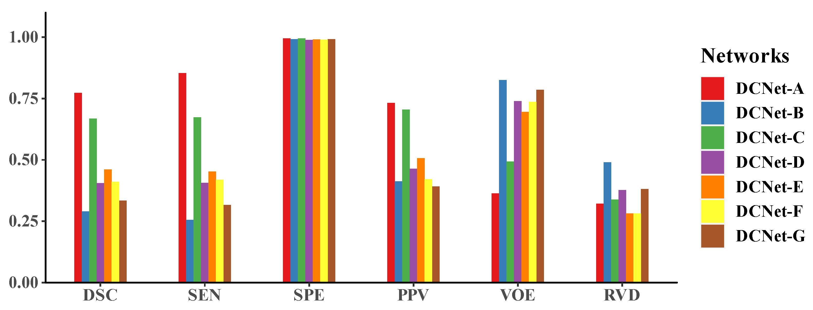
| DCNet-A (original) | 0.773 | 0.854 | 0.995 | 0.732 | 0.363 | 0.321 |
| DCNet-B (no PPM) | 0.290 | 0.255 | 0.992 | 0.412 | 0.825 | 0.490 |
| DCNet-C (no skip-connection) | 0.668 | 0.673 | 0.995 | 0.705 | 0.493 | 0.338 |
| Methods | DSC ↑ | SEN ↑ | SPE ↑ | PPV ↑ | VOE ↓ | RVD ↓ |
|---|---|---|---|---|---|---|
| DCNet-A (integrated loss function) | 0.773 | 0.854 | 0.995 | 0.732 | 0.363 | 0.321 |
| DCNet-F (single loss function) | 0.410 | 0.419 | 0.990 | 0.421 | 0.736 | 0.281 |
| Methods | DSC ↑ | SEN ↑ | SPE ↑ | PPV ↑ | VOE ↓ | RVD ↓ |
|---|---|---|---|---|---|---|
| DCNet-D (Four DBs) | 0.405 | 0.406 | 0.989 | 0.464 | 0.739 | 0.377 |
| DCNet-A (Five DBs, original) | 0.773 | 0.854 | 0.995 | 0.732 | 0.363 | 0.321 |
| DCNet-E (Six DBs) | 0.461 | 0.452 | 0.991 | 0.507 | 0.695 | 0.282 |
| Methods | DSC ↑ | SEN ↑ | SPE ↑ | PPV ↑ | VOE ↓ | RVD ↓ |
|---|---|---|---|---|---|---|
| DCNet-A (dense connection) | 0.773 | 0.854 | 0.995 | 0.732 | 0.363 | 0.321 |
| DCNet-G (without dense connection) | 0.334 | 0.316 | 0.992 | 0.392 | 0.786 | 0.381 |
Publisher’s Note: MDPI stays neutral with regard to jurisdictional claims in published maps and institutional affiliations. |
© 2021 by the authors. Licensee MDPI, Basel, Switzerland. This article is an open access article distributed under the terms and conditions of the Creative Commons Attribution (CC BY) license (https://creativecommons.org/licenses/by/4.0/).
Share and Cite
Li, Y.; Han, G.; Liu, X. DCNet: Densely Connected Deep Convolutional Encoder–Decoder Network for Nasopharyngeal Carcinoma Segmentation. Sensors 2021, 21, 7877. https://doi.org/10.3390/s21237877
Li Y, Han G, Liu X. DCNet: Densely Connected Deep Convolutional Encoder–Decoder Network for Nasopharyngeal Carcinoma Segmentation. Sensors. 2021; 21(23):7877. https://doi.org/10.3390/s21237877
Chicago/Turabian StyleLi, Yang, Guanghui Han, and Xiujian Liu. 2021. "DCNet: Densely Connected Deep Convolutional Encoder–Decoder Network for Nasopharyngeal Carcinoma Segmentation" Sensors 21, no. 23: 7877. https://doi.org/10.3390/s21237877
APA StyleLi, Y., Han, G., & Liu, X. (2021). DCNet: Densely Connected Deep Convolutional Encoder–Decoder Network for Nasopharyngeal Carcinoma Segmentation. Sensors, 21(23), 7877. https://doi.org/10.3390/s21237877